The Dynamics of Dust Grains in the Outer Solar System

Abstract

We study the dynamics of large dust grains $\gtrsim 1\ \mu\text{m}$ with orbits outside of the heliosphere (beyond 250 AU). Motion of the Solar System through the interstellar medium (ISM) at a velocity of $26\ \text{km s}^{-1}$ subjects these particles to gas and Coulomb drag (grains are expected to be photoelectrically charged) as well as the Lorentz force and the electric force caused by the induction electric field. We show that to zeroth order the combined effect of these forces can be well described in the framework of the classical Stark problem: particle motion in a Keplerian potential subject to an additional constant force. Based on this analogy, we elucidate the circumstances in which the motion becomes unbound, and show that under local ISM conditions dust grains smaller than $\sim 100\ \mu\text{m}$ originating in the Oort Cloud (e.g. in collisions of comets) beyond $10^{4}$ AU are ejected from the Solar System under the action of the electric force. Orbital motion of larger, bound grains is described analytically using the orbit-averaged Hamiltonian approach and consists of orbital plane precession at a fixed semi-major axis, accompanied by the periodic variations of the inclination and eccentricity (the latter may approach unity in some cases). A more detailed analysis of the combined effect of gas and Coulomb drag shows it is possible to reduce particle semi-major axes, but that the degree of orbital decay is limited (a factor of several at best) by passages through atomic and molecular clouds, which easily eject small particles.

1 Introduction.

The dynamics of dust particles in the inner Solar System has been previously addressed by many authors in different contexts: effects of radiation forces on circumsolar (Burns et al., 1979) and circumplanetary (Horanyi et al., 1992) grains, electromagnetic interaction of interplanetary dust particles with the magnetic field of the solar wind (Landgraf 2000), grain dynamics in planetary magnetospheres (Horanyi 1996), and so on.

Recent discoveries of debris disks around young stars have brought to light additional physical effects related to dust dynamics such as collisions between the dust particles (Stark & Kuchner 2009) and their resonant interaction with planetary bodies leading to asymmetries and gaps in debris disks (Wyatt et al. 2008).

At the same time the dynamics of dust particles in the outer Solar System (OSS) has received much less attention. Here the outer Solar System means the region of space outside of the bow shock at 250 AU (Richardson & Stone 2009) where unperturbed inflowing material from the interstellar medium (ISM; see Table 1 for a summary of ISM properties) undergoes a shock transition, and extending all the way to the outer edge of the Oort Cloud of comets, roughly at $5\times 10^{4}$ AU (Fernandez 1999). The solar wind does not penetrate into this part of the Solar System, but the dust grains there move through the flow of ISM material, which perturbs their orbits. This makes the problem of determining the orbital evolution of grains different in the Oort Cloud as compared to the Kuiper Belt, since the charged component of the ISM flow does not penetrate to the Kuiper Belt; instead, the effects of the solar wind and planetary perturbations are important there (Moro-Martín & Malhotra, 2002). Effects of the neutral component of the ISM flow on the Kuiper Belt dust particles have been considered by Scherer (2000) and Pástor et al. (2010).

Although in this work we are concerned with the dynamics of grains in the OSS and not their origin, we speculate that the abundance of grains should be correlated with the spatial distribution of larger bodies such as comets. This is because collisions between larger bodies create a fragmentation cascade down to smaller sizes. At the moment our knowledge of spatial distribution of comets heavily relies on numerical simulations of Oort Cloud formation and evolution. Such calculations typically produce a Cloud having both an inner and an outer edge (Kaib & Quinn, 2008; Dones et al., 2004). The location of the outer edge in simulations is between $5\times 10^{4}-1\times 10^{5}$ AU, which is only a factor of a few smaller than the typical dimension of the last closed Hill surface (Antonov & Latyshev, 1972), beyond which objects are unbound from the Solar System by the galactic tide. Another result from simulations (Kaib & Quinn, 2008) is that the cometary density rises towards the inner edge, and it is thus likely that dust production is highest there. However, the location of the inner edge depends on the environment in which the Solar System formed. Kaib & Quinn (2008) and Brasser et al. (2006) have shown that if the Solar System formed in a cluster, the location of the inner edge can vary from roughly $100\ \text{AU}$ to $3000\ \text{AU}$ depending on the stellar density in the cluster. Higher stellar densities help stabilize a planetesimal kicked out by the giant planets at a smaller value of the semimajor axis. For this paper, we take the inner edge to be at $3000\ \text{AU}$, and results by Kaib & Quinn (2009) suggest that most of the long period comets entering the Solar System have initial semimajor axes at this distance. This implies that the inner edge should be no further than this distance, although it could be closer in.

The goal of this work is to explore the dynamics of dust grains in the OSS by carefully analyzing different processes affecting their motion. Possible observational manifestations of such grains may provide us with information about the Oort Cloud and the collisional processes in it. Another reason for this study is that dust produced in the OSS may help to understand the flow of big interstellar dust grains recently detected by the Galileo, Ulysses, and Cassini satellites (Grun et al. 1994; Landgraf et al. 2000; Altobelli et al. 2003) and may contribute to the flux of micro-meteoroids observed at Earth (Murray et al., 2004; Weryk & Brown, 2004). While our work was being refereed, we became aware of the paper by Pástor et al. (2010) which discusses similar processes in the Kuiper Belt. Although their work has some similarities with our study, the methods they employed and some of their results are different.

This paper is organized as follows. In §2 we analyze the importance of different forces for the dynamics of dust grains. In §3 we explore the secular effects of these forces on grain motion in the framework of the Stark problem. In §4 we turn to the decay of dust particle orbits caused by the total drag (combined effect of gas and Coulomb drag), and in §5 we discuss applications of our results for dust evolution in the OSS. Finally, in §6 we briefly discuss the possibility that the large interstellar grains observed by the satellites originate in the Oort Cloud.

2 Forces determining grain dynamics

If the ISM were absent in the OSS, to a zeroth order approximation, the dust particles residing there would move around the barycenter of the Solar System (BSS) on Keplerian orbits modified by radiation pressure. These orbits would slowly evolve under the action of the Poynting-Robertson (PR) drag, the galactic tide, and close stellar passages (Heisler & Tremaine 1986). The Keplerian orbital period of a body with semi-major axis $a$ is (neglecting radiation pressure)

$$T_{K}=2\pi\left(\frac{a^{3}}{GM_{\odot}}\right)^{1/2}=10^{6}\,\mbox{yr}\,a_{4}^{3/2},$$ (1)

where $a_{4}\equiv a/(10^{4}\,\text{AU})$.

The presence of the ISM flow changes this simple picture. First, it gives rise to gas drag on the grains simply due to collisions of neutrals with the grain surface. Second, grains are expected to be photoelectrically charged to a potential of several Volts (note that Scherer (2000) and Pástor et al. (2010) have considered the case of neutral grains only). If the ISM has some ionized component, this gives rise to the Coulomb drag, which is the electric analog of dynamical friction (Binney & Tremaine, 2008) and is caused by the deflection of ions around a charged grain. Third, the magnetic field of the ISM also interacts with charged grains. For small enough particles (or dense enough ISM) these forces can be stronger than the gravitational attraction to the BSS making dust grains unbound (see §3.3). In §§2.1-2.4 we analyze the relative effect of these and other forces on the grain dynamics in a variety of circumstances.

At present, the Solar System is moving at a velocity of $v_{w}\approx 26$ km s^-1 through the warm phase of the ISM which is characterized by a gas number density $n({\rm H}^{0})=0.2$ cm^-3, temperature $T_{g}=6300$ K, and ionization fraction $\chi\approx 0.25$ (Frisch et al. 2009). The strength and orientation of the magnetic field carried with the wind are rather uncertain, but a typical estimate is $B\sim 3-5\,\mu$G (Opher et al. 2009). As the Solar System moves through different phases of the ISM, the properties of the ISM wind may change quite dramatically compared to these numbers. Thus, we need to separately study the effects of the ISM flow on grains in different ISM phases. We assume for simplicity that the relative Solar System-ISM velocity stays equal to $v_{w}\approx 26$ km s^-1 at all times. Dust grains are assumed to be spherical and to have a density of $\rho_{g}=1$ g cm^-3. The grain radius $r_{g}$ is a variable parameter, but in this study we will focus on the dynamics of rather large (by ISM standards) particles with $r_{g}\gtrsim 1\,\mu$m, because such particles have been detected in satellite observations (Kruger & Grun 2009).

ISM phase	$n_{H}(\text{cm}^{-3})$	$T(K)$	$f$	$\chi$	${\cal F}$	$s_{\text{e}}$	$s_{\text{i}}$
Coronal	$0.003$	$5\times 10^{5}$	$0.5$	$1$	$0.5$	$7\times 10^{-3}$	$0.3$
Warm	$1$	$5000$	$0.5$	$0.5$	$20$	$0.07$	$3$
Atomic cloud	$30$	$100$	$0.01$	$0.02$	$2000$	$0.5$	$20$
Molecular cloud	$10^{4}$	$25$	$10^{-4}$	$10^{-7}$	$3000$	$1$	$40$

Table 1: Hydrogen number density $n_{H}$, temperature $T$, filling factor $f$, ionization fraction $\chi$ (Draine 2010), and derived parameters – drag factor ${\cal F}$ (equation [9]), and quantities $s_{e}$, and $s_{i}$ (equation [12]), which are proportional to the ion and electron Mach numbers of the grain – for various ISM phases.

2.1 Electromagnetic Forces

Solar motion relative to the ISM induces an electric field ${\bf E}={\bf v}_{w}\times{\bf B}/c$ in the Solar reference frame, while the magnetic field strength stays essentially the same as in the ISM frame. Letting $U$ be the grain potential, the electric ${\bf F_{\text{E}}}$ and magnetic ${\bf F_{\text{B}}}$ forces on a grain are

$${\bf F_{\text{E}}} = \frac{Ur_{g}}{c}{\bf v}_{w}\times{\bf B},~{}~{}~{}{\bf F}_{\text{B}}=\frac{Ur_{g}}{c}{\bf v}_{g}\times{\bf B},$$ (2)

where ${\bf v}_{w}$ and ${\bf v}_{g}$ are the wind and grain velocities in the solar frame. The grain charge $q=Ur_{g}$ is taken to be constant, although we relax this assumption in §A.

Grains which are large enough to be only weakly affected by the ISM wind move on (perturbed) Keplerian orbits at speeds which are small compared to ${\bf v}_{w}$:

$$\frac{v_{K}}{v_{w}}\sim 0.01a_{4}^{-1/2},$$ (3)

where ${\bf v}_{K}$ is the velocity of a grain moving on a circular orbit. For these grains $|{\bf v}_{g}|=|{\bf v}_{K}|\ll v_{w}$ and $|{\bf F}_{B}|\ll|{\bf F_{\text{E}}}|$ allowing us to neglect the magnetic force throughout this study when considering the dynamics of grains decoupled from the ISM gas flow. This assumption remains valid even for very small grains which get entrained in the wind provided that these particles have just been produced in collisions of bigger bodies (collisional debris should move with velocities $\lesssim v_{K}$ in the Solar frame) and have not had time to get accelerated by the ISM flow to speeds comparable to $v_{w}$. Thus, in the following we will focus only on the electric component of the electromagnetic force acting on grains and will mention the magnetic force only when discussing particle ejection in §3.3.

Defining $\theta$ to be the angle between the magnetic field and the wind velocity, the strength of the induction electric force $F_{\text{E}}=Ur_{g}v_{w}B\sin\theta/c$ relative to the gravitational force $F_{g}=GM_{\odot}m_{g}/a^{2}$ is

$$\frac{F_{\text{E}}}{F_{g}}=0.6\,a_{4}^{2}\,U_{1}\,r_{g,2}^{-2}\,B_{5}\,v_{w,26}\,\rho_{1}^{-1}\sin\theta,$$ (4)

where $U_{1}\equiv U/(1\,\text{V})$, $r_{g,2}\equiv r_{g}/(100\,\mu$m), $B_{5}\equiv B/(5\,\mu$G), $\rho_{1}\equiv\rho/(1\,\text{g cm}^{-3})$, $v_{w,26}\equiv v_{w}/(26$ km s^-1), and $m_{g}=(4\pi/3)\rho_{g}r_{g}^{3}$ is the grain mass. Because $F_{\text{E}}\propto r_{g}$ while $F_{g}\propto r_{g}^{3}$, the electric force becomes larger than the gravitational attraction to the BSS for particles smaller than some critical radius $r_{g,\text{min}}$. Grains with $r_{g}<r_{g,\text{min}}$ will be swept up in the ISM flow and ejected from the Solar System. We shall find in §3.3 that an estimate of $r_{g,\text{min}}$ good to within about a factor of two can be obtained by setting $F_{E}/F_{g}=0.25$, in which case we find (neglecting the $\theta$-dependence)

$$r_{g,\text{min}}=150\ \mu\text{m}\,a_{4}\,U_{1}^{1/2}\,B_{5}^{1/2}\,v_{w,26}^{1/2}\,\rho_{1}^{-1/2}.$$ (5)

For particles smaller than $r_{g,\text{min}}$, we can neglect $F_{g}$ compared to electromagnetic forces. Then in the frame of the wind, a newly created (e.g. in collisions of bigger grains) particle moves with speed $-{\bf v}_{w}$ since $v_{K}\ll v_{w}$. This causes gyration of the particles in the frame of the wind, while in the Solar System frame the particle will additionally experience an ${\bf E}\times{\bf B}$ drift with speed ${\bf v}_{w}$. If the angle $\theta$ between ${v}_{w}$ and ${\bf B}$ is not small, one expects small particles to get accelerated to a velocity $\sim v_{w}$ in the Solar System frame on a length scale

$$d_{\text{coupl}}\sim R_{L}=\frac{m_{g}v_{w}c}{UBr_{g}}=1.3\times 10^{8}\ \text{AU}\,r_{g,2}^{2}\rho_{1}\,v_{w,26}\,U_{1}^{-1}\,B_{5}^{-1},$$ (6)

where $R_{L}$ is the Larmor radius of the grain.

A notable feature of the electric force acting on grains with $v_{g}\ll v_{w}$ is that its magnitude and direction are independent of either the grain’s speed or its location, provided that the magnetic field is homogeneous on scales comparable to the size of the Solar System. This significantly simplifies the analysis of the grain motion in the electric force field as we demonstrate in §3.

2.2 Gas Drag and Coulomb Drag

In addition to electromagnetic forces, grains in orbit around the BSS experience gas and Coulomb drag due to the ISM. Since the mean free path of gas molecules and ions in the ISM is much larger than $r_{g}$, the total drag force on a spherical grain under the assumption of sticking or specular reflection is given by (Baines et al., 1965; Draine & Salpeter, 1979)

$$F_{\text{drag}}=\pi r_{g}^{2}P{\cal F},$$ (7)

where

$$P \equiv nkT$$ (8)

is the full ISM pressure ($n$ is the particle number density, $T$ is the temperature) and

$${\cal F} \equiv \frac{2}{n}\sum_{i}n_{i}\left\{G_{0}(s_{i})+\frac{1}{2}z_{i}^{2}\phi^{2}\ln\left[1+\left(\frac{\Lambda}{z_{i}}\right)^{2}\right]G_{2}(s_{i})\right\},$$ (9)

$$G_{0}(s) \equiv \left(s^{2}+1-\frac{1}{4s^{2}}\right)\text{erf}(s)+\frac{1}{\sqrt{\pi}}\left(s+\frac{1}{2s}\right)e^{-s^{2}},$$ (10)

$$G_{2}(s) \equiv \frac{\text{erf}(s)}{s^{2}}-\frac{2}{s\sqrt{\pi}}e^{-s^{2}},$$ (11)

$$s_{i} \equiv \left(\frac{m_{i}v^{2}}{2kT}\right)^{1/2},$$ (12)

$$\phi \equiv \frac{eU}{kT},$$ (13)

$$\Lambda \equiv \frac{3}{2r_{g}e|\phi|}\left(\frac{kT}{\pi n_{e}}\right)^{1/2}.$$ (14)

The sum in equation (9) runs over all particle species $i$, and the first and second terms are due to the gas drag and Coulomb drag respectively. The term $\frac{1}{2}\ln\left[1+(\Lambda/z_{i})^{2}\right]$ in equation (9) is a generalization of the usual expression for the Coulomb logarithm $\ln(\Lambda/z_{i})$ (Binney & Tremaine, 2008), and $z_{i}$ is the charge of species $i$. This is necessary because for the grain sizes we consider, we sometimes find $\Lambda\lesssim 1$. Table 1 shows the values of the dimensionless factors $s$ and ${\cal F}$ for ions and electrons in various phases of the ISM. Note that according to equation (10) even for neutral grains ($\phi=0$), the drag force does not scale quadratically with grain velocity as was assumed in Scherer (2000) and Pástor et al. (2010); such a scaling is only valid for $s\gg 1$, which is not always true, see Table 1.

We estimate the total drag force on the particles by setting $v=v_{w}$, which is justified as long as $v_{g}\ll v_{w}$ (certainly true for large grains, see §2.1):

$$\frac{F_{\text{drag}}}{F_{g}}=0.4\,a_{4}^{2}\,\rho_{1}^{-1}\,r_{g,2}^{-1}\,{\cal F}_{20}\,P_{1},$$ (15)

where ${\cal F}_{20}={\cal F}/20$ and $P_{1}=nkT/(\text{eV}\ \text{cm}^{-3})$. Unlike the electric force which scales as $\propto r_{g}$, the total drag force scales as $\propto r_{g}^{2}$, meaning that there is a critical particle radius

$$r_{g,\text{crit}}=140\ \mu\text{m}\,U_{1}\,v_{w,26}\,B_{5}\,{\cal F}_{20}^{-1}P_{1}^{-1}$$ (16)

for which the electric force equals the total drag force.

Additionally, if the total drag force dominates the electric force, then the minimum size of a bound particle obtained as before by setting $F_{\text{drag}}/F_{g}=0.25$ is

$$r_{g,\text{min}} = 160\ \mu\text{m}\,a_{4}^{2}\,\rho_{1}^{-1}\,{\cal F}_{20}P_{1}.$$ (17)

The coupling distance to the ISM flow $d_{\text{coupl}}=m_{g}v_{w}^{2}/(2F_{\text{drag}})$, defined as the length scale over which the work done by the total drag force (evaluated at $v=v_{w}$) is equal to the kinetic energy of the grain moving at speed $v_{w}$, is given by

$$d_{\text{coupl}} = 9\times 10^{7}\ \text{AU}\,r_{g,2}\,\rho_{1}\,v_{w,26}^{2}\,{\cal F}_{20}^{-1}P_{1}^{-1}.$$ (18)

Since the different phases of the ISM are in rough pressure equilibrium one might expect that $F_{\text{drag}}$ should be comparable in all phases (one notable exception being the molecular clouds in which $P$ is higher than in the average ISM owing to their self-gravity) as $F_{\text{drag}}$ is directly related to gas pressure $P$ (equation [7]). In reality we find that $F_{\text{drag}}$ varies greatly depending on the phase of the ISM, because the dimensionless factor ${\cal F}$ varies by orders of magnitude reflecting different ionization levels and Mach numbers in different phases, even though the pressure is approximately constant between different phases, see Table 1. For this reason, the values of $r_{g,\text{crit}}$ and $r_{g,\text{min}}$ also vary dramatically in different environments, see Figures 1 and 7.

2.2.1 Two dynamically distinct contributions to the total drag

Dust grains with sizes $\gtrsim r_{g,\text{min}}$ feel gas and Coulomb drag only as a perturbation on top of the dominant gravitational force. To zeroth order, they continue moving on Keplerian orbits (albeit with time-varying orbital elements) and the relative speed between these grains and the ISM flow is ${\bf v}={\bf v}_{w}+{\bf v}_{K}$, where ${\bf v}_{K}$ is the Keplerian velocity of the grain. Assuming for simplicity that the ISM and grain properties are constant as the grain moves on its orbit, the total drag force can be split as

$${\bf F}_{\rm drag}=-F(v)\frac{{\bf v}}{v}={\bf F}_{{\rm drag},0}+\Delta{\bf F}_{\rm drag}+\mathcal{O}\left[\left(\frac{v_{K}}{v_{w}}\right)^{2}\right],$$ (19)

where

$${\bf F}_{{\rm drag},0} = -F(v_{w})\frac{{\bf v}_{w}}{v_{w}},$$ (20)

$$\Delta{\bf F}_{\rm drag} = -F(v_{w})\frac{{\bf v}_{K}}{v_{w}}+\left[-\frac{dF}{dv}\Big{|}_{v=v_{w}}v_{w}+F(v_{w})\right]\frac{{\bf v}_{w}\cdot{\bf v}_{K}}{v_{w}^{2}}\frac{{\bf v}_{w}}{v_{w}},$$ (21)

and $F(v)$ is the amplitude of the total drag force. The term ${\bf F}_{{\rm drag},0}$ is the zeroth order component which one obtains by setting the orbital velocity to zero, and $\Delta{\bf F}_{\rm drag}$ is the correction which is linear in $v_{K}/v_{w}$. Because ${\bf F}_{{\rm drag},0}$ is independent of ${\bf v}_{K}$ and the position of the dust particle, its effect on grain dynamics is analogous to that of the electric force ${\bf F}_{\text{E}}$, see §2.1. We study the combined effect of these conservative forces on the grain motion in §3.

The differential drag force $\Delta{\bf F}_{\rm drag}$ (due to both Coulomb and gas drag) depends explicitly on ${\bf v}_{K}$ which makes its action similar to that of a frictional force. We analyze the effect that this force has on the semi-major axis of dust grains in §4.

2.3 The Galactic Tide

The importance of the galactic tide for the dynamics of bodies in the OSS has been recognized for a long time. Using results of Heisler & Tremaine (1986) we find the ratio of the tidal force $F_{\text{tide}}=16\pi r_{g}^{3}\rho G\rho_{0}z/3$ to the Solar gravitational force to be

$$\frac{F_{\text{tide}}}{F_{g}}=2.6\times 10^{-4}\,z_{4}\,a_{4}^{2}\left(\frac{\rho_{0}}{0.185\ M_{\sun}\,\text{pc}^{-3}}\right),$$ (22)

where $z$ is the vertical distance between the BSS and the object (measured in the direction perpendicular to the galactic plane), $z_{4}\equiv z/(10^{4}\,\text{AU})$, and $\rho_{0}=0.185\ M_{\sun}\,\text{pc}^{-3}$ is the average stellar density in the galactic disk near the Sun (Bahcall, 1984).

If all other perturbations were negligible, the galactic tide would be important beyond $a\sim 3000$ AU, since beyond this distance, the time for the orbital elements to cycle back to their initial values is shorter than the age of the Solar System (Heisler & Tremaine, 1986). If gas drag, Coulomb drag, and the electric force are considered, though, the picture changes. The tidal force is proportional to $z$ and scales as $\propto r_{g}^{3}$ in the particle radius, whereas the electric and drag forces are independent of $z$ and scale as $\propto r_{g}$ and $\propto r_{g}^{2}$ respectively. Thus, the tidal force dominates over the electric and drag forces only for large enough $r_{g}$ and $z$, and such particles are dynamically similar to comets. Smaller particles, or those with smaller values of $z$ are dynamically similar to grains, and the evolution of their orbital elements is governed by the electric and total drag forces.

The particle size at which $F_{\text{tide}}$ is comparable to the electric force is

$$r_{g,\text{crit}}=0.5\ \text{cm}\,z_{4}^{-1/2}\,\rho_{1}^{-1/2}\,U_{1}^{1/2}\,B_{5}^{1/2}\,v_{w,26}^{1/2}\left(\frac{\rho_{0}}{0.185\ M_{\sun}\,\text{pc}^{-3}}\right)^{-1/2},$$ (23)

and the particle size at which $F_{\text{tide}}$ equals the total drag force is

$$r_{g,\text{crit}}=8\ \text{cm}\,z_{4}^{-1}\,\rho_{1}^{-1}\,{\cal F}_{20}P_{1}\left(\frac{\rho_{0}}{0.185\ M_{\sun}\,\text{pc}^{-3}}\right)^{-1}.$$ (24)

Figure 1 illustrates the cutoff between particles which are dynamically similar to grains and those that are dynamically similar to comets for different ISM phases.

In this study we will not consider the effects of the galactic tide, since they have already been investigated by e.g. Heisler & Tremaine (1986). Instead, we will limit our discussion of the non-gravitational forces acting on dust particles with sizes smaller than $r_{g,\text{crit}}$ given in equations (23) and (24).

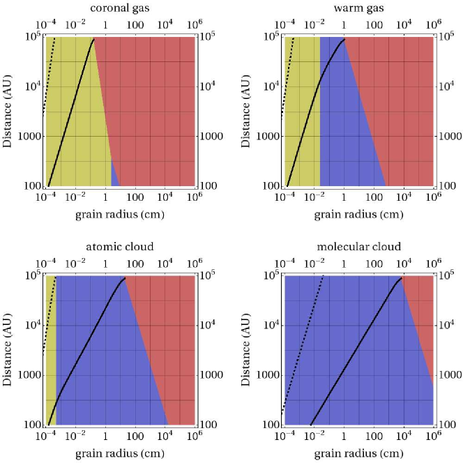
Figure 1: Map of regions in particle radius - orbital distance parameter space in which different perturbing forces dominate as shown by the different colors: yellow - electric force, blue - gas drag and Coulomb drag combined, red - galactic tide. Different panels correspond to different ISM phases as labeled on the figure. The solid line gives the particle size below which ejection occurs (see §3.3) and the dashed line gives the condition $a=d_{\text{coupl}}$ (equations [6] and [18]). We assume that the grains have a density of $1\text{ g cm}^{-3}$ and are at a potential of $1\ \text{Volt}$. The magnetic field has a strength of $5\ \mu\text{G}$, and the ISM properties are the same as those listed in Table 1.

2.4 Radiation Forces

There are several ways in which radiation affects the grain motion. Solar radiation exerts the radiation pressure force on dust particles

$$F_{\text{rad}}=\frac{L_{\odot}r_{g}^{2}}{4a^{2}c}\langle Q\rangle,$$ (25)

where $c$ is the speed of light and $\langle Q\rangle$ is a frequency-averaged radiation absorption and scattering coefficient (Burns et al. 1979), which equals 1 in the regime of geometrical optics. Because $F_{\text{rad}}$ is directed radially and scales in the same way as gravity, it simply modifies ${\bf F}_{g}$ to be ${\bf F}_{g}(1-\beta)$ where $\beta\equiv F_{\text{rad}}/F_{g}$. For particles larger than $1\ \mu\text{m}$ in size $\beta$ is small (Burns et al. 1979), and as we show later, particles smaller than $1\,\mu$m in size are ejected by the electric and total drag forces outside of the heliosphere (at $a>250$ AU). For that reason we simply disregard Solar radiation pressure in this study (if needed the contribution of the radiation pressure can be easily accounted for by redefining $M_{\odot}\to M_{\odot}(1-\beta)$ in all equations).

Poynting-Robertson drag is unimportant beyond $250\ \text{AU}$ since the decay time for a circular orbit is

$$\tau_{PR}=\frac{16\pi r_{g}\rho a^{2}c^{2}}{3L_{\odot}\langle Q\rangle}$$ (26)

$$=2.8\times 10^{4}\text{ Gyr}\,r_{g,2}\rho_{1}a_{4}^{2}\langle Q\rangle^{-1}$$

Although this is shorter than the age of the Solar System for $1\ \mu\text{m}$ grains inside of $10^{3}\ \text{AU}$, these grains are ejected from the Solar System on significantly shorter timescales by other non-gravitational forces as we demonstrate in §5.

The anisotropy of background starlight exerts a force $F_{\text{anis}}=\Delta\pi r_{g}^{2}u\langle Q\rangle$, where $u=10^{-12}$ erg cm^-3 (Draine, 2010) is the energy density of the background starlight and $\Delta=0.1$ (Weingartner & Draine, 2001) is a parameter quantifying the degree of anisotropy. We estimate that

$$\frac{F_{\text{anis}}}{F_{g}}=1.3\times 10^{-3}\,r_{g,2}^{-1}\,\rho_{1}^{-1}\,a_{4}^{2}\left(\frac{\Delta}{0.1}\right)\left(\frac{u}{10^{-12}\ \text{erg}\ \text{cm}^{-3}}\right)\langle Q\rangle,$$ (27)

and using equations (4) and (15) we find that $F_{\text{anis}}$ is sub-dominant compared to either the total drag, the electric force, or both in all ISM phases.

Finally, there is also a non-conservative drag force that arises due to the redshifting and blueshifting of the background starlight as the dust grain orbits the BSS, similar to the differential drag described in §2.2.1. However the magnitude of this force is $\sim F_{\text{anis}}\Delta^{-1}\left(v_{K}/c\right)$ and this is always much smaller than $|\Delta{\bf F}_{\rm drag}|\sim\left(v_{K}/v_{w}\right)F_{\text{drag}}$. Thus, for the problem at hand we can safely neglect any radiation forces on dust grains.

3 The Stark Problem

In the approximation that the ISM properties and $\bf{v}_{w}$ are held constant and $v_{w}\gg v_{K}$, the electric force and the velocity-independent total drag force $F_{{\rm drag},0}$ do not depend on the orbital parameters and are constant over an orbit. This reduces the problem of solving the grain dynamics to the classical Stark problem of motion in a Keplerian potential subject to an extra force ${\bf S}$ which is constant in magnitude and direction. In our case,

$${\bf S}={\bf F}_{E}+{\bf F}_{{\rm drag},0},$$ (28)

has both a component ${\bf F}_{{\rm drag},0}$ parallel to ${\bf v}_{w}$ and a component ${\bf F}_{E}$ orthogonal to ${\bf v}_{w}$. Thus, in general ${\bf S}$ is oriented arbitrarily with respect to ${\bf v}_{w}$.

The classical Stark problem in its most general setting, including the case of $S\equiv|{\bf S}|\gtrsim F_{g}$, has been previously explored analytically. It has been shown to be separable in parabolic coordinates by Landau & Lifshitz (1976) and by Banks & Leopold (1978), who studied the ionization of highly excited atoms by an electric field. Kirchgraber (1970) has shown that it is possible to solve it by using the Kustaanheimo-Stiefel (KS) transformation (Kustaanheimo & Stiefel 1965), which maps out the three-dimensional Keplerian problem into the four-dimensional harmonic oscillator problem. Unfortunately, the results of these studies are expressed in terms of integrals of Jacobian elliptic functions, the special functions inverse to the elliptic integrals, and are thus difficult to analyze. Nevertheless, we will use the existing analyses of the Stark problem in §3.3 to obtain an accurate description of the conditions under which particle ejection occurs.

In most of this study, however, we are interested in the motion of grains large enough for the Stark force, equation (28), to be considered a perturbation on top of $F_{g}$. We can quantify this condition as

$$\alpha\equiv\frac{Sa^{2}}{GM_{\odot}m_{g}}\ll 1,$$ (29)

where $a$ is the instantaneous value of the semi-major axis. In this limit, we can use standard methods of perturbation theory to investigate the dynamics of dust particles. Previously, Mignard & Henon (1984) have used osculating elements (Burns et al., 1979; Murray & Dermott, 2001) to solve the problem of a constant force perturbing a test particle orbiting a central mass which is stationary in a rotating reference frame. This problem is relevant to the study of a particle orbiting a planet subjected to radiation pressure from the Sun, and it is identical to the Stark problem if the rotation rate of the reference frame is set to zero.

We will approach the perturbative Stark problem ($\alpha\ll 1$) in two steps. First, in §3.1 we consider the simplified case of the planar Stark problem in which ${\bf S}$ lies in the plane of the particle orbit using osculating elements. This provides us with a simple qualitative picture of the secular evolution under the action of Stark force. We then adopt the orbit-averaged Hamiltonian formalism to study the more general Stark problem in which ${\bf S}$ can have any orientation with respect to the orbital plane. We also compare our results to numerical orbit integrations using an integrator described in Appendix C.

3.1 The Planar Stark Problem: perturbative approach.

In the case of the Stark force lying in the plane of the orbit, the motion is restricted to this plane, and the inclination of the orbit $i=90^{\circ}$ does not change. We choose a coordinate frame in this plane so that the $x$-axis is aligned with ${\bf S}$ and count the longitude of pericenter $\omega$ from this direction. The orbit averaged equations for the evolution of the osculating elements (Burns et al., 1979; Murray & Dermott, 2001) then become

$$\left\langle\frac{da}{dt}\right\rangle = 0,$$ (30)

$$\left\langle\frac{de}{dt}\right\rangle = -\frac{3}{2}\frac{JS}{GM_{\odot}m_{g}}\sin(\omega),$$ (31)

$$\left\langle\frac{d\omega}{dt}\right\rangle = -\frac{3}{2}\frac{JS}{GM_{\odot}m_{g}e}\cos(\omega),$$ (32)

where $J$ is the specific angular momentum and $e$ is the orbital eccentricity. Both $J$, $e$, and $\omega$ vary in time under the action of Stark force, while $a$ does not vary on average.

Figure 2: Evolution of (a) semi-major axis, (b) eccentricity, (c) longitude of pericenter, and (d) radius over a Stark period for an orbit with $T_{\text{stark}}/T_{K}=37$ ($\alpha$ = 0.018), $\Lambda=e(0)=0.75$ and $t_{0}=\omega(0)=0$. Solid lines correspond to solutions obtained from numerical integration, and dashed lines are the analytic solutions from equations (33) and (34). The eccentricity tends to unity when the angular momentum vector changes sign, and when this happens the particle can pass very close to the origin.

We can integrate equations (31) and (32) directly to obtain

$$e\cos\omega = \Lambda,$$ (33)

$$e\sin\omega = -\sqrt{1-\Lambda^{2}}\sin\left(2\pi\frac{t-t_{0}}{T_{\text{stark}}}\right),$$ (34)

where $\Lambda$ is the value of $e\cos\omega$ at time $t=0$, $t_{0}$ is the other integration constant, and

$$T_{\text{stark}}\equiv\frac{4\pi m_{g}}{3S}\sqrt{\frac{GM_{\odot}}{a}}=0.67\ \text{Myr}\,a_{4}^{3/2}\,\alpha^{-1}$$ (35)

is the timescale for the orbital elements to return to their original values (a Stark cycle), with $\alpha$ defined in equation (29). The ratio of the Stark period to an orbital period is $T_{\text{stark}}/T_{K}=(2/3)\alpha^{-1}$. Equation (33) agrees with the results of Pástor et al. (2010), and the Stark period was previously obtained by Mignard & Henon (1984).

In Figure 2 we show the evolution of the orbital elements over a timescale $T_{\text{stark}}/4$, which corresponds to $\alpha=0.018$. The agreement between the analytical theory (equations [33] and [34]) and numerical results is good. Note that in accordance with equation (30), the semi-major axis of the orbit stays constant because the constant perturbing force does no work over a closed orbit. However, on a time scale $T_{K}$, $a$ still experiences small oscillations with amplitude

$$\frac{\Delta a}{a}\sim 4\alpha,$$ (36)

which are due to the work done by the Stark force in the course of orbital motion.

The eccentricity of the orbit varies through the Stark cycle from $\Lambda$ to $1$, thus allowing very close approaches of particles to the Sun. As we will see in the next section, such high values of $e$ are a peculiarity of the planar Stark problem, but the periodic variations of $e$ and $\omega$ are generic.

3.2 The General Stark Problem: perturbative approach

Following the procedure outlined in Heisler & Tremaine (1986), we treat the general Stark problem of an arbitrarily oriented Stark force ${\bf S}$ by orbit-averaging the particle Hamiltonian and determining the integrals of motion. This procedure is different from the approach of Pástor et al. (2010) and Mignard & Henon (1984) who used orbit averaged equations for the evolution of the osculating elements (Burns et al., 1979; Murray & Dermott, 2001) to treat the general Stark problem.

If we align the $z$-axis with ${\bf S}$, the Hamiltonian per unit mass becomes

$$H=\frac{v^{2}}{2}-\frac{GM_{\odot}}{r}-\frac{S}{m_{g}}z.$$ (37)

Using the relations $z=r\sin i\sin(f+\omega)$ and $r=a(1-e^{2})/(1+e\cos f)$, where $f$ is the true anomaly (varying on an orbital timescale), we can rewrite this expression as

$$H=-\frac{GM_{\odot}}{2a}+\frac{Sa(1-e^{2})\sin(f+\omega)\sin i}{m_{g}(1+e\cos f)}.$$ (38)

When $\alpha\ll 1$ the orbital elements vary on a timescale $T_{\text{stark}}$, which is much longer than $T_{K}$. Averaging the Hamiltonian over a closed Keplerian orbit we obtain

$$H_{\rm av}=-\frac{GM_{\odot}}{2a}-\frac{3S}{2m_{g}}a\,e\,\sin i\,\sin\omega.$$ (39)

By introducing the Delaunay angle-action variables (Binney & Tremaine 2008)

$$l L=\sqrt{GM_{\odot}a}$$ , (40)

$$\omega J=\sqrt{GM_{\odot}a(1-e^{2})}$$ , (41)

$$\Omega J_{z}=J\cos i$$ , (42)

($l$ is the mean anomaly, $\Omega$ is the longitude of ascending node) we rewrite the time-averaged Hamiltonian as

$$H_{\text{av}}=-\frac{(GM_{\odot})^{2}}{2L^{2}}-\frac{3}{2}\frac{SL^{2}}{GM_{\odot}m_{g}}\sqrt{1-\frac{J^{2}}{L^{2}}}\sqrt{1-\frac{J_{z}^{2}}{J^{2}}}\sin\omega.$$ (43)

Because the Delaunay variables are canonically conjugate and the Hamiltonian is independent of $l$, $\Omega$, and $t$, we immediately see that $L$, $J_{z}$, and $H_{\text{av}}$ must be conserved, implying that the semi-major axis, the $z$-component of the angular momentum, and total energy do not change on average. The total angular momentum $J$ is not conserved, so that $e$, $i$, $\omega$ and $\Omega$ must vary under the action of Stark force.

Introducing dimensionless variables

$$K=\frac{J}{L},~{}~{}~{}~{}K_{z}=\frac{|J_{z}|}{L},$$ (44)

we find from equation (43) that

$$(\Delta\tilde{H})^{2}=(1-K^{2})\left(1-\frac{K_{z}^{2}}{K^{2}}\right)\sin^{2}\omega,$$ (45)

is an integral of motion which we will use from now on instead of $H_{\rm av}$. It is easy to see that $0\leq\Delta\tilde{H}\leq 1-K_{z}$.

Conservation of $\Delta\tilde{H}$ and $K_{z}$ allows us to directly relate $K$ to $\omega$. For a given value of $K_{z}$ in $K-\omega$ space, the particle is confined to move on contours of constant $\Delta\tilde{H}$. We have plotted the contours for $K_{z}=0.5$ in Figure 3 along with the numerically integrated particle trajectory in these coordinates. This figure clearly shows the existence of a stationary solution when $\Delta\tilde{H}$ takes its maximum value of $1-K_{z}$ with both $K=\sqrt{K_{z}}$ and $\omega=\pi/2$ constant in time. The three-dimensional trajectory of this orbit is shown in Figure 3, and it is obvious that $\Omega$ is the only orbital element of the stationary orbit that varies with time (equation [51]).

We now determine the explicit time dependence of $e$, $i$, $\omega$ and $\Omega$ in the general case for arbitrary $J_{z},L,\text{ and }\Delta\tilde{H}$. The evolution of $\omega$ is governed by the equation

$$\frac{d\omega}{dt}=\frac{\partial H_{\text{av}}}{\partial J}=-\frac{3}{2}\frac{SL}{GM_{\odot}m_{g}}\frac{K_{z}^{2}-K^{4}}{K^{2}\sqrt{(1-K^{2})(K^{2}-K_{z}^{2})}}\sin\omega,$$ (46)

where $H_{\text{av}}$ is the Hamiltonian in equation (43)). Using equation (45) to express $\sin\omega$ and $d\omega/dK$ as functions of $K$ we derive the following equation for the evolution of $K$:

$$\frac{dK}{dt}=\frac{3}{2}\frac{SL}{GM_{\odot}m_{g}}\frac{\sqrt{(K_{\text{max}}^{2}-K^{2})(K^{2}-K_{\text{min}}^{2})}}{K},$$ (47)

where

$$K^{2}_{\{^{\text{max}}_{\text{min}}\}}=\frac{1+K_{z}^{2}-(\Delta\tilde{H})^{2}}{2}\pm\left[\left(\frac{1+K_{z}^{2}-(\Delta\tilde{H})^{2}}{2}\right)^{2}-K_{z}^{2}\right]^{1/2}$$ (48)

are the maximum and minimum possible values of $K^{2}$ for given $K_{z}$ and $\Delta\tilde{H}$. Integrating equation (47) one finds

$$K^{2}(t)=\frac{K_{\text{min}}^{2}+K_{\text{max}}^{2}}{2}+\frac{K_{\text{max}}^{2}-K_{\text{min}}^{2}}{2}\sin\left(4\pi\frac{t-t_{0}}{T_{\text{stark}}}\right),$$ (49)

where $t_{0}$ is the integration constant. It immediately follows from this solution that the timescale for the orbit to go once around a contour in $K-\omega$ space (Figure 3) is $T_{\text{stark}}/2$ independent of $K_{z}$ and $\Delta\tilde{H}$.

Since $e^{2}(t)=1-K^{2}(t)$ and $\cos i=K_{z}/K(t)$ (equation [44]), the solution, equation (49), immediately gives us the time dependence of $e$ and $i$. Also, equation (45) connecting $\omega$ and $K$ enables us to determine explicitly the evolution of $\omega(t)$.

Finally, to determine the evolution of $\Omega$, we use the equation

$$\frac{d\Omega}{dt}=\frac{\partial H_{\rm av}}{\partial J_{z}}=\frac{3}{2}\frac{SL}{GM_{\odot}m_{g}}\frac{\sqrt{1-K^{2}}}{\sqrt{K^{2}-K_{z}^{2}}}\frac{K_{z}}{K}\sin\omega.$$ (50)

Equation (47) allows us to convert this expression into an equation for $\Omega(K)$ with the solution

$$\Omega(K)=\arctan\left(\sqrt{\frac{(K^{2}-K_{\text{min}}^{2})(K_{\text{max}}^{2}-K_{z}^{2})}{(K_{\text{max}}^{2}-K^{2})(K_{\text{min}}^{2}-K_{z}^{2})}}\right).$$ (51)

Since the argument of arctangent in the numerator of equation (51) vanishes at $K=K_{\text{min}}$ and the denominator equals zero for $K=K_{\text{max}}$, we have $\Omega(K_{\text{max}})-\Omega(K_{\text{min}})=\pi/2$. Because $K$ goes from $K_{\text{min}}$ to $K_{\text{max}}$ on a timescale of $T_{\text{stark}}/4$, $\Omega$ goes from 0 to $2\pi$ on a timescale of $T_{\text{stark}}$. Thus, all of the orbital elements return to their original values after a time $T_{\text{stark}}$ in the general case just as in the planar case. The stationary solution has $\Omega$ linearly growing in time, which is most easily seen directly from equation (50) but can also be derived by taking the limit $\Delta\tilde{H}\to 1-K_{z}$, $K\to\sqrt{K_{z}}$ in equation (51).

These results allow us to put constraints on the possible values of eccentricity and inclination that an orbit attains during its Stark cycle. The minimum and maximum values of $K$ are $K_{\text{min}}$ and $K_{\text{max}}$, and $\cos i$ oscillates between $K_{z}/K_{\text{max}}$ and $K_{z}/K_{\text{min}}$, while the eccentricity $e$ varies between $\left(1-K_{\text{max}}^{2}\right)^{1/2}$ and $\left(1-K_{\text{min}}^{2}\right)^{1/2}$. Since $K_{z}\leq K_{\text{min}}$, the eccentricity only evolves to unity if the Stark vector is in the plane of the orbit ($K_{z}=0$).

Mignard & Henon (1984) have previously found implicit formulas for the time dependence of the orbital elements. Their results also apply to a rotating reference frame, but our formulae are more straightforward to use in the case of the Stark problem, since they give a simple, explicit prescription for the evolution of the orbital elements.

Figure 4 compares the analytic expressions for $K^{2}(t)=1-e^{2}(t)$, $i(t)$, $\omega(t)$, and $\Omega(t)$ with numerical integrations. Good agreement between the two approaches can be seen if one disregards the small-amplitude oscillations of orbital elements on a time scale $T_{K}$ which are not captured by our orbit-averaged theory.

We have assumed in §§3.1 and 3.2 that the Stark vector is constant, but in reality it can vary in both magnitude and direction due to effects such as a changing relative velocity between the Solar System and the ISM, a variation in the particle’s charge as a function of distance from the Sun, small scale magnetic turbulence in the ISM, etc. We study these effects in Appendix A and conclude that most likely they add details to, but do not significantly change the general picture presented in §§3.1 and 3.2.

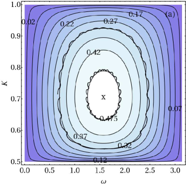
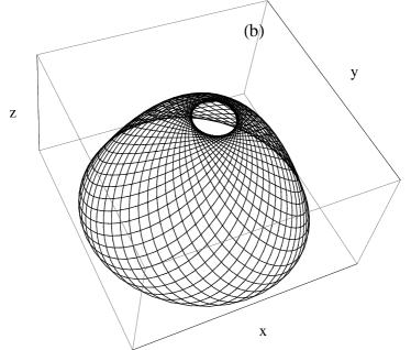
Figure 3: (a) Contours of constant $\Delta\tilde{H}$ (labeled by the value of $\Delta\tilde{H}$) for $K_{z}=0.5$ with numerically integrated orbits over-plotted (both orbits have $\alpha=0.02)$. The orbits do not exactly follow a contour due to our orbit-averaging of the Hamiltonian. (b) Trajectory of the stationary orbit ($\alpha=0.02$, $K_{z}=0.5$) for which $a$, $e$, $i$, and $\omega$ all remain constant, while $\Omega$ increases at a constant rate. The stationary orbit is marked by a cross in panel (a).

Figure 4: Plots of (a) $K^{2}(t)$, (b) $\Omega(t)$, (c) $i(t)$, and (d) $\omega(t)$ for an orbit with $K_{z}=0.6$, $\Delta\tilde{H}=0.34$, and $\alpha=0.04$. Dashed lines show results from orbit-averaged theory (equations [46] - [51]), and the solid lines show results from numerical integrations.

3.3 The general Stark problem: particle ejection

When $\alpha\sim 1$ our perturbative approach used in §3.1-§3.2 breaks down. In fact, for $\alpha\gtrsim 1$ one expects the particle to become unbound since the Stark force becomes larger than $F_{g}$. We now perform a detailed treatment of particle ejection with the goal of determining the value of $\alpha$ that yields ejection for different initial conditions.

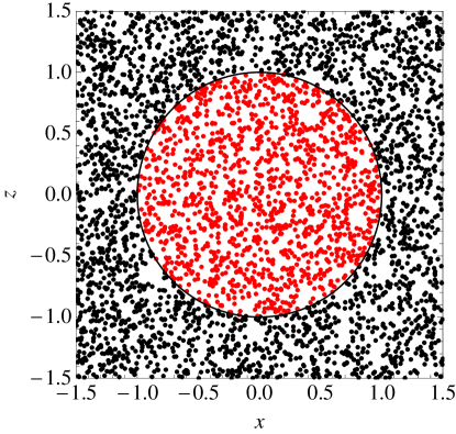
Figure 5: Illustration of the ejection criterion for particles initialized at rest, showing the outcome of the numerical integration of an orbit (black - ejection, red - orbits bound after an integration time of 10 $T_{K}$). The Stark force is directed along the z-axis and because of rotational symmetry we only need to consider particles initialized in the x-z plane. The black circle shows the radius of the sphere beyond which orbits are unbound as given by the ejection criterion (equation [52]), and the units on the axes are scaled so that the sphere has a radius of one. The numerical integrations agree with equation (52), since only those particles initialized outside of a radius of one are ejected within 10 $T_{K}$ (most unbound particles are ejected within 1 $T_{K}$, so virtually all unbound particles should be ejected after 10 $T_{K}$.).

Kirchgraber (1971), Dankowicz (1994), and Banks & Leopold (1978) have previously made attempts to study ejection in the Stark problem but their results are not easy to interpret. In Appendix B we show that using the approach of Kirchgraber (1971) it is still possible to derive a set of simple analytical criteria for testing whether a particle with a given initial position ${\bf r}^{0}$ and velocity ${\bf v}^{0}$ is bound or unbound (equations [B2]-[B8]). In finding these criteria we did not use the rather complicated solutions for particle motion obtained in Kirchgraber (1971), but instead resorted to general energetic arguments applied to the particle Hamiltonian expressed in Kustaanheimo-Stiefel variables (Kustaanheimo & Stiefel 1965).

The Stark force introduces a preferred direction into the otherwise isotropic Keplerian problem. Thus, one expects that in general the ejection criterion would depend not only on the initial particle distance from the BSS but also on the direction of ${\bf r}^{0}$ and on ${\bf v}^{0}$. Quite interestingly, we find in Appendix B that in the case of dust grains starting at rest with respect to the BSS (${\bf v}^{0}=0$) the ejection criterion is independent of the direction of ${\bf r}^{0}$ and simply states that all particles with

$$\alpha>0.25,~{}~{}~{}~{}~{}|{\bf v}^{0}|=0,$$ (52)

are going to be ejected from the system. Figure 5 illustrates this simple ejection criterion computationally: orbits of a number of particles with randomly chosen ${\bf r}^{0}$ and $|{\bf v}^{0}|=0$ have been integrated for ten orbital timescales each to determine whether they are bound or not; the condition (52) clearly works quite well.

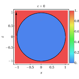
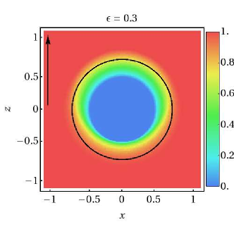
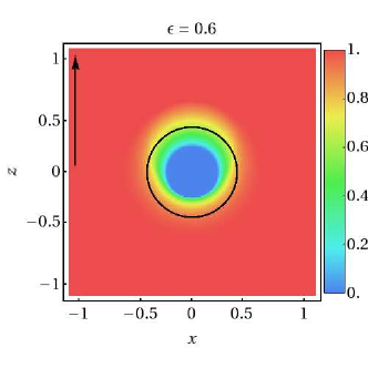
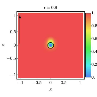
Figure 6: Ejection in the case of non-zero initial velocity. The Stark vector points in the $+z$ direction, as indicated by the arrows, so the problem is rotationally symmetric about the z-axis, and we confine ourselves to the x-z plane. Each panel shows the fraction of ejected particles as a function of starting position for a given value of $\epsilon$ (defined in the text). Red corresponds to all particles initialized at a given location being ejected and blue corresponds to all particles being bound after 10 $T_{K}$. The scale of the $x$ and $z$ axes is the same in each plot and is normalized by the value of the semi-major axis at which $\alpha=0.25$ in the zero velocity case ($\epsilon=0$). The black circle shows the $\alpha=0.25$ contour for the value of $\epsilon$ with which particles are initialized (it contracts inwards with increasing $\epsilon$ because of the relation $a^{0}=r^{0}/2(1-\epsilon)$).

To study the case of a nonzero initial velocity, we performed Monte Carlo simulations where we initialized particles at a given radius to have a random orientation of ${\bf v}^{0}$ and a kinetic energy which is a fixed fraction $\epsilon$ of their gravitational potential energy: $\left(v^{0}\right)^{2}/2=\epsilon GM_{\odot}/r^{0}$. The initial semi-major axis $a^{0}$ can then be expressed in terms of the initial radius as $a^{0}=r^{0}/2(1-\epsilon)$, which allows the calculation of $\alpha$ in each case. The case of zero initial velocity corresponds to $\epsilon=0$. In all non-zero initial velocity cases simulated here we found the general analytical ejection criteria (B2)-(B8) to correctly predict whether particles are bound to the Solar System.

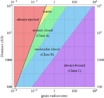
Figure 7: Map of the ejection regimes in particle radius - orbital distance space. In the purple region, particles are bound regardless of the ISM phase (Class C particles, §5.3). In the adjacent light blue region, particles will be ejected when passing through a molecular cloud, but will be bound in all other phases (Class B particles, §5.2). In the green region, particles will be ejected in atomic clouds and molecular clouds, but will be bound otherwise (Class A particles, §5.1). In the yellow region particles are only bound in the coronal phase (also Class A particles, §5.1). In the red region, particles are unbound in all ISM phases, and the boundary of this region is given by equation (5), which is shown as a black line on the plot.

Figure 6 shows the effect of varying $\epsilon$ on the value of $\alpha$ required for ejection. In the case of $|{\bf v}^{0}|\neq 0$, each initial particle position is characterized by some probability of ejection since whether a body is ejected or not depends on the orientation of ${\bf v}^{0}$, and we display these probabilities with color maps. Most notably, Figure 6 shows that for $\epsilon>0$ there exists an outer boundary beyond which all particles are ejected regardless of their initial velocity, an inner boundary inside of which all orbits are bound for $\epsilon<1$, and a region in between in which orbits can be bound or unbound depending on the orientation of ${\bf v}^{0}$. As ${\bf v}^{0}$ increases and $\epsilon$ becomes larger, the inner and outer ejection boundaries become more elongated along the direction of ${\bf S}$, and ejection can occur for certain orbits even if $\alpha<0.25$, whereas some orbits can remain bound even if $\alpha>0.25$. However, even for $\epsilon$ as high as $0.9$ the simple ejection criterion (equation [52]) still provides a good estimate of the radius at which particles become unbound to within a factor of two.

In Figure 7 we use the ejection criterion from equation (52) to determine whether particles are bound or unbound at different separations from the BSS in different ISM phases. It clearly demonstrates that independent of the inflowing ISM phase, particles as large as $r_{g}=150\,\mu$m should be ejected by the electromagnetic force at $a=10^{4}$ AU, while at $a=10^{3}$ AU only particles with $r_{g}\lesssim 15\,\mu$m are unbound (equation [5]). Bigger grains can also be removed in passages through the denser phases of the ISM. In particular, passages through molecular clouds would eject bodies as large as $1$ m in size at $10^{4}$ AU due to the total drag force, in agreement with Stern (1990).

Very small particles for which $\alpha\gg 1$ should be rapidly coupled to the ISM flow by the non-gravitational forces. We introduce the coupling particle size $r_{g,{\rm coupl}}$ as the size for which the coupling distance is equal to the initial particle semi-major axis, i.e. $d_{\rm coupl}(r_{g,{\rm coupl}})=a$. Particles with $r_{g}\lesssim r_{g,\text{coupl}}$ rapidly attain a velocity $\sim v_{w}$ in the solar frame. This makes it necessary to consider the Stark force as a function of velocity and take the magnetic force into consideration, since the relation $v\sim v_{K}\ll v_{w}$ is no longer valid. The dependence of $r_{g,{\rm coupl}}$ on $a$ is shown in Figure 1 by a dashed line. It is clear that efficient coupling to the ISM on scales of order the initial size of the system is possible only for particles with $r_{g}$ considerably smaller than the size at which ejection occurs. Particles with $r_{g}\gtrsim r_{g,{\rm coupl}}$ passing close to the Inner Solar System should have speeds considerably different from (smaller than) $v_{w}$.

4 Orbital Decay via the Differential Drag

We now consider the effect of the differential drag force $\Delta{\bf F}_{\text{drag}}$ on the motion of dust particles. $\Delta{\bf F}_{\text{drag}}$ explicitly depends on the Keplerian velocity of the grain, and plugging the expression for $\Delta{\bf F}_{\text{drag}}$ from equation (19) into the equations for the evolution of the osculating elements (Burns et al., 1979; Murray & Dermott, 2001), one obtains the following equation for the orbit-averaged rate of change of the semi-major axis

$$\left\langle\frac{da}{dt}\right\rangle=-\frac{2a}{m_{g}v_{w}}\left[F(v_{w})(1-\beta)+\frac{dF}{dv}\Big{|}_{v=v_{w}}v_{w}\beta\right],$$ (53)

where we have defined

$$\beta\equiv e^{-2}\left[\left(1-\sqrt{1-e^{2}}\right)\left(\frac{{\bf v}_{w}\cdot\hat{\bf a}}{v_{w}}\right)^{2}+\left(e^{2}-1+\sqrt{1-e^{2}}\right)\left(\frac{{\bf v}_{w}\cdot\hat{\bf b}}{v_{w}}\right)^{2}\right],$$ (54)

and ${\bf\hat{a}}$, ${\bf\hat{b}}$, and ${\bf\hat{c}}$ are orthonormal unit vectors with ${\bf\hat{a}}$ pointing towards the pericenter, ${\bf\hat{c}}$ aligned with the particle’s angular momentum vector, and ${\bf\hat{b}}={\bf\hat{c}}\times{\bf\hat{a}}$ (Burns et al., 1979). Equation (53) agrees with the results of Pástor et al. 2010 who obtained it for the special case of a drag force that depends quadratically on the velocity.

The parameter $\beta$ has the property that $0\leq\beta\leq 1$ for any $e<1$. Although $\beta$ varies on timescales of order $T_{\text{stark}}$ because of the secular changes in eccentricity and orientation of the orbit, we can average the right-hand side of equation (53) over a Stark orbit to obtain

$$\left\langle a(t)\right\rangle = a_{0}e^{-\gamma t}$$ (55)

$$\gamma \equiv \frac{2}{m_{g}v_{w}}\left[F(v_{w})(1-\langle\beta\rangle_{S})+\frac{dF}{dv}\Big{|}_{v=v_{w}}v_{w}\langle\beta\rangle_{S}\right],$$ (56)

where angle brackets with a subscript $S$ denote time-averaging over a Stark orbit, angle brackets without a subscript denote time-averaging over a Keplerian orbit, and $a_{0}$ is the initial value of the semi-major axis. The validity of averaging over a Stark orbit in equation (55) hinges upon $\gamma^{-1}\gg T_{\text{stark}}$, since this is the condition for the orbit to be only slightly modified by the differential drag over a timescale $T_{\text{stark}}$. This condition is satisfied in practice, since according to equations (35) and (56)

$$\gamma T_{\text{stark}}\sim\frac{v_{K}F_{\text{drag}}}{v_{w}S}\ll 1,$$ (57)

where $S\gtrsim F_{\text{drag}}$ ($S>F_{\text{drag}}$ if, for example, the electric force dominates the total drag force). Thus, as long as $v_{K}/v_{w}\ll 1$, the semi-major axis evolves exponentially with an instantaneous decay constant given by $\gamma$.

An immediate consequence of equation (56) is that the semi-major axis can either grow or decay in time depending on the value of $\beta$ and the sign of $dF/dv$. For gas drag, $dF/dv>0$ for any $v$, so $\gamma>0$, and the orbit always decays with time. On the other hand, for pure Coulomb drag $dF/dv<0$ if the Mach number of the ISM flow with respect to the sound speed of the ionized component $s\gtrsim 0.968$ (equations [9]-[14]). Thus, depending on the value of $\beta$, the semi-major axis can either grow or decay with time.

An interesting question is whether differential drag can cause the expansion of particle orbits under realistic ISM conditions. According to equation (56) this amounts to a calculation of $dF/dv|_{v=v_{w}}$ where $F$ is the magnitude of the force due to both gas and Coulomb drag combined under actual ISM conditions. The results of such a calculations are presented in Figure 8 and clearly show that for any grain size in any of the ISM phases $dF/dv|_{v=v_{w}}>0$, meaning that a particle’s semi-major axis can only decay ($\gamma>0$) under the action of the differential drag force.

Figure 8: Plot of $d\ln F/d\ln v|_{v=v_{w}}$ as a function of grain size for various ISM phases, where $F$ is the sum of Coulomb and gas drag forces. Because $d\ln F/d\ln v|_{v=v_{w}}>0$ over the whole range of grain sizes for each phase of the ISM, the differential drag always causes the semi-major axes of particle orbits to decay, see equation (53).

5 Application to Grains in the Outer Solar System

Having explored the forces that affect the dynamics of dust grains in the OSS, we are now in a position to describe their long-term evolution after they have been created in collisions of larger objects (e.g. comets). Our discussion will predominantly focus on two important questions. First, what is the survival time $T_{s}$ of a dust particle of a given size located at a given separation from the BSS against ejection by the ISM flow. Second, how does the semi-major axis of a particle change as a result of differential drag during its lifetime in the OSS?

In addressing these questions we must realize that through its 4.5 Gyr history, the Solar System has sampled different phases of the ISM, which must have subjected dust grains in the OSS to broadly varying ambient conditions. As a result, grains which are only weakly affected by the ISM flow when the Solar System passes through one phase (e.g. the coronal gas) may become fully coupled to this flow in another phase (e.g. a molecular cloud), see Figure 1. Therefore there are several possible classes into which dust grains can be separated from the point of view of their long-term dynamics:

• Class A covers particles which can survive ejection in the warm and coronal phases of the ISM, but which will be ejected in a passage through an atomic or molecular cloud.

• Class B involves particles which are large enough to survive ejection in atomic clouds, but which would be ejected in passages through molecular clouds.

• Class C covers particles which are large enough to survive ejection in a molecular cloud. Thus these particles can survive ejection in any phase of the ISM.

The assignment of a given dust grain to a particular class depends not only on the particle size but also on the particle distance from the BSS. Figure 7 shows the map of different Classes in the $r_{g}-a$ space. Note that particles satisfying the condition $r_{g}<r_{g,\text{min}}$ with $r_{g,\text{min}}$ defined in equation (5) do not exhibit long-term dynamics on the OSS as they get rapidly ejected by the electric force even in the coronal phase of the ISM. For that reason we do not introduce a separate class for these small grains.

5.1 Class A

Stern (1990) quotes $40$ Myr for the average time between passages through atomic clouds. This is roughly survival time, $T_{s}$, of Class A particles since these are ejected in passages through atomic or molecular clouds, but passages through molecular clouds happen on much longer, $\sim 400\ \text{Myr}$ (Stern, 1990), timescales.

We now study the decay in semi-major axis caused by the differential drag in the coronal and warm phases of the ISM in between ejection events. We consider particles at $3000$ AU with $\rho=1$ g cm^-3 and $\alpha=0.05$, which corresponds to a grain radius $r_{g}\approx 100\ \mu\text{m}$ for both the coronal and warm phases. The reason the grain radii are the same in different phases is because the electric force is the dominant perturbation in both cases, and we are assuming the particles are charged to the same potential of $1$ V. Our choice of $\alpha$ is close to the threshold indicated in the ejection criterion (52) and is motivated by the fact that differential drag is most important for the smallest particles.

Equation (55) predicts roughly exponential decay of the particle orbit on some characteristic time scale $t_{\text{decay}}=\gamma^{-1}$. To evaluate upper and lower limits for $t_{\text{decay}}$, we calculate $\gamma^{-1}$ in equation (56) for $\beta=0$ and $\beta=1$. We can immediately rule out differential drag playing an important role in the coronal phase, since $2.8\ \text{Gyr}<t_{\text{decay}}<3.0\ \text{Gyr}$ there, which is much longer than the $40$ Myr interval between ejection events. On the other hand, a similar calculation for the warm phase yields $27\ \text{Myr}<t_{A,\text{decay}}<38\ \text{Myr}$. Since this is smaller than $T_{s}\sim 40\ \text{Myr}$, the semi-major axes of some Class A particles can decay by a factor of a few between ejection events.

To verify our estimate for $t_{\text{decay}}$ in the warm phase, we perform Monte Carlo simulations of dust grain orbital evolution. We initialize particles to have a semi-major axis of $3000\ \text{AU}$, corresponding to the inner edge of the Oort Cloud where most of the dust should be concentrated. Without good knowledge of what the distribution of the other orbital elements should be, we choose the eccentricities uniformly on the interval $(0,0.99)$, and randomly orient the orbit in space. The perturbations included in the simulation on top of the gravitational attraction to the BSS are the electric force, gas drag, and Coulomb drag; other perturbations forces are unimportant for particles of this size at this semimajor axis.

We simulate $10^{4}$ orbits for $40$ Myr assuming particle parameters adopted for Class A (see above). For each run we compute the average $\gamma$ over the length of the simulation by finding a best exponential fit to the dependence of the semi-major axis on time. A typical example for the evolution of the semi-major axis of a particle having $\alpha=0.05$, but with a starting semi-major axis of $10^{4}\ \text{AU}$ rather than $3000\ \text{AU}$ is shown in Figure 9a. The reason for choosing $10^{4}\ \text{AU}$ for the starting semi-major axis is to highlight the rapid oscillations happening on an orbital timescale, the long oscillations occurring on a Stark period timescale, and the steady decay due to differential drag. The resulting distribution of decay times, $t_{\text{decay}}=\gamma^{-1}$, is plotted in Figure 10a. We calculate from this distribution that the mean decay time for Class A grains is $\langle t_{\text{decay}}\rangle=30.4$ Myr with a standard deviation of $1.1$ Myr. This agrees nicely with the analytical limits given above.

Furthermore, we see from equation (56) that the limits on $t_{\text{decay}}$ do not depend on the semimajor axis. Thus, as long as a grain is not eroded or destroyed in a collision, and the limits on $t_{\text{decay}}$ are tight, $\gamma$ will be approximately constant for a grain of a given size as it decays. Of course, smaller and smaller particles become bound as the semimajor axis decreases, so for $\alpha=0.05$ ($r_{g}\approx 10\ \mu\text{m}$) at $300$ AU in the warm phase, the limits on $t_{\text{decay}}$ are a mere $2.6\ \text{Myr}<t_{\text{decay}}<4.3\ \text{Myr}$, whereas at $10^{4}$ AU for $\alpha=0.05$ ($r_{g}\approx 500\ \mu\text{m}$) they are $150\ \text{Myr}<t_{\text{decay}}<180\ \text{Myr}$, substantially longer than the timescale between passages through atomic clouds.

The orbital decay of Class A particles should lead to their preferential concentration at small radii, which may promote fragmentation of these grains in mutual collisions and the creation of even smaller debris particles closer to the Sun. The implications of this effect are discussed in more detail in §6.

Figure 9: (a) The decay of a particle with an initial semi-major axis of $10^{4}\ \text{AU}$ and $\alpha=0.05$ over $40\ \text{Myr}$ in the warm phase. The rapid oscillations are on an orbital timescale and the long oscillations are on a Stark period timescale. The dashed line is the best fit exponential to the decay. (b) The decay of a Class B particle. The jumps in semi-major axis occur when the particle is passing through an atomic cloud. The dashed line is again the best fit exponential to the decay. (c) Zoomed in view of one of the passages through an atomic cloud from panel (b).

5.2 Class B

Class B comprises particles which are large enough to survive ejection in atomic clouds, but not in molecular clouds. The time between the Solar System’s passages through molecular clouds is about $400\ \text{Myr}$ (Stern, 1990), so this is the survival time for Class B dust grains.

We take the parameters of a typical Class B particle to be $\rho=1\text{ g cm}^{-3}$ and $r_{g}\approx 0.1\ \text{cm}$, since such a particle would have $\alpha=0.05$ in an atomic cloud at $a=3000\ \text{AU}$. Prior to ejection in a molecular cloud, the particle will spend a fraction $f_{\text{atomic}}$ of its lifetime in atomic clouds, where $f_{\text{atomic}}\sim 0.01$ is the filling fraction of these clouds, and a fraction $1-f_{\text{atomic}}$ of its lifetime in the warm and coronal phases combined, see Table 1. For simplicity, we assume that the particle spends its time in either the warm phase or an atomic cloud before it is ejected. Then, the characteristic decay time is $t_{\text{decay}}=[(\gamma_{\text{WISM}}(1-f_{\text{atomic}})+\gamma_{\text{atomic}}f_{\text{atomic}})]^{-1}$, where $\gamma_{\text{WISM}}$ is the value of the decay constant $\gamma$ in the warm phase and $\gamma_{\text{atomic}}$ is $\gamma$ in atomic clouds. Even though $f_{\text{atomic}}\ll 1$ the contribution to the decay from atomic clouds is still important since the total drag in them is much larger than in the more dilute phases of the ISM. Setting as in §5.1 $\beta=0$ and $\beta=1$ in equation (56) to get upper and lower bounds on the decay time we have $205\ \text{Myr}<t_{B,\text{decay}}<255\ \text{Myr}$. This is shorter than the $T_{s}=400$ Myr time between passages through a molecular cloud, so the orbits of these particles can also decay appreciably before ejection occurs.

We checked our analytical estimates by simulating $10^{4}$ particle orbits for $400\ \text{Myr}$ initialized in the same way as in §5.1 (with Class B particle parameters adopted here). We simulate the effect of passages through atomic clouds as stochastic events that happen on average every $50$ Myr, so that there are on average 8 passages through atomic clouds per simulation, and the total time spent in atomic clouds per simulation is on average $4$ Myr, consistent with $f_{v}=0.01$. A typical example of the orbital evolution of a Class B dust particle along with the best exponential fit is shown in Figures 9b,c.

The distribution of decay times $\gamma^{-1}$ is shown in Figure 10b. The mean decay time for this simulation is $\langle t_{\text{decay}}\rangle=232$ Myr with a standard deviation of $24$ Myr in agreement with analytical estimates. Note that the distributions of $t_{\text{decay}}$ for Class A and Class B particles look quite different. This is because for Class B there is an additional source of variance that is not present for Class A: we model the passages through atomic clouds as stochastic events, and thus, although there are on average 8 cloud passages per simulation, the number and timing of passages in any given simulation do not have to be the same. As a result, the distribution of $t_{\text{decay}}$ for Class B particles is closer to Gaussian.

We also give limits on $t_{\text{decay}}$ for Class B particles with starting semimajor axes at 300 AU and $10^{4}$ AU. For $\alpha=0.05$ ($r_{g}=20\ \mu\text{m}$) in an atomic cloud at $300$ AU the decay time is $2.8\ \text{Myr}<t_{B,\text{decay}}<5.2\ \text{Myr}$, so transport is extremely important for these particles if they are not destroyed on even smaller timescales (e.g. by collisions). On the other hand at $10^{4}$ AU and $\alpha=0.05$ ($r_{g}=1\ \text{cm}$), the decay time is $2.2\ \text{Gyr}<t_{B,\text{decay}}<2.6\ \text{Gyr}$ so transport is insignificant, since passages through molecular clouds happen on shorter timescales.

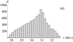
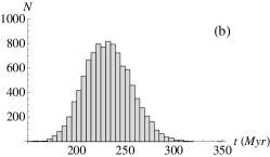
Figure 10: (a) The distribution of decay times obtained from simulations for Class A particles (§5.1). Particles with $\rho=1\text{ g cm}^{-3}$ and $r_{g}\approx 100\ \mu\text{m}$ were initialized with a semi-major axis of $3000\ \text{AU}$ and an eccentricity uniformly selected on the interval (0,0.99). The simulation was run for $40\ \text{Myr}$, and a decay constant was obtained by fitting an exponential to the $a(t)$ dependence as shown in Figure 9. (b) The distribution of decay times for particles with $\rho=1\text{ g cm}^{-3}$ and $r_{g}\approx 0.1\text{ cm}$ (Class B parameters, see §5.2). Eccentricities and semi-major axes are initialized in the same way as in (a), but the integration is now for 400 Myr and we have included the effects of passages through atomic clouds (see §5.2 for more details).

5.3 Class C

Class C particles survive passages through molecular clouds which implies that they have $T_{s}=4.5$ Gyr, i.e. the age of the Solar System. At $3000\ \text{AU}$ a particle with $\rho=1\text{ g cm}^{-3}$ and $r_{g}\approx 30\ \text{cm}$ has $\alpha=0.05$ in a molecular cloud so we take these to be the parameters of a Class C particle. Using values for the filling fractions from Table 1 and the formula

$$t_{C,\text{decay}}=\left(\displaystyle\sum_{i}\gamma_{i}f_{i}\right)^{-1},$$ (58)

where the sum runs over the different phases of the ISM, and $\gamma_{i}$ and $f_{i}$ are the corresponding orbital decay constants and filling factors, the decay time is $33\ \text{Gyr}<t_{\text{decay}}<56\ \text{Gyr}$, which is considerably longer than $T_{s}$. A particle with $\alpha=0.05$ in a molecular cloud would need to have a semimajor axis of $1000$ AU for the decay time to equal the age of the solar system (the size of such a particle would be $r_{g}\approx 3\ \text{cm}$). Thus, beyond $1000$ AU, differential drag is unimportant for Class C particles, and they should remain at essentially the same semi-major axis at which they were created.

5.4 Comparison with previous work

Stern (1990) has previously estimated the perturbing force on particles in the Oort Cloud. However, he only considered gas dynamical drag and neglected both the Coulomb drag and the electric force. Moreover, his estimates for the gas drag rely on the assumption that $v_{w}$ is much larger than the thermal velocity of the species in the wind, i.e. $s\gg 1$. From Table 1 we see that this assumption is questionable for the warm phase and incorrect for the coronal phase.

Stern (1990) has also considered the importance of a passing shock from a nearby supernova for ejecting particles and has found that a supernova at 40 pc can eject particles of radius $\sim 100\ \mu\text{m}$. Assuming a local supernova rate of 0.02 yr^-1, the average time between supernova explosions within 40 pc is $\sim 40\ \text{Myr}$. This is similar to the timescale for passages through atomic clouds, and because a typical class A particle has a radius of $r_{g}\sim 100\ \mu\text{m}$, the effect of supernova explosions is simply to reduce the average lifetime of the smaller Class A particles by about a factor of two.

Finally, Stern (1990) has pointed out that Oort Cloud objects should be eroded by high velocity impacts with interstellar grains. This is most relevant for Class A grains since they will be eroded within $40\ \text{Myr}$, according to Stern’s estimates. Thus it may be possible that these particles are eroded to the point of ejection before their semi-major axes can decay appreciably. However this statement is speculative, because the erosion rate is not well understood and depends on both the composition of the grains and their 3-dimensional structure.

6 Application to Satellite Observations

Dust experiments on board the Ulysses and Galileo satellites have detected a significant flux of dust particles which appear to be co-moving with the ISM flow through the Solar System: within the experimental uncertainties, which are quite significant, dust grain velocities agree both in direction and magnitude with ${\bf v}_{w}$.

A surprising feature of this dust component is that it contains a significant fraction of large grains with masses in excess of $>3\times 10^{-13}$ g, i.e. above the upper cutoff of the standard MRN dust size distribution (Mathis et al. 1977; Weingartner & Draine 2001) expected for the local ISM (Landgraf et al., 2000). Draine (2009a) has shown that if these massive particles are pervasive throughout the ISM, then (1) the mass locked up in these large grains may be inconsistent with the amount of refractory material potentially available for dust grain formation in the Galaxy and, (2) even more importantly, the reddening curve calculated accounting for the large grain population is grossly inconsistent with observations. This essentially excludes the idea that large grains can be broadly spread through the Galaxy in the amounts measured by the satellites. At the same time, it has proven to be difficult to identify a mechanism that would cause a concentration of such large grains even locally in the nearby ISM (Draine 2008).

Another possibility for the origin of massive grains is that they come from the OSS, e.g. get produced in cometary collisions beyond the heliopause and become coupled to the ISM flow. This possibility has been first proposed by Frisch et al. (1999), who dismissed it based on the supply argument: given the measured mass flux in large grains and assuming a typical radius of the dust production region ($R_{\text{Oort}}=5\times 10^{4}$ AU in Frisch et al. (1999)) the whole mass of the Oort Cloud $M_{\text{Oort}}=20-40\ M_{\earth}$ would be ground down in collisions on a timescale

$$t_{\text{Oort}}\sim\frac{M_{\text{Oort}}}{4\pi R_{\text{Oort}}^{2}f_{\text{m}}}\lesssim 10^{5}\,\text{yr},$$ (59)

where $f_{\text{m}}=2\times 10^{-20}\text{ g}\text{ cm}^{-2}\text{ s}^{-1}$ is their assumed value for the flux of interstellar dust grains. However it is unlikely that main dust production region in the Oort Cloud lies at $5\times 10^{4}$ AU since the spatial distribution of comets is expected to be concentrated towards the Cloud’s inner edge, which may lie at 3000 AU or possibly even closer (Kaib & Quinn, 2009; Kaib & Quinn, 2008; Dones et al., 2004). If the inner edge is indeed at 3000 AU, this increases the estimate of the Cloud lifetime to $t_{\text{Oort}}\sim 20\ \text{Myr}$, but still does not reconcile it with the age of the Solar System. For the dust particles detected by satellites to have the Oort Cloud origin and for the Cloud to have a fragmentation timescale $t_{\text{Oort}}$ on the order of several Gyr requires the small dust particles (which get entrained in the ISM wind) to be mainly produced at distances of order $500$ AU from the BSS.

Our present study reveals two physical effects which may cause the concentration of intermediate size grains (particles with sizes above the ejection threshold, which can produce dust grains with sizes below the ejection threshold in mutual collisions) towards the Inner Solar System. The first effect is the secular variation of eccentricity in the Stark problem (see §§3.1-3.2) which in some cases leads to high values of $e$ and allows particles to venture closer to the BSS. The second effect is the gradual decrease in the semi-major axes of grains caused by differential drag (see §4), which again makes it possible for grains to come closer to the BSS.

To investigate whether these effects can reconcile the observed flux of large ISM grains with their possible origin in the Oort Cloud it is necessary to nail down the location of the inner edge, construct a model of collisional evolution of the Cloud, investigate the transport of ejected small particles towards the Inner Solar System, and so on. Given the complexity of associated modeling we do not pursue this effort here, leaving it for future investigation. Such a study may potentially set useful limits on the amount of dust material that is arriving into the Inner Solar System from the Oort Cloud. Its results will also be relevant for interpreting observations of interstellar meteoroids (sizes below $100\ \mu\text{m}$) detected in radar observations (Weryk & Brown, 2004; Murray et al., 2004).

7 Summary

We have investigated the dynamics of dust particles with sizes between $\sim 1\,\mu$m and several meters in the Outer Solar System subject to the effects of the flow of interstellar gas beyond the heliopause. We analyzed various forces affecting the motion of small particles and showed that the electromagnetic force can be quite important for dust dynamics: the electric field induced in the Solar System frame by the magnetic field carried with the ISM flow can be the main determinant of the dynamics of dust particles which are bound to the Solar System. The magnetic force is important for motion of small particles which get ejected from the Solar System. These statements are true in particular for particles smaller than $100\ \mu\text{m}$ interacting with the warm phase of the ISM through which the Solar System is currently passing. Drag forces – Coulomb drag against the ionized component of the ISM flow and gas drag – are crucial for dust dynamics while the Solar System is passing through molecular or atomic clouds. Radiation forces are never important for the dynamics of dust particles bigger than a micron in size outside of the heliosphere.

We have demonstrated that the effect of these non-gravitational forces can be well-described by the classical Stark problem, and have studied the ejection conditions for dust grains using the approach based on the Kustaanheimo-Stiefel transformation. Based on these results, we determined the particle sizes and semi-major axes at which they are ejected from the Solar System in different ISM phases. Rare passages through molecular clouds can eject particles as large as 1 m if they were originally located at $10^{4}$ AU from the BSS.

We have also explored the motion of bigger, bound grains using a perturbative approach based on orbit-averaging the non-Keplerian part of the Hamiltonian. This allowed us to obtain a complete analytical description of the system on timescales longer than an orbital period. We have shown, in particular, that the eccentricity of dust particles oscillates in a regular fashion reaching high levels in some circumstances and allowing dust grains to explore radii much smaller than their semi-major axes. We have also demonstrated that the component of the drag force which depends on particle velocity causes the decay of particle orbits, and this may be an important effect for small grains.

Finally, we have discussed the possible relevance of these dynamical effects for the origin of big grains recently discovered by the Ulysses and Galileo satellites, which appear to be flowing into the Solar System with the ISM gas.

Appendix A Variations on the Stark Problem

Our study until now has explicitly assumed that the Stark force is constant both in space and time, which in practice means that all our results are valid if ${\bf S}$ does not vary on timescales shorter than $\sim T_{\text{stark}}$. We now briefly discuss whether the particle semi-major axis can vary in a systematic fashion if we abandon the assumption of constant ${\bf S}$.

A.1 Radially-Dependent Grain Charging

We have previously assumed that a particle’s charge is fixed over its orbit. However, one may expect the charge to vary as a function of distance from the Sun (Kimura & Mann, 1998) because of increased exposure to ionizing radiation at smaller radii. Then even if the direction and magnitude of the induced electric field are constant, the magnitude of the electric force and the Coulomb drag force will still vary as functions of distance from the Sun due to the radial dependence of the grain charge.

To investigate what effect a radially-dependent charge has on the orbit, we allow the grain charge $q$ to vary according to a simple prescription

$$q(r)=q_{0}\left[1+\ln(1+r_{0}/r)\right],$$ (A1)

where $q_{0}$ and $r_{0}$ are constants. Thus, the charge tends to $q_{0}$ for $r\gg r_{0}$ and increases slowly as the grain approaches the Sun. We simulate the effect of grain charging numerically and choose $r_{0}$ to be the starting semi-major axis of the grain and $q_{0}$ such that the grain is charged to 1 V at infinity. As shown in Figure 11 we find that although grain charging does lead to a systematic change in the semi-major axis on an orbital timescale, the changes are periodic on a timescale of order $T_{\text{stark}}$ and on average the semi-major axis stays constant. This is because radially-dependent grain charging does no work on a particle over a closed Stark orbit and cannot affect its semi-major axis in a systematic way.

Figure 11: Evolution of the semi-major axis with radially-dependent grain charge $q(r)=q_{0}\left[1+\ln(1+r_{0}/r)\right]$ (large amplitude curve) and with fixed grain charge $q_{0}$ and $\alpha=0.02$ (small amplitude curve). The initial semi-major axis of both grains was chosen to be $5000\ \text{AU}$, and the other orbital parameters were chosen randomly, but are the same for both simulations.

A.2 Time-Varying Stark Vector

If we allow the Stark vector to vary in magnitude and in time, it will no longer be true that the semi-major axis or the energy of the orbit are conserved. However, if the timescale on which ${\bf S}$ varies is long compared to the orbital period $T_{K}$, then adiabatic invariance arguments suggest that the semi-major axis should not vary in a systematic fashion. Indeed, the classical Stark problem is separable in parabolic coordinates (Landau & Lifshitz, 1976) and admits three adiabatic invariants (Banks & Leopold 1978) which are conserved when ${\bf S}$ varies slowly. The energy of a particle can be expressed as a function of these invariants and the value of ${\bf S}$, meaning that as the ambient magnetic field and wind velocity slowly change their magnitude and direction around some mean values, the semi-major axis will simply oscillate around its mean value as well.

At the opposite extreme, ${\bf S}$ may have a stochastic component which varies rapidly on timescales shorter than $T_{K}$, e.g. due to the small scale magnetic turbulence or random charge fluctuations on the grain. In this case we expect a random walk-like evolution of the semi-major axis to take place even if the stochastic component of ${\bf S}$ averages to zero. A similar effect of a random walk in the semi-major axes of comets caused by random stellar passages through the OSS has been previously explored in Heisler & Tremaine (1986). The resulting diffusion of the initial distribution of particle semi-major axes will bring some particles to smaller $a$ and make them more gravitationally bound; others will move to higher $a$, and possibly become unbound. We expect the smallest bound dust grains with large initial semi-major axes to be most affected by diffusive evolution from a rapidly fluctuating Stark vector.

We do not attempt to model the random walk evolution here because of the large uncertainties in the input ingredients that such a model will involve: spectrum and strength of magnetic turbulence, random fluctuations of the grain charge, etc. We leave this subject for future investigation. We do point out, though, that diffusion caused by a rapidly fluctuating Stark vector would add on top of diffusion caused by random stellar perturbations. Kaib & Quinn (2008) have performed simulations which include the effects of stellar perturbations and have found that diffusion is ineffecient inside of $10^{4}$ AU; only $10-15\%$ of objects having $a>2\times 10^{4}$ AU arrived there by diffusion from initial orbits having $a<10^{4}$ AU after a time of 4.5 Gyr. Thus, diffusion caused by stellar perturbations alone will not cause significant transport in semimajor axis at the inner edge of the Oort Cloud, where most of the dust is likely to be concentrated.

Appendix B Ejection Criterion

To understand the ejection conditions in the Stark problem, we use the analytical results of Kirchgraber (1971) and Dankowicz (1994) which rely on the use of KS transformation proposed by Kustaanheimo & Stiefel (1965). This transformation relates six components of the 3-dimensional Cartesian coordinates ${\bf x}$ and velocities ${\bf v}$ to 8 components of 4-dimensional generalized coordinate vector ${\bf u}$ and velocity ${\bf w}$ via a non-linear prescription, see e.g. Kirchgraber (1971). Upon transformation to KS variables, the standard Keplerian problem reduces to the problem of harmonic oscillator motion in four dimensions, which is easier to treat in some cases.

In the case of the Stark problem, one can show that determining whether a given particle is bound or not to a gravitating center is equivalent to studying the problem (Kirchgraber 1971; Dankowicz 1994) of motion in $R$-space ($R\equiv u_{1}^{2}+u_{4}^{2}=(r+x_{1})/2$, $u_{1}$ and $u_{4}$ are the first and the fourth components of generalized coordinate vector ${\bf u}$) with zero energy

$$\left(R^{\prime}\right)^{2}+V(R)=0$$ (B1)

in the potential (Kirchgraber 1971)

$$V(R)=-2SR^{3}+4hR^{2}-8\tilde{E}R+4j^{2},$$ (B2)

where, based on the initial conditions for ${\bf x}^{0}=(x_{1}^{0},x_{2}^{0},x_{3}^{0})$ and ${\bf v}^{0}=(v_{1}^{0},v_{2}^{0},v_{3}^{0})$ (axis 1 is in the direction of the Stark vector which has components ${\bf S}=(S,0,0)$) we have the following expression for various constant factors entering this potential:

$$j=\frac{1}{4}\left(v_{2}^{0}x_{3}^{0}-v_{3}^{0}x_{2}^{0}\right)=-\frac{J_{z}}{4},$$ (B3)

$$\tilde{E}=\frac{1}{8}\left[\frac{v_{1}^{02}(r^{0}+x_{1}^{0})}{2}+\frac{(v_{2}^{02}+v_{3}^{02})(x_{2}^{02}+x_{3}^{02})}{2(r^{0}+x_{1}^{0})}+v_{1}^{0}(x_{2}^{0}v_{2}^{0}+x_{3}^{0}v_{3}^{0})\right]$$

$$+\frac{h}{4}(r^{0}+x_{1}^{0})-\frac{S}{16}(r^{0}+x_{1}^{0})^{2},$$ (B4)

$$h=-\frac{1}{2}\left[\frac{v^{02}}{2}-\frac{GM}{r^{0}}+V_{\text{stark}}\right],~{}~{}~{}~{}~{}V_{\text{stark}}=-Sx_{1}^{0}.$$ (B5)

Constants $j$ and $h$ are integrals of motion arising from the conservation of the $z$-component of the angular momentum and energy. The constant $\tilde{E}$ is also an integral of motion which is generic for Stark problem (Landau & Lifshitz, 1976). It can be rewritten as

$$\tilde{E}=\frac{1}{8}\left[GM-e_{z}-\frac{S\rho^{2}}{2}\right],$$ (B6)

where $\rho=\sqrt{x_{2}^{2}+x_{3}^{2}}$ is the component of ${\bf r}$ perpendicular to $z$-axis (or axis 1), and $e_{z}$ is the $z$-component of the eccentricity vector ${\bf e}\equiv{\bf v}\times\left({\bf r}\times{\bf v}\right)-GM{\bf r}/r$ – an integral of motion unique to the pure Keplerian problem.

One can show that whenever the physical distance $r$ becomes infinite (the particle is unbound), the coordinate $R$ also becomes infinite (the opposite is also true – finite $R$ corresponds to finite $r$), which makes finiteness of $R$ an indicator of the boundedness of particle. For this reason we only need to determine under which conditions there exist bound states for zero-energy motion in the potential $V(R)$ — their existence and particle location in one of these states would be equivalent to it being bound.

For the problem of motion in a cubic potential represented by equations (B1)-(B2) at $R>0$ (only positive $R$ is physically interesting) bound states appear whenever $V(R)$ has 3 roots all of which are positive – then there is a valley in the potential curve in which the motion is bound. This is possible if the two extrema of $V(R)$, a minimum and a maximum occur at non-negative $R_{-}$ and $R_{+}$, and $V(R_{-})\leq 0$ while $V(R_{+})>0$. It is easy to see that

$$R_{\pm}=\frac{2}{3}\frac{h}{S}\left[1\pm\sqrt{1-3\frac{\tilde{E}S}{h^{2}}}\right].$$ (B7)

To be in the valley, the particle also needs to have $R^{0}<R_{+}$. Thus, a particle is bound if and only if for given ${\bf x}^{0},{\bf v}^{0}$ we have

$$R_{-}\geq 0,~{}~{}~{}R_{+}>0,~{}~{}~{}V(R_{-})\leq 0,~{}~{}~{}V(R_{+})>0,~{}~{}~{}\mbox{and}~{}~{}~{}R^{0}=\frac{r^{0}+x_{1}^{0}}{2}<R_{+}.$$ (B8)

In practice, for given ${\bf x}^{0},{\bf v}^{0}$ one needs to (1) calculate the constants $j,\tilde{E},h$ using equations (B3)-(B5), (2) calculate $R_{-}$ and $R_{+}$ using equation (B7), and (3) check whether all of the conditions (B8) are satisfied. If they are, then the motion is bound, but if at least one of them is violated then the motion is unbound.

We can directly use equations (B2) - (B5) to find the ejection criterion for particles with zero initial velocity, $v_{1}^{0}=v_{2}^{0}=v_{3}^{0}=0$. In this case, the constants of the motion are $j=0,~{}\tilde{E}=-(r^{0}+x^{0})[Sr^{0}(r^{0}-x^{0})-2GM]/16r^{0},~{}h=(Sx_{1}^{0}+GM/r^{0})/2$. Setting $V(R)=0$ to find the turning points of the motion and solving the resulting quadratic equation for $R$, the condition for ejection becomes $(r^{0})^{2}>GM/S$. Since the initial semi-major axis $a^{0}=r^{0}/2$ in the zero velocity case, ejection must occur for $\alpha>0.25$, as given by equation (52).

Appendix C Numerical Integrator

To assist our study of orbital motion, we have written an integrator based on Burdett-Heggie (BH) regularization. We start from the BH regularized equation of motion (Binney & Tremaine, 2008)

$$\frac{d^{2}{\bf r}}{ds^{2}}=2E{\bf r}-{\bf e}+r^{2}\frac{{\bf F}}{m},$$ (C1)

where $ds=dt/r$, $\bf{e}$ is the eccentricity vector, $E$ is the energy of the orbit, and ${\bf F}$ is the perturbing force, which need not be small. We implement equation (C1) in a manner similar to leapfrog (Binney & Tremaine, 2008), so our algorithm consists of a series of ${\bf D}_{1/2}{\bf K}{\bf D}_{1/2}$ steps, where ${\bf K}$ denotes a full kick step and ${\bf D}_{1/2}$ denotes a half drift step. Each drift step corresponds to analytically integrating equation (C1) without the perturbing forces for a duration of regularized time $\Delta s/2$, and thus is simply the solution to an initial value problem for a forced harmonic oscillator. Each kick step is then simply an instantaneous application of the perturbing forces.

Our algorithm bears a similarity to the Wisdom-Holman integrator (Wisdom & Holman, 1991), and in particular to the KS regularized Wisdom-Holman integrator of Mikkola (1997). Preto & Tremaine (1999) have also devised a class of algorithms with an adaptive timestep for separable Hamiltonians, and the integrator in this class which has a timestep proportional to $1/r$, the same as regularization, follows a Keplerian orbit exactly except for errors in the phase. The reason for developing a new algorithm is so that we can easily treat the magnetic force on particles. Although we have found that the magnetic force is dynamically unimportant for bound particles, because it is much smaller than the electric force, it is important for ejected particles, and a future study of the trajectories of these particles would need to include this force. This rules out the algorithm of Preto & Tremaine (1999), since the Hamiltonian is no longer separable in the presence of a magnetic field. On the other hand, it should be possible to modify the algorithm of Mikkola (1997) to include magnetic fields, but because both time and space coordinates are changed in KS regularization, whereas only the time coordinate is changed in BH regularization, it is simpler to treat magnetic fields using BH rather than KS regularization. For this reason we have decided to write our own algorithm rather than modifying the one of Mikkola (1997).

One possible second order discretization for the update of the (unregularized) velocity during the kick step is

$$\frac{{\bf v}_{+\epsilon}-{\bf v}_{-\epsilon}}{\Delta t}=\frac{q}{m}\left({\bf E}+\frac{{\bf v}_{+\epsilon}+{\bf v}_{-\epsilon}}{2c}\times{\bf B}\right)+\frac{1}{m}{\bf F}_{\text{drag}}\left(\frac{{\bf v}_{+\epsilon}+{\bf v}_{-\epsilon}}{2}+{\bf v}_{w}\right),$$ (C2)

where ${\bf v}_{-\epsilon}$ and ${\bf v}_{+\epsilon}$ are the velocities right before and right after the kick step, and the magnitude of ${\bf F}_{\text{drag}}$ is given by equation (its direction is of course opposite to the sum of orbital and wind velocities). Because the kick step is assumed to happen instantaneously, $r$ is constant during the kick step, and we can convert between the unregularized velocity $dr/dt$, and the regularized velocity $dr/ds$ using the simple transformation $ds=dt/r$.

One complication with implementing equation (C2) is that it is implicit since ${\bf v}_{+\epsilon}$ appears on the right hand side. However, in the case of a pure electromagnetic force with no drag, equation (C2) can be inverted to obtain an explicit scheme for the particle advance. This is known as Boris’s algorithm and is widely used in particle in cell simulations of plasmas (Birdsall & Langdon, 2005). The kick step of Boris’s algorithm can be represented as ${\bf v}_{+\epsilon}={\bf E}_{1/2}{\bf B}{\bf E}_{1/2}{\bf v}_{-\epsilon}$, where ${\bf E}_{1/2}$ represents half of an electric acceleration step, and ${\bf B}$ is a full magnetic rotation step. This algorithm is explicit, second order, time-reversible, and conserves energy.

Rather than solving the implicit equation (C2), we extend Boris’s algorithm to include the drag force by writing ${\bf v}_{+\epsilon}={\bf F}_{\text{D},1/2}{\bf E}_{1/2}{\bf B}{\bf E}_{1/2}{\bf F}_{\text{D},1/2}{\bf v}_{-\epsilon}$, where ${\bf F}_{\text{D},1/2}$ is half of a drag acceleration step. Such an algorithm is entirely explicit, and in the case where the drag force does not depend on the particle velocity, the expression for the kick step above is identical to Boris’s algorithm with the substitution $q{\bf E}\to q{\bf E}+{\bf F}_{\text{drag}}(v_{w})$. This is not true in the general case for which the drag force can depend on the orbital velocity, so we must test our algorithm to make sure that it gives reliable results.

The first test we perform is the planar Stark problem, so there is a constant perturbing force in the plane of the orbit. The performance of a variety of modified Wisdom-Holman integrators on this problem has been studied by Rauch & Holman (1999). They found that for the energy error to be bounded, the pericenter passage must be resolved. Since the pericenter passage lasts for a time $t_{p}\propto r_{p}^{3/2}$, where $r_{p}$ is the radius at pericenter, regularized integrators with a timestep $\Delta t\propto r^{-1}$, performed better than unregularized ones, when the eccentricity approached unity.

We compare the performance of our algorithm with that of an unregularized Wisdom-Holman integrator and find that it is much better at conserving energy for highly eccentric orbits (Figure 12). The reason for this is the much finer resolution of our algorithm when passing close to the force center, which can be seen in Figure 13.

We also test that our algorithm can capture the effects of differential drag by making sure that the solutions it gives are accurate and converged. To test convergence, we study the decay rate of a Class A particle (§5.1) with varying resolution. We find that the change in the decay constant from 50 to 1000 timesteps per orbit is less than a tenth of a percent. Because we typically use around 1000 timesteps per orbit, we can confidently say that we are able to resolve the decay due to differential drag.

To test that the code gives not only a converged, but also an accurate result for the decay, we compare its results against analytical estimates for stationary orbits §3.2. In that case we can precisely evaluate the factor $\gamma$ in equation (56) as a function of $K_{z}$. Orienting the Stark vector along the z-axis we have the relations $({\bf v}_{w}\cdot{\bf\hat{a}}/v_{w})^{2}=(\sin i\sin\omega)^{2}$ and $({\bf v}_{w}\cdot{\bf\hat{b}}/v_{w})^{2}=(\sin i\cos\omega)^{2}$, which we can use together with equation (45) and $K=\sqrt{K_{z}}$ to obtain

$$\beta=1-\sqrt{K_{z}}$$ (C3)

From this relation for $\beta$ and definition (56), it is straightforward to obtain $\gamma T_{\text{stark}}$ and compare this with $\gamma T_{\text{stark}}$ from simulations integrated for one Stark period for pure gas drag and pure Coulomb drag. The results are plotted in Figure 14 and show that the simulations give not only a converged but also an accurate result for the differential drag.

Figure 12: (a) The fractional energy error of our BH-regularized integrator (lower curve) and an unregularized Wisdom-Holman integrator (upper curve) for the planar Stark problem with an initial eccentricity of 0.5, and $\alpha=0.02$. Both simulations were run for a total of $\sim 2000$ steps. (b) The ratio of the radius to the semi-major axis as a function of time for the same simulation shows that when the eccentricity becomes large and the particle passes very close to the force center, the error in the unregularized integrator fails to stay bounded, whereas it does stay bounded for our integrator.

Figure 13: Trajectory of a planar Stark orbit which has the perturbing force directed along the x-axis, an initial eccentricity of 0.5, and $\alpha=0.02$, for two different integrators: (a) was computed using our BH-regularized integrator, and (b) was computed using an unregularized Wisdom-Holman integrator. Both orbits were computed using $\sim 2000$ timesteps for the whole simulation (not per orbit), but our integrator has much better resolution near periapse when the eccentricity is high.

Figure 14: Plot of the dimensionless decay parameter $\gamma T_{\text{stark}}$ as a function of $K_{z}$ for the stationary orbit. The curves are analytical estimates for pure gas drag (dashed) and pure Coulomb drag (solid) obtained using equations (53), (56), and (C3). The solid points are results obtained from simulations and agree with analytical estimates to within about a percent or less.

References

- Antonov & Latyshev (1972) Antonov, V. A., & Latyshev, I. N. 1972, The Motion, Evolution of Orbits, and Origin of Comets, 45, 341
- Baines et al. (1965) Baines, M. J., Williams, I. P., & Asebiomo, A. S. 1965, MNRAS, 130, 63
- Bahcall (1984) Bahcall, J. N. 1984, ApJ, 276, 169
- Banks & Leopold (1978) Banks, D., & Leopold, J. G. 1978 J. Phys. B., 11, 37
- Binney & Tremaine (2008) Binney, J., & Tremaine, S. 2008, Galactic Dynamics; Princeton Univ. Press
- Birdsall & Langdon (2005) Birdsall, C. K., & Langdon, A. B. 2005, Plasma Physics via Computer Simulation; Taylor & Francis Group
- Brasser et al. (2006) Brasser, R., Duncan, M. J., & Levison, H. F. 2006, Icarus, 184, 59
- Burns et al. (1979) Burns, J. A., Lamy, P. L., & Soter, S. 1979, Icarus, 40, 1
- Dankowicz (1994) Dankowicz, H. 1994, Celestial Mechanics and Dynamical Astronomy, 58, 353
- Dones et al. (2004) Dones, L., Weissman, P. R., Levison, H. F., & Duncan, M. J. 2004, Star Formation in the Interstellar Medium: In Honor of David Hollenbach, 323, 371
- Draine & Salpeter (1979) Draine, B. T., & Salpeter, E. E. 1979, ApJ, 231, 77
- Draine (2009a) Draine, B. T. 2009, Space Science Reviews, 143, 333
- Draine (2010) Draine, B. T. 2010, Physics of the Interstellar and Intergalactic Medium; preprint
- Fernandez (1999) Fernandez, J. A. 1999, in Encyclopedia of the Solar System, Academic Press; 537
- Frisch et al. (1999) Frisch, P. C., et al. 1999, ApJ, 525, 492
- Frisch et al. (2009) Frisch, P. C., et al. 2009, Space Sci. Rev., 146, 235
- Heisler & Tremaine (1986) Heisler, J., & Tremaine, S. 1986, Icarus, 65, 13
- Horanyi (1996) Horanyi, M. 1996, ARA&A, 34, 383
- Horanyi et al. (1992) Horanyi, M., Burns, J. A., & Hamilton, D. P. 1992, Icarus, 97, 248
- Kaib & Quinn (2008) Kaib, N. A., & Quinn, T. 2008, Icarus, 197, 221
- Kaib & Quinn (2009) Kaib, N. A., & Quinn, T. 2009, Science, 325, 1234
- Kimura & Mann (1998) Kimura, H., & Mann, I. 1998, ApJ, 499, 454
- Kirchgraber (1971) Kirchgraber, U. R. S. 1971, Celestial Mechanics, 4, 340
- Krüger & Grün (2009) Kruger, H. & Grun, E. 2009, Space Sci. Rev., 143, 347
- Kustaanheimo & Stiefel (1965) Kustaanheimo, P. & Stiefel, E. 1965, J. Reine Angew. Math., 218
- Landau & Lifshitz (1976) Landau, L. D. & Lifshitz, E. M. 1976, Mechanics; Pergamon Press
- Landgraf (2000) Landgraf, M. 2000, J. Geophys. Res., 105, 10303
- Landgraf et al. (2000) Landgraf, M., Baggaley, W. J., Grün, E., Krüger, H., & Linkert, G. 2000, J. Geophys. Res., 105, 10343
- Mathis et al. (1977) Mathis, J. S., Rumpl, W., & Nordsieck, K. H. 1977, ApJ, 217, 425
- Mignard & Henon (1984) Mignard, F., & Henon, M. 1984, Celestial Mechanics, 33, 239
- Mikkola (1997) Mikkola, S. 1997, Celestial Mechanics and Dynamical Astronomy, 67, 145
- Moro-Martín & Malhotra (2002) Moro-Martín, A., & Malhotra, R. 2002, AJ, 124, 2305
- Murray & Dermott (2001) Murray, C. D. & Dermott, S. F. 2001, Solar System Dynamics; Cambridge University Press
- Murray et al. (2004) Murray, N., Weingartner, J. C., & Capobianco, C. 2004, ApJ, 600, 804
- Opher et al. (2009) Opher, M., Alouani Bibi, F., Toth, G., Richardson, J. D., Izmodenov, V. V., & Gombosi, T. I. 2009, Nature, 462, 1036
- Pastor et al. (2010) Pastor, P., Klacka, J., & Komar, L. 2010, arXiv:1008.2484
- Preto & Tremaine (1999) Preto, M., & Tremaine, S. 1999, AJ, 118, 2532
- Rauch & Holman (1999) Rauch, K. P., & Holman, M. 1999, AJ, 117, 1087
- Richardson (2009) Richardson, J. D. & Stone, E. C. 2009, Space Sci. Rev., 143, 7
- Scherer (2000) Scherer, K. 2000, J. Geophys. Res., 105, 10329
- Stark & Kuchner (2009) Stark, C. C. & Kuchner, M. J. 2009, ApJ, 707, 543
- Stern (1988) Stern, S. A. 1988, Icarus, 73, 499
- Stern (1990) Stern, S. A. 1990, Icarus, 84, 447
- Weingartner & Draine (2001) Weingartner, J. C., & Draine, B. T. 2001, ApJ, 553, 581
- Weryk & Brown (2004) Weryk, R. J., & Brown, P. 2004, Earth Moon and Planets, 95, 221
- Wisdom & Holman (1991) Wisdom, J., & Holman, M. 1991, AJ, 102, 1528
- Wyatt (2008) Wyatt, M. C. 2008, ARA&A, 46, 339