Resistive magnetohydrodynamic simulations of X-line retreat during magnetic reconnection

Abstract

To investigate the impact of current sheet motion on the reconnection process, we perform resistive magnetohydrodynamic (MHD) simulations of two closely located reconnection sites which move apart from each other as reconnection develops. This simulation develops less quickly than an otherwise equivalent single perturbation simulation but eventually exhibits a higher reconnection rate. The unobstructed outflow jets are faster and longer than the outflow jets directed towards the magnetic island that forms between the two current sheets. The X-line and flow stagnation point are located near the trailing end of each current sheet very close to the obstructed exit. The speed of X-line retreat ranges from $\sim$$0.02$–$0.06$ while the speed of stagnation point retreat ranges from $\sim$$0.03$–$0.07$, in units of the initial upstream Alfvén velocity. Early in time, the flow stagnation point is located closer to the center of the current sheet than the X-line, but later on the relative positions of these two points switch. Consequently, late in time there is significant plasma flow across the X-line in the opposite direction of X-line retreat. Throughout the simulation, the velocity at the X-line does not equal the velocity of the X-line. Motivated by these results, an expression for the rate of X-line retreat is derived in terms of local parameters at the X-point. This expression shows that X-line retreat is due to both advection by the bulk plasma flow and diffusion of the normal component of the magnetic field.

I INTRODUCTION

Most simulations and theories of magnetic reconnection operate under the assumption that the current sheet is roughly stationary with respect to the ambient plasma. However, there are many situations in nature and the laboratory where current sheet motion is important. Recently, a model was developed to describe steady magnetic reconnection with asymmetric outflow in a high aspect ratio current sheet.Murphy et al. (2010) While the assumption of time-independence was needed to make analytic progress, such an assumption precludes time-dependent effects such as current sheet motion. This paper addresses this issue by presenting resistive magnetohydrodynamic (MHD) simulations of two X-lines which start in close proximity to each other and move apart as reconnection develops.

The near-Earth neutral line modelBaker et al. (1996) predicts that the magnetotail X-line retreats in the tailward direction during the recovery phase of magnetospheric substorms. Such behavior is commonly observed during in situ measurements in the Earth’s magnetotail.Runov et al. (2003); Eastwood et al. (2010) In a recent statistical study of diffusion region crossings by Cluster, tailward moving X-lines were observed $\sim$$4$ times more frequently than earthward moving X-lines.Eastwood et al. (2010) Despite the common occurrence of current sheet motion, it is standard practice to compare in situ measurements of diffusion region crossings to particle-in-cell (PIC) simulations of roughly stationary reconnection layers. Global simulations of the magnetotail do allow the diffusion region to move, and tailward motion of the predominant X-line is commonly observed.Birn et al. (1996); Ohtani and Raeder (2004); Kuznetsova et al. (2007); Zhu et al. (2009) Previous research has also considered the effects of current sheet motion on reconnection slow mode shock structure.Owen and Cowley (1987); *owen:1987:467; Kiehas et al. (2007, 2009)

Flux rope models of coronal mass ejections (CMEs) typically predict the formation of a current sheet between the flare site and the ejected plasmoid.Kopp and Pneuman (1976); Forbes and Acton (1996); Lin and Forbes (2000) Features identified as current sheets have been observed for an increasing number of events (e.g., Refs. Ciaravella et al., 2002; Ciaravella and Raymond, 2008; Schettino et al., 2010; Savage et al., 2010). During these events both the lower and upper boundaries of the current sheet are thought to rise with time.Linker et al. (2003); Reeves et al. (2010) Of particular interest are the locations of the predominant X-line and flow stagnation point. A recent analysis of the current sheet behind a slow CME on 2008 April 9 showed upflowing features above and downflowing features below a height of $\sim$$0.25$ solar radii.Savage et al. (2010) In addition, a potential field model of the pre-CME active region showed a pre-existing X-line at about that height. Because the CME current sheet associated with this event extended beyond several solar radii, this evidence suggests that the predominant X-line and flow stagnation point are both located near the base of the current sheet.

Current sheet motion and asymmetric outflow reconnection occur in laboratory plasma devices involving the merging of spheromaks and toroidal plasma configurations where the outflow is aligned with the radial direction, even though the range of motion is limited by the boundary conditions of the experiment. Counter-helicity spheromak merging results from the Magnetic Reconnection Experiment (MRX)Yamada et al. (1997) show the X-line being pulled towards one end of the current sheet because of the Hall effect, resulting in asymmetric outflow.Inomoto et al. (2006); Murphy and Sovinec (2008) During spheromak merging experiments at TS-3/4,Ono et al. (1993) current sheet ejection often leads to faster reconnection and the X-line being located towards one end of the current sheet.Ono et al. (1993)

Current sheet motion also occurs when both a guide field and a density gradient across the current layer are present.Rogers and Zakharov (1995); Swisdak et al. (2003); Phan et al. (2010) Relevant configurations include the dayside magnetopause and tokamaks. In these situations the plasma pressure gradient in the inflow direction leads to diamagnetic drifting of the reconnection layer. When the diamagnetic drift velocity becomes comparable to the Alfvén speed, reconnection is suppressed. Such effects can contribute to mode rotation in tokamaks.

Recent PIC simulations by Oka et al.Oka et al. (2008) displayed X-line retreat due to the presence of an obstructing wall in one of the two downstream regions. The retreat speed was found to be $\sim$$0.1$ of the upstream Alfvén velocity and comparable to the reconnection inflow velocity. In qualitative agreement with the scaling model developed in Ref. Murphy et al., 2010, the reconnection rate was not significantly affected by current sheet motion. However, the structure of the current sheet was modified from the symmetric case. In particular, the ion flow stagnation point was closer to the wall than the X-line, and the outflow jets away from the obstruction were longer and faster than the outflow jets directed towards the wall.

In all of these cases, current sheet motion is an important consideration because it modifies the structure of the reconnection layer and affects the transport of energy, mass, and momentum. The simulations in this paper are used to help understand the impact current sheet motion has on the structure and dynamics of a reconnection layer and to determine what sets the rate of X-line retreat.

This paper is organized as follows. Section II describes the numerical method used for the simulations reported in this paper. Section III describes the initial perturbed equilibrium and boundary conditions. Section IV provides a thorough discussion of the simulation results, including comparisons to a symmetric single perturbation simulation and details of the internal structure of the current sheet. Section V contains a derivation of the rate of X-line retreat in terms of local parameters evaluated at the X-point. Section VI contains a summary and conclusions.

II NUMERICAL METHOD

The NIMROD code Sovinec et al. (2004, 2005); Sovinec and King (2010) (Non-Ideal Magnetohydrodynamics with Rotation, Open Discussion) is well suited for the study of resistive MHD and two-fluid magnetic reconnection in a variety of configurations.Murphy and Sovinec (2008); Hooper et al. (2005); Sovinec and King (2010) NIMROD uses a finite element formulation for the poloidal plane and, for three dimensional simulations, a finite Fourier series in the out-of-plane direction. The equations evolved by NIMROD for the two-dimensional simulations reported in this paper are given in dimensionless form by

$$\frac{\partial\rho}{\partial t}+\nabla\cdot\left(\rho\mathbf{V}\right)=\nabla\cdot D\nabla\rho,$$ (1)

$$\frac{\partial\mathbf{B}}{\partial t}=-\nabla\times\left(\eta\mathbf{J}-\mathbf{V}\times\mathbf{B}\right),$$ (2)

$$\mathbf{J}=\nabla\times\mathbf{B},$$ (3)

$$\rho\left(\frac{\partial\mathbf{V}}{\partial t}+\mathbf{V}\cdot\nabla\mathbf{V}\right)=\mathbf{J}\times\mathbf{B}-\nabla{p}+\nabla\cdot\rho\nu\nabla\mathbf{V},$$ (4)

$$\frac{\rho}{\gamma-1}\left(\frac{\partial T}{\partial t}+\mathbf{V}\cdot\nabla T\right)=-\frac{p}{2}\nabla\cdot\mathbf{V}-\nabla\cdot\mathbf{q}+Q,$$ (5)

where $\mathbf{B}$ is the magnetic field, $\mathbf{V}$ is the bulk plasma velocity, $\mathbf{J}$ is current density, $\rho$ is density, $p$ is the plasma pressure, $\eta$ is resistivity, $\nu$ is the kinematic viscosity, $T$ is temperature, $\mathbf{q}=-\rho\chi\nabla T$ represents isotropic thermal conduction, $\chi$ is the thermal diffusivity, $Q$ includes resistive and viscous heating, $\gamma=5/3$ is the ratio of specific heats, and $D$ is an artificial number density diffusivity. Simulation quantities are normalized to the following respective values: $B_{0}$, $\rho_{0}$, $L_{0}$, $t_{0}$, $V_{A0}\equiv L_{0}/t_{0}\equiv B_{0}/\sqrt{\mu_{0}\rho_{0}}$, $p_{0}\equiv\rho_{0}V_{A0}^{2}\equiv B_{0}/\mu_{0}\equiv\rho_{0}T_{0}/m_{i}$, $J_{0}\equiv B_{0}/\mu_{0}L_{0}$, and $\eta_{0}/\mu_{0}\equiv\nu_{0}\equiv\chi_{0}\equiv D_{0}\equiv L_{0}^{2}/t_{0}$. The divergence constraint is not exactly met, so divergence cleaning is used to minimize the development of divergence error.Sovinec et al. (2004)

NIMROD represents solution fields as the sum of steady-state and time-varying components. For most applications the use of an ideal MHD equilibrium for the steady-state component does not lead to significant error when a small finite resistivity is used. However, in this work it is necessary for the steady-state component to be free of current for resistive diffusion to be represented accurately.

III PROBLEM SETUP

The initial conditions for the two-dimensional simulations reported in this paper are those of a perturbed Harris sheet equilibrium. The Harris sheet equilibrium is given by

$$B_{x}(z)=B_{0}\tanh\left(\frac{z}{\delta_{0}}\right),$$ (6)

$$J_{y}(z)=\frac{B_{0}}{\delta_{0}}\mathrm{sech}^{2}\left(\frac{z}{\delta_{0}}\right),$$ (7)

$$p(z)=\frac{B_{0}^{2}}{2}\left[\beta_{0}+\mathrm{sech}^{2}\left(\frac{z}{\delta_{0}}\right)\right]$$ (8)

where $B_{0}$ is the asymptotic magnetic field strength, $\delta_{0}$ is the Harris sheet thickness, and $\beta_{0}$ is the ratio of the asymptotic plasma pressure to the asymptotic magnetic pressure. The initial temperature is constant. Here, $\hat{\mathbf{x}}$ is the outflow direction, $\hat{\mathbf{y}}$ is the out-of-plane direction, and $\hat{\mathbf{z}}$ is the inflow direction. The perturbed component of the magnetic field is of the form

$$\mathbf{B}_{p}\left(x,z\right)=\nabla\times\left(\psi_{p}\hat{\mathbf{y}}\right)$$ (9)

with the flux function $\psi_{p}$ for double perturbation simulations given by

$$\psi_{p}(x,z)=-B_{1}h\left\{\exp\left[-\left(\frac{x-\Delta}{h}\right)^{2}-\left(\frac{z}{h}\right)^{2}\right]\right.$$

$$\left.+\exp\left[-\left(\frac{x+\Delta}{h}\right)^{2}-\left(\frac{z}{h}\right)^{2}\right]\right\},$$ (10)

where $B_{1}$ is the amplitude of the perturbation, $\Delta$ is the half-separation between the two components of the perturbation, and $h$ is the length scale of the perturbations. This configuration is reminiscent of the final state of the multiple X-line simulations presented in Ref. Nakamura et al., 2010. The form of this perturbation does not depend on the size of the computational domain.

The computational domain is defined by $-x_{max}\leq x\leq x_{max}$ and $-z_{max}\leq z\leq z_{max}$. The domain is periodic in the $x$ direction and has no-slip perfectly conducting boundaries at $z=\pm z_{max}$. The domain has $m_{x}$ and $m_{z}$ finite elements in the $x$ and $z$ directions, respectively. Mesh packing is used in both the $x$ and $z$ directions to ensure that the reconnection layers are sufficiently resolved. The physical size of the domain is chosen to be large enough that boundary conditions do not significantly affect the dynamical behavior over the time scales considered in the analysis.

The simulation parameters are as follows. The Harris sheet equilibrium is given by $B_{0}=1$, $\delta_{0}=0.1$, and $\beta_{0}=1$. The initial perturbation is given by $B_{1}=0.05$, $\Delta=1$, and $h=0.5$. The length scale is normalized to the half-distance between the initial perturbations. The diffusivities are given by $\eta=\nu=\chi=10^{-3}$ and $D=10^{-5}$. All velocities given in this paper are in the simulation reference frame. A variable time step is used such that the Courant number is no greater than $1/6$. The computational domain is given by $x_{max}=30$, $z_{max}=12$, $m_{x}=124$, and $m_{z}=22$ with sixth order finite element basis functions. The domain is chosen to be large enough that boundary conditions do not significantly affect the relevant behavior for the time scales considered in this paper. The simulations are ended when the outflow jets reach the periodic boundary. Because the simulation is symmetric about $x=0$, only $x\geq 0$ is considered in the following sections.

IV SIMULATION RESULTS

This section contains a detailed analysis of a double perturbation simulation which is used to understand the structure and development of a moving current sheet in the resistive MHD limit. This double perturbation simulation is compared to an otherwise equivalent single perturbation simulation which exhibits non-retreating, symmetric reconnection.

IV.1 The global structure of the reconnection region

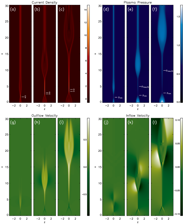
Figure 1: (Color online) Contour plots showing: (a)–(c) the out-of-plane current density, $J_{y}$, (d)–(f) the plasma pressure, $p$, (g)–(i) the outflow component of velocity, $V_{x}$, and (j)–(l) the inflow component of velocity, $V_{z}$, at times $22$, $44$, and $66$ for one of the two reconnection regions during the simulation of X-line retreat discussed in Sec. IV. The locations of the magnetic field null, flow stagnation point, pressure minimum along $z=0$, and pressure maximum within the current sheet are denoted by ‘n,’ ‘s,’ ‘$p_{\mathrm{min}}$,’ and ‘$p_{\mathrm{max,CS}}$,’ respectively.

Key features of the time evolution of the double perturbation simulation are shown in Fig. 1. The most apparent feature of the simulations is that the current sheets retreat from $x=0$ while the reconnection process is developing. The current sheet has a single wedge shape which is most apparent late in time. Figure 2(a) shows that the current sheet is thinnest near the magnetic field null, which is very close to the obstructed exit from the current sheet, and thickest near the obstructed exit.

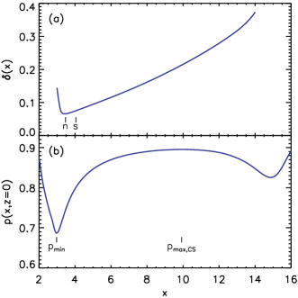
Figure 2: (Color online) Shown above at $t=66$ are (a) the current sheet thickness $\delta$ as a function of $x$, calculated as the half width at quarter maximum of $J_{y}$, and (b) the plasma pressure along $z=0$. In (a), the magnetic field null is denoted by ‘n’ and the flow stagnation point is denoted by ‘s,’ with $x_{n}=3.47$ and $x_{s}=4.05$. In (b), the global pressure minimum along $z=0$ and the pressure maximum within the current sheet are denoted by ‘$p_{\mathrm{min}}$’ and ‘$p_{\mathrm{max,CS}}$,’ respectively, with $x_{p,\mathrm{min}}=2.98$ and $x_{p,\mathrm{max,CS}}=9.90$.

As seen in Figs. 1(d)–(f), the peak plasma pressure in the magnetic island around $x=0$ is greater than the peak plasma pressure in the downstream region away from $x=0$. The plasma pressure gradient associated with the obstructing magnetic island is stronger and more localized than the plasma pressure gradient associated with the unobstructed outflow region. Early in time ($t\lesssim 20$), the X-point is located near the minimum of plasma pressure along $z=0$. Later ($20\lesssim t\lesssim 28$), the plasma pressure at the flow stagnation point is less than at the X-point. A local maximum of plasma pressure appears at $t\approx 27$ in the central region of the current sheet which persists through the remainder of the simulation. This pressure maximum is located slightly closer to the unobstructed exit of the current sheet than the obstructed exit.

Contours of the outflow component of velocity presented in Figs. 1(g)–(i) show that the outflow jet directed away from the obstruction is faster and longer than the outflow jet directed towards the obstruction. This behavior is consistent with previous simulations of asymmetric outflow reconnection.Roussev et al. (2001); Galsgaard and Roussev (2002); Oka et al. (2008); Zhu et al. (2009); Nakamura et al. (2010); Reeves et al. (2010) The kinetic energy and enthalpy fluxes away from the obstruction are much greater than the those towards the obstruction.

The inflow component of velocity is shown in Figs. 1(j)–(l). In the upstream regions outside the current sheet, the inflow component of velocity is roughly uniform except near the outflow region furthest from $x=0$. The inflow velocity late in time is $\sim$$0.015$–$0.02$. Because the large outflow blob from the unobstructed exit of the current sheet seen in Fig. 1 is propagating away from $x=0$, there is a quadrupole-like pattern for $V_{z}$ as upstream plasma ahead of the blob moves out of the way and upstream plasma behind the blob is pulled back towards $z=0$.

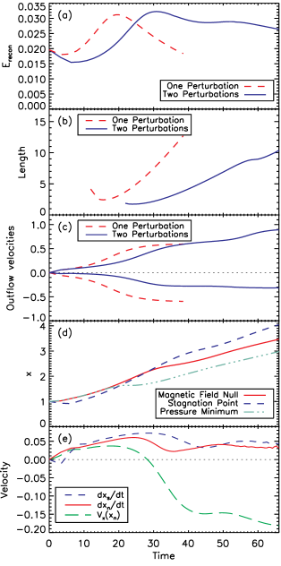
Figure 3: (Color online) Simulation results showing as a function of time (a) the reconnection electric field strength measured at the X-point, (b) the full length at quarter maximum of $J_{y}$ along $z=0$, (c) the peak outflow velocities, (d) the positions of the magnetic field null, flow stagnation point, and pressure minimum along $z=0$ ($x_{n}$, $x_{s}$, and $x_{p,\mathrm{min}}$, respectively), and (e) the rates of change in position of the magnetic field null and flow stagnation point ($\mathrm{d}x_{n}/\mathrm{d}t$ and $\mathrm{d}x_{s}/\mathrm{d}t$, respectively) and the velocity at the magnetic field null, $V_{x}(x_{n})$.

Figure 3 shows the time evolution of key quantities from the double perturbation simulation with comparisons to the otherwise equivalent single perturbation simulation used as a control for this study. Because a magnetic island forms at $t\approx 38$ in the single perturbation simulation, the comparison is halted at that time. Figure 3(a) shows the reconnection electric field strength for both simulations. The reconnection rate peaks more quickly in the single perturbation simulation than the double perturbation simulation. The development of reconnection in the double perturbation simulation is slow because the magnetic field null is located near the global pressure minimum along $z=0$ for $t\lesssim 20$ [see Fig. 3(d)] so that pressure gradients oppose outflow instead of facilitating it. However, the amplitude of the reconnection rate is eventually greater in the double perturbation case because the current sheet can increase in length in only one direction. As seen in Fig. 3(b), the single perturbation current sheet is a factor of $\sim$$2$–$3$ longer at any given time. The slight disturbances around $t\gtrsim 58$ in Figs. 3(a) and 3(b) may be due to the periodic boundary condition. While the reconnection rate is enhanced slightly in the double perturbation case, the difference is less than a factor of two so we conclude that the reconnection rate is only modestly affected by asymmetry or current sheet motion (see also Refs. Murphy et al., 2010 and Oka et al., 2008).

The peak outflow velocities in the positive and negative directions are shown in Fig. 3(c). Again, it is apparent that the double perturbation simulation takes longer to develop than the single perturbation simulation. The unobstructed outflow jet is typically $\sim$$2$–$3$ times faster than the obstructed outflow jet.

IV.2 The internal structure of the current sheet

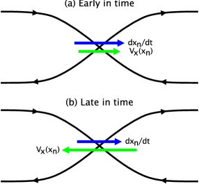
Figure 4: (Color online) A schematic showing the rate of X-line retreat, $\mathrm{d}x_{n}/\mathrm{d}t$, and the plasma flow velocity at the X-line, $V_{x}(x_{n})$. Early in time, both velocities are in the same direction. Late in time, there is significant plasma flow across the X-line in the opposite direction of X-line retreat.

The positions of the magnetic field null, flow stagnation point, and pressure minimum along $z=0$ ($x_{n}$, $x_{s}$, and $x_{p,\mathrm{min}}$, respectively) are presented in Fig. 3(d). The positions of the X-point and flow stagnation point are separated by a short distance. Both points are located very close to the obstructed exit of the current sheet. Early in time, the flow stagnation point is closer to the obstruction than the magnetic field null (e.g., $x_{s}<x_{n}$). This corresponds to the plasma flow at the X-line moving in the same direction as X-line retreat. Such a scenario is what one would expect if the frozen-in condition is approximately met [see Fig. 4(a)]. However, around $t\approx 28$ the relative positions of the magnetic field null and flow stagnation point switch (e.g., $x_{s}>x_{n}$). Hence at late times during this simulation the plasma flow at the X-line is in the opposite direction of X-line retreat [see Fig. 4(b)]. The peak resistive electric field in the double perturbation simulation occurs slightly after the time when $x_{n}=x_{s}$ (e.g., near the time when tension forces entirely work towards accelerating outflow rather than partially working against it).

The relative positions of the X-line and flow stagnation point switch because during near steady conditions, the flow stagnation point will in general be located near where the tension and pressure gradient forces cancel (e.g., Ref. Murphy et al., 2010). This implies that the total pressure at the flow stagnation point should be greater than the total pressure at the X-point when time-dependent effects are not important. Early in time ($t\lesssim 20$), the X-point is located very near the global pressure minimum along $z=0$ [see Fig. 3(d)]. During this phase, $p(x_{s})>p(x_{n})$ and the pressure gradient and tension forces at the flow stagnation point are oppositely directed. As the simulation progresses, the X-line and flow stagnation point retreat more quickly than the position of this pressure minimum. For $20\lesssim t\lesssim 28$, $p(x_{s})<p(x_{n})$ and the tension and pressure gradient forces at the flow stagnation point are pointed in the same direction and thus cannot cancel each other out. The flow stagnation point retreats quickly until $x_{n}<x_{s}$ and $p(x_{s})>p(x_{n})$ once again and for the remainder of the simulation [see Fig. 2(b)].

Figure 3(e) compares the rate of change in position of the magnetic field null $\mathrm{d}x_{n}/\mathrm{d}t$, the rate of change in position of the flow stagnation point $\mathrm{d}x_{s}/\mathrm{d}t$, and the plasma flow velocity across the magnetic field null $V_{x}(x_{n})$. As discussed in Ref. Seaton, 2008 and Sec. V, any difference between $V_{x}(x_{n})$ and $\mathrm{d}x_{n}/\mathrm{d}t$ must be due to resistive diffusion. The X-line is observed to retreat at a variable velocity ranging between $0.02$ and $0.06$. The flow stagnation point retreats more quickly than the magnetic field null for most of the simulation with velocities ranging from $0.03$ to $0.07$. For much of the first third of the simulation, $\mathrm{d}x_{s}/\mathrm{d}t\sim\mathrm{d}x_{n}/\mathrm{d}t\sim V_{x}(x_{n})$. When $x_{s}\approx x_{n}$, the rate of X-line retreat drops by a factor of $\sim$$3$ before slowly increasing and stabilizing. Following a delay after the drop in $\mathrm{d}x_{n}/\mathrm{d}t$, $\mathrm{d}x_{s}/\mathrm{d}t$ declines also before stabilizing. However, the most striking feature of Fig. 3(e) is that late in time there is significant plasma flow across the X-line in the opposite direction of X-line retreat: $V_{x}(x_{n})\sim-0.16$ while $\mathrm{d}x_{n}/\mathrm{d}t\sim 0.04$.

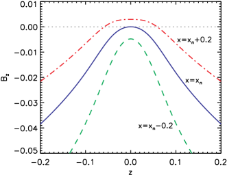
Figure 5: (Color online) The normal component of the magnetic field as a function of $z$ for three locations surrounding the magnetic field null at $t=66$. At $x=x_{n}$, $B_{z}<0$ in the vicinity of the current sheet except at $z=0$.

Figure 5 shows $B_{z}(z)$ for three locations surrounding the magnetic field null. Along $x=x_{n}$, $B_{z}<0$ except at $z=0$. Additionally, $\partial^{2}B_{z}/\partial t^{2}<0$ in the vicinity of the X-point. This magnetic field structure near the X-point can be seen clearly in the magnetic flux contour plot presented in Fig. 6, where magnetic field lines are pinched inward towards the right of the X-point. As we shall see in Sec. V, these features facilitate X-line retreat by diffusion of the normal component of the magnetic field in the inflow direction.

Figure 6: (Color online) Magnetic flux contours near the magnetic field null at $t=66$. The dotted line represents $x=x_{n}$.

Plasma flow at the X-line in the direction opposite to X-line retreat appears to be a persistent feature for the assumed configuration. This effect occurs during analogous simulations with initial uniform guide fields up to at least $B_{y0}=4$, a line-tied boundary at $x=0$, $\beta_{0}$ at least between $0.25$ and $4$, different diffusivities, and different initial separations at least for $\Delta<8$. During some of these simulations, an additional X-line appears near the leading end of the current sheet. For larger $\Delta$, the developing current sheets may become unstable to the plasmoid instabilityLoureiro et al. (2007); Samtaney et al. (2009); Bhattacharjee et al. (2009); Huang and Bhattacharjee (2010); Ni et al. (2010); Shepherd and Cassak (2010) before the retreat process begins. Plasma flow across the X-line in the direction opposite to X-line retreat does occasionally occur during analogous resistive MHD simulations of multiple competing reconnection sites, but less frequently because current sheet motion is inhibited.Young (2010)

IV.3 Components of the electric field and momentum balance

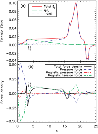
Figure 7: (Color online) Simulation results showing (a) components of the electric field and (b) force density contributions along $z=0$ at $t=66$. The magnetic field null is denoted by ‘n’ and the flow stagnation point is denoted by ‘s.’

Components of the out-of-plane electric field along $z=0$ are shown in Fig. 7(a) for $t=66$. This is late in the simulation when reconnection is well-developed and $x_{n}<x_{s}$. Inside the current sheet ($3\lesssim x\lesssim 14$), the electric field is approximately uniform but increases slightly with distance from $x=0$. The resistive electric field peaks in between the magnetic field null and flow stagnation point. In the obstructed outflow region, the electric field drops to a fraction of the value from inside the current sheet. From Faraday’s law, the positive slope of $E_{y}$ indicates that $B_{z}$ in the obstructing magnetic island is increasing with time. In the unobstructed outflow region, $E_{y}$ peaks sharply. This signature is indicative of the unobstructed downstream plasmoid being advected away from $x=0$.

Figure 7(b) shows force density contributions from the momentum equation (Eq. 4) along $z=0$ at $t=66$. Contributions include the magnetic tension force $B_{z}\partial B_{x}/\partial z$, the magnetic pressure gradient force $-\partial(B_{z}^{2}/2)/\partial x$, and the plasma pressure gradient force $-\partial p/\partial x$. Viscous forces are small and not shown explicitly, but are included in the calculation for total force density. The outflow towards the unobstructed exit is accelerated primarily by magnetic tension, whereas the outflow towards $x=0$ is accelerated primarily by the pressure gradient force. Intuitively, this is because the X-line is located very near one end of the current sheet so that the tension force directed towards that end is small and the tension force directed away from that end is large (e.g., Ref. Murphy and Sovinec, 2008). The force density at the flow stagnation point is negative until $t\approx 39$ when it becomes positive for the remainder of the simulation.

V THE RATE OF X-LINE RETREAT

This section contains a derivation of the rate of X-line retreat in the two-dimensional case. The geometry is assumed to be the same as that of the simulations reported in this paper. In particular, symmetry is assumed about $z=0$ so that the motion of the X-line is purely in the $x$ direction. No assumptions are made about the presence or absence of a guide field, except that $\partial/\partial y\rightarrow 0$. The analysis presented in this section can also be applied to the asymmetric inflow case by switching the inflow and outflow directions (see also Ref. Cassak and Shay, 2009).

The derivation of the rate of retreat of the X-line begins with Faraday’s law,

$$\frac{\partial\mathbf{B}}{\partial t}=-\nabla\times\mathbf{E}.$$ (11)

Evaluating the $z$-component of this expression and using the assumption of symmetry in the out-of-plane direction gives

$$\frac{\partial B_{z}}{\partial t}=-\frac{\partial E_{y}}{\partial x}.$$ (12)

Next, the convective derivative of $B_{z}$ at the X-point taken using the velocity of X-line retreat $\mathrm{d}x_{n}/\mathrm{d}t$ is given by

$$\left.\frac{\partial B_{z}}{\partial t}\right|_{x_{n}}+\frac{\mathrm{d}x_{n}}{\mathrm{d}t}\left.\frac{\partial B_{z}}{\partial x}\right|_{x_{n}}=0.$$ (13)

The right hand side of Eq. 13 is zero because the normal component of the magnetic field at the X-point does not change from zero, by definition. The rate of X-line retreat then follows from Eqs. 12 and 13 and is given by

$$\frac{\mathrm{d}x_{n}}{\mathrm{d}t}=\left.\frac{\partial E_{y}/\partial x}{\partial B_{z}/\partial x}\right|_{x_{n}}.$$ (14)

Intuitively, this means that the X-line moves in the direction of increasing reconnection electric field strength. This expression shows that it is not self-consistent to assume that the X-line is moving while the out-of-plane electric field is constant in space (cf. Ref. Owen and Cowley, 1987; *owen:1987:467).

This derivation has thus far not specified an expression for the out-of-plane electric field. By using the resistive MHD Ohm’s law $\mathbf{E}+\mathbf{V}\times\mathbf{B}=\eta\mathbf{J}$, Eq. 14 yields

$$\frac{\mathrm{d}x_{n}}{\mathrm{d}t}=V_{x}(x_{n})-\eta\left[\frac{\frac{\partial^{2}B_{z}}{\partial x^{2}}+\frac{\partial^{2}B_{z}}{\partial z^{2}}}{\frac{\partial B_{z}}{\partial x}}\right]_{x_{n}}.$$ (15)

For the assumed geometry, this is an exact result for resistive MHD. This analysis can be extended to include additional terms in the generalized Ohm’s law. The inverse dependence on $\left.\partial B_{z}/\partial x\right|_{x_{n}}$ in the resistive term comes from the geometric properties of Eq. 13; it is easier to change the position of a root of a function by a vertical shift if the slope of the function near the root is shallow. Because $\left.\partial^{2}B_{z}/\partial x^{2}\right|_{x_{n}}$ will usually be small if $\left.\partial B_{z}/\partial x\right|_{x_{n}}$ is small, it is likely that in resistive MHD the term $\left.\partial^{2}B_{z}/\partial z^{2}\right|_{x_{n}}$ representing diffusion of the normal component of the magnetic field in the inflow direction will be more important than the term $\left.\partial^{2}B_{z}/\partial x^{2}\right|_{x_{n}}$ representing diffusion of the normal component of the magnetic field along the outflow direction. Indeed, the simulation does show that late in time $\left.\partial^{2}B_{z}/\partial x^{2}\right|_{x_{n}}\ll\left.\partial^{2}B_{z}/\partial z^{2}\right|_{x_{n}}$. When the X-line is retreating during collisionless reconnection, it is possible that the term $\partial^{2}B_{z}/\partial x^{2}$ will become more important. During three-dimensional reconnection, the term $\partial^{2}B_{z}/\partial y^{2}$ may also play a role in facilitating X-line retreat.

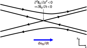
Figure 8: (Color online) The mechanism for X-line retreat due to diffusion of the normal component of the magnetic field in the inflow direction.

The mechanism for diffusion of the X-line is presented in Fig. 8. Along $x=x_{n}$, $B_{z}<0$ except at $z=0$. Then because $\partial^{2}B_{z}/\partial z^{2}<0$, the normal component of the magnetic field becomes more negative in the immediate vicinity of the X-point. This diffusion of $B_{z}$ in the $z$ direction causes the magnitude of $B_{z}$ to become stronger immediately to the left of the X-point and weaker immediately to the right of the X-point in Fig. 8. As a consequence, the X-point retreats to the right. The necessary features for this diffusion mechanism are apparent in Figs. 5 and 6. The contribution to X-line motion from diffusion of the normal component of the magnetic field in the outflow direction is not shown in Fig. 8.

The difference between the bulk plasma flow across the X-line, $V_{x}(x_{n})$, and the rate in change of position of the X-line, $\mathrm{d}x_{n}/\mathrm{d}t$, is subtle but important. In the ideal MHD limit, the magnetic field will be purely frozen in to the plasma so that these two quantities will be identical [e.g., $V_{x}(x_{n})=\mathrm{d}x_{n}/\mathrm{d}t$]. In this limit the X-line is purely advected by the bulk plasma flow. Therefore, any difference between $V_{x}(x_{n})$ and $\mathrm{d}x_{n}/\mathrm{d}t$ must be due to resistive diffusion of the magnetic field (see also Ref. Seaton, 2008).

The relation presented in Eq. 15 and Fig. 8 shows that the rate of X-line retreat depends fundamentally on local parameters near the X-point. Hence global models attempting to describe the rate of X-line retreat must take into account the coupling between large scales and the local structure of the magnetic field near the X-point. A starting point for such models may be the analysis presented in Ref. Shibata and Tanuma, 2001.

VI DISCUSSION AND CONCLUSIONS

This paper presents a resistive MHD simulation of two competing reconnection sites which move apart from each other as they develop. This investigation provides insight into the impact of current sheet motion on the reconnection process as well as on what happens when outflow from one exit of the current sheet is blocked.

The asymmetry in the reconnection process is most apparent in the outflow velocity profile. When the reconnection process is well-developed, the unobstructed outflow jet is $\sim$$2$–$3$ times faster than the obstructed outflow jet. As a consequence, most of the mass, energy, and momentum flux associated with the outflow is directed away from the obstructing magnetic island that forms between the two current sheets. Late in time, the reconnection rate is slightly higher in the double perturbation simulation than in an otherwise equivalent single perturbation simulation because the obstruction prevents the length of each current sheet from growing in one direction.

The X-point and flow stagnation point are both located very near the obstructed exit of the current sheet. This gives the reconnection layer a characteristic single wedge shape which is especially apparent late in time. During recent simulations of the plasmoid instability,Loureiro et al. (2007); Samtaney et al. (2009); Bhattacharjee et al. (2009); Huang and Bhattacharjee (2010); Ni et al. (2010); Shepherd and Cassak (2010) single wedge shaped small-scale reconnection sites are routinely observed with the X-point located near the thinnest part of the current sheet (see the online movie associated with Fig. 3 of Ref. Huang and Bhattacharjee, 2010). Because the X-line is located very close to one end of the current sheet, the tension force is directed predominantly towards the other direction (see also Refs. Murphy and Sovinec, 2008 and Galsgaard and Roussev, 2002). As in previous simulations of reconnection with asymmetric inflowCassak and Shay (2007, 2008, 2009); La Belle-Hamer et al. (1995); Ugai (2000); Kondoh et al. (2004); Borovsky and Hesse (2007); Birn et al. (2008); Pritchett (2008); Birn et al. (2010); Murphy and Sovinec (2008) and asymmetric outflow,Oka et al. (2008); Murphy and Sovinec (2008); Murphy et al. (2010) the X-line and flow stagnation point are separated by a short distance. This separation appears to be a ubiquitous feature of asymmetric reconnection.

The X-line retreats at speeds of $\sim$$0.02$–$0.06$ and the flow stagnation point retreats at speeds of $\sim$$0.03$–$0.07$. This is slower than the X-line retreat speed of $\sim$$0.1$ observed in Ref. Oka et al., 2008. Early in time, the plasma flow at the X-line is in the same direction as the rate in change of position of the X-line. While the reconnection process is still developing, however, the relative positions of the X-line and flow stagnation point switch. As a consequence, late in time the plasma flow at the X-line is in the opposite direction of X-line retreat. This switch occurs so that the flow stagnation point will be located near where the magnetic tension and plasma pressure forces cancel.

To further understand these results, an expression is derived for the rate of X-line retreat. In the assumed geometry, the X-line retreats in the direction of increasing reconnection electric field strength. In the resistive MHD limit, the X-line retreats due to either advection by the bulk plasma flow or by diffusion of the normal component of the magnetic field.

Interestingly, previous PIC simulations show that while the ion flow at the X-point is in the same direction as X-line retreat, the electron flow at the X-point is in the opposite direction (see Fig. 1 of Ref. Oka et al., 2008). Because in Hall MHD the magnetic field is frozen into the electron fluid rather than the bulk plasma, this result suggests that a similar effect occurs in fully kinetic simulations. It will be important in future work to determine whether or not this class of behavior occurs in more realistic geometries such as CME current sheets and the Earth’s magnetotail, or for substantially different plasma parameters.

The simulation presented in this paper can be used to assess the validity of the assumptions made by the steady-state model of reconnection with asymmetry in the outflow direction presented in Ref. Murphy et al., 2010. In particular, two assumptions require refinement. The first assumption is that the magnetic tension force contributes evenly to outflow from both sides. In the simulation, however, the tension force is almost entirely directed towards the unobstructed downstream region because the X-line is located very close to the obstructed exit. The second assumption is that the current sheet has approximately uniform thickness along the outflow direction. However, Figs. 1(c) and 2(a) show that the current sheet has a characteristic single wedge shape. Consequently, models for asymmetric outflow reconnection will need to be refined to account for these effects.

The results of this paper may have several implications for current sheets that form in the wakes of CMEs. In these events, the locations of the predominant X-line and flow stagnation point are expected to be located near the base of the current sheet (see also Refs. Savage et al., 2010, Reeves et al., 2010, and Seaton, 2008). Consequently, the mass, momentum, and energy fluxes are expected to be greater in the antisunward direction. This may provide an explanation for some of the observed properties of CMEs: that the masses of CMEs increase after leaving the Sun,Bemporad et al. (2007); Vourlidas et al. (2010); Lin et al. (2004) and that CMEs are heated even after leaving the flare site.Akmal et al. (2001); Ciaravella et al. (2001); Lee et al. (2009); Landi et al. (2010) Additionally, current sheets behind CMEs are expected to be thinner when observed at low altitudes and thicker when observed at high altitudes (e.g., compare the inferred thicknesses in Refs. Ciaravella and Raymond, 2008 and Savage et al., 2010). However, more observational and theoretical work is necessary before drawing conclusions. A complicating factor is that CME current sheets may be susceptible to the tearingFurth et al. (1963); Lin et al. (2007) and plasmoidLoureiro et al. (2007); Samtaney et al. (2009); Bhattacharjee et al. (2009); Huang and Bhattacharjee (2010); Ni et al. (2010); Shepherd and Cassak (2010) instabilities.

Effects associated with competition between multiple competing reconnection sites are likely to have consequences on the physics of turbulent reconnection. The model for turbulent reconnection by Lazarian and VishniacLazarian and Vishniac (1999) assumes that outflows from each of the small-scale reconnection sites in a large-scale current sheet do not significantly affect other reconnection sites. The two-dimensional simulations reported in this paper cannot fully address this problem. Hence in future work we will perform three-dimensional simulations with the initial perturbations offset from each other in the out-of-plane direction.

The resistive MHD simulations presented in this paper are not directly applicable to magnetic reconnection in the Earth’s magnetotail. There, two-fluid and collisionless effects not included in the resistive MHD framework are known to be important. Fully kinetic simulations such as those presented in Ref. Oka et al., 2008 show many of the same features as the double perturbation simulation presented here. Moreover, the shape and structure of the out-of-plane quadrupole magnetic field associated with two-fluid reconnection can be greatly affected by X-line retreat.Oka et al. (2008); Oka (2010) Hence, the NIMROD simulations reported in this paper will be extended to include two-fluid effects.