Fat Polygonal Partitions with Applications
to Visualization and Embeddings

Abstract

Let $\mathcal{T}$ be a rooted and weighted tree, where the weight of any node is equal to the sum of the weights of its children. The popular Treemap algorithm visualizes such a tree as a hierarchical partition of a square into rectangles, where the area of the rectangle corresponding to any node in $\mathcal{T}$ is equal to the weight of that node. The aspect ratio of the rectangles in such a rectangular partition necessarily depends on the weights and can become arbitrarily high.

We introduce a new hierarchical partition scheme, called a polygonal partition, which uses convex polygons rather than just rectangles. We present two methods for constructing polygonal partitions, both having guarantees on the worst-case aspect ratio of the constructed polygons; in particular, both methods guarantee a bound on the aspect ratio that is independent of the weights of the nodes.

We also consider rectangular partitions with slack, where the areas of the rectangles may differ slightly from the weights of the corresponding nodes. We show that this makes it possible to obtain partitions with constant aspect ratio. This result generalizes to hyper-rectangular partitions in ${\mathbb{R}}^{d}$. We use these partitions with slack for embedding ultrametrics into $d$-dimensional Euclidean space: we give a $\mathop{\rm polylog}(\Delta)$-approximation algorithm for embedding $n$-point ultrametrics into $\mathbb{R}^{d}$ with minimum distortion, where $\Delta$ denotes the spread of the metric, i.e., the ratio between the largest and the smallest distance between two points. The previously best-known approximation ratio for this problem was polynomial in $n$. This is the first algorithm for embedding a non-trivial family of weighted-graph metrics into a space of constant dimension that achieves polylogarithmic approximation ratio.

1 Introduction

Hierarchical structures are commonplace in many areas. It is not surprising, therefore, that the visualization of hierarchical structures—in other words, of rooted trees—is one of the most widely studied problems in information visualization and graph drawing. In the weighted variant of the problem, we are given a rooted tree in which each leaf has a positive weight and the weight of each internal node is the sum of the weights of the leaves in its subtree. One of the most successful practical algorithms for visualizing such weighted trees is the so-called Treemap algorithm. Treemap visualizes the given tree by constructing a hierarchical rectangular partition of a square, as illustrated in Figure 1(a). More precisely, Treemap assigns a rectangle to each node in the tree such that

• the area of the rectangle is equal to the weight of the node;

• the rectangles of the children of each internal node $\nu$ form a partition of the rectangle of $\nu$.

The Treemap algorithm was proposed by Shneiderman [21] and its first efficient implementation was given by Johnson and Shneiderman [14]. Treemap has been used to visualize a wide range of hierarchical data, including stock portfolios [15], news items [26], blogs [25], business data [24], tennis matches [13], photo collections [6], and file-system usage [21, 27]. Shneiderman maintains a webpage [20] that describes the history of his invention and gives an overview of applications and proposed extensions to his original idea. Below we only discuss the results that are directly related to our work.

In general, there are many different rectangular partitions corresponding to a given tree. To obtain an effective visualization it is desirable that the aspect ratio of the rectangles be kept as small as possible; this way the individual rectangles are easier to distinguish and the areas of the rectangles are easier to estimate. Various heuristics have been proposed for minimizing the aspect ratio of the rectangles in the partition [8, 22, 23]. Unfortunately, the aspect ratio can become arbitrarily bad if the weights have unfavorable values. For example, consider a tree with a root and two leaves, where the first leaf has weight 1 and the second has weight $W$. Then the optimal aspect ratio of any rectangular partition is unbounded as $W\rightarrow\infty$. Hence, in order to obtain guarantees on the aspect ratio we cannot restrict ourselves to rectangles. This lead Balzer et al. [2, 1] to introduce Voronoi treemaps, which use more general regions in the partition. However, their approach is heuristic and it does not come with any guarantees on the aspect ratio of the produced regions. Thus the following natural question is still open:

Suppose we are allowed to use arbitrary convex polygons in the partition, rather than just rectangles. Is it then always possible to obtain a partition that achieves aspect ratio independent of the weights of the nodes in the input tree? (The aspect ratio of a convex region $A$ is defined as $\operatorname{diam}(A)^{2}/\operatorname{area}(A)$, where $\operatorname{diam}(A)$ is its diameter and $\operatorname{area}(A)$ is its area.)

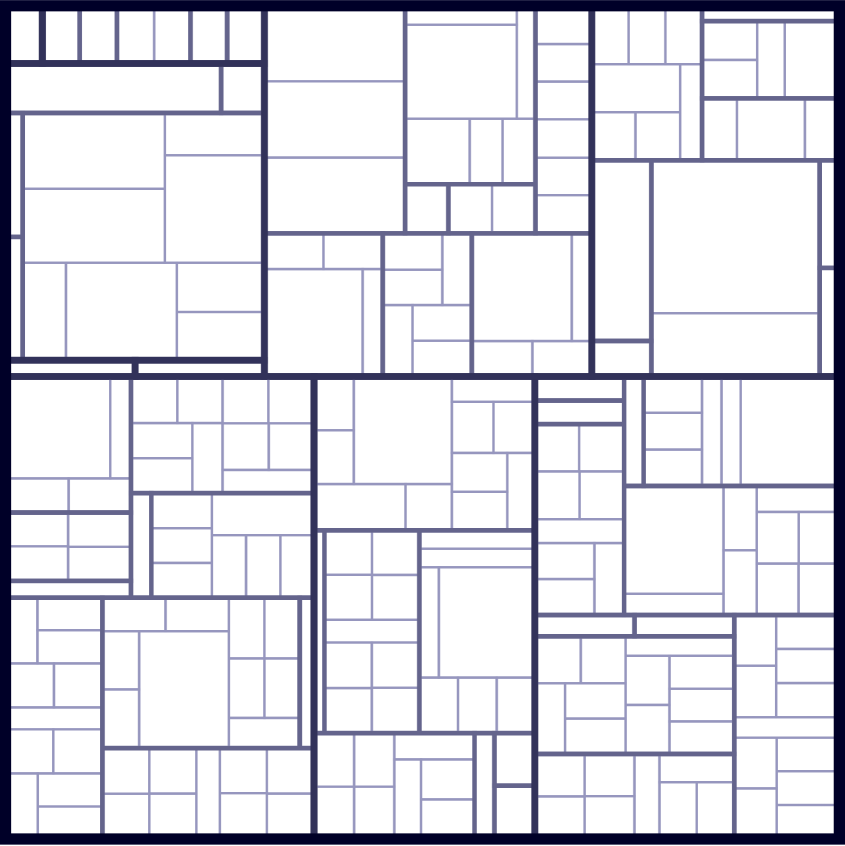
(a) A rectangular partition

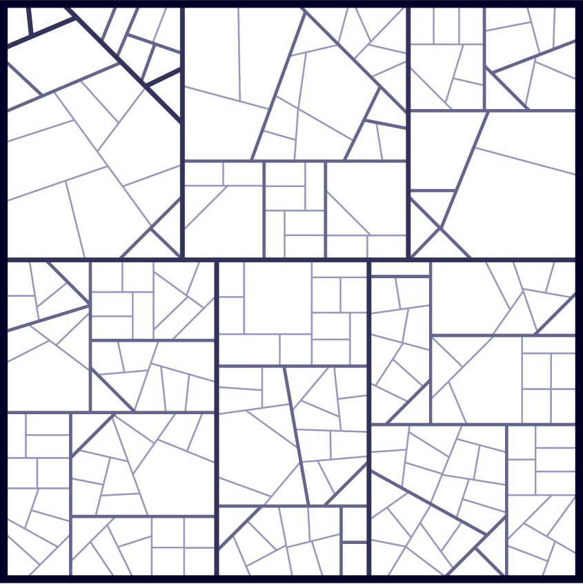
(b) A greedy polygonal partition

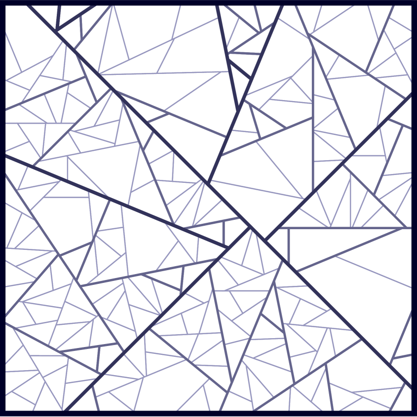
(c) An angular polygonal partition

Figure 1: Sample polygonal partitions

Our results on hierarchical partitions.

Our main result is an affirmative answer to the question above: we present two algorithms that, given an $n$-node tree of height $h$, construct a partition into convex polygons with aspect ratio $O(\mathop{\rm poly}(h,\log n))$. Our algorithms, which are described in Section 2, are very simple. They first convert the input tree into a binary tree, and then recursively partition the initial square region using straight-line cuts. The methods differ in the way in which the orientation of the cutting line is chosen at each step. The greedy method minimizes the maximum aspect ratio of two subpolygons resulting from the cut, while the angular method maximizes the angle that the splitting line makes with any of the edges of the polygon being cut. Figures 1(b) and 1(c) depict partitions computed by our algorithms.

The main challenge lies in the analysis of the aspect ratio achieved by the algorithms, which is given in Sections 3 and 4. We prove that the angular method produces a partition with aspect ratio $O(h+\log n)$. For the greedy method we can only prove an aspect ratio of $O((h+\log n)^{8})$. Since the greedy method is the most natural one, we believe this result is still interesting. Moreover, in the (limited) experiments we have done—see Section 2—the greedy method always outperforms the angular method. Besides these two algorithms, we also prove a lower bound: we show in Section 5 that for certain trees and weights, any partition into convex polygons must have polygons with aspect ratio $\Omega(h)$.

After having studied the problem of constructing polygonal partitions, we return to rectangular partitions. As observed, it is in general not possible to obtain any guarantees on the aspect ratio of the rectangles in the partition. If, however, we are willing to let the area of a rectangle deviate slightly from the weight of its corresponding node then we can obtain bounded aspect ratio, as we show in Section 6. More precisely, we obtain the following partition. Let $\varepsilon\in(0,1/3)$. We allow that the area $A$ of the rectangle assigned to every non-root node $v$ is shrunken by a factor of at most $1-\varepsilon$ compared to its share of the area $A^{\prime}$ of the rectangle of the parent $v^{\prime}$. That is, we only require that

$$(1-\varepsilon)\cdot\frac{A^{\prime}}{w_{v^{\prime}}}\leq\frac{A}{w_{v}}\leq\frac{A^{\prime}}{w_{v^{\prime}}},$$

where $w_{v}$ and $w_{v^{\prime}}$ are the weights of $v$ and $v^{\prime}$, respectively. Then we show that the aspect ratio of every rectangle can be bounded by $1/\varepsilon$. We call this kind of partition a rectangular partition with slack.

Application to embedding ultrametrics.

The work of Bădoiu et al. [9] establishes a lower bound for the distortion of the best embedding of an ultrametric into $\mathbb{R}^{d}$. Our hierarchical partitions with low aspect ratio can be used for efficiently constructing an embedding that closely matches the lower bound of Bădoiu et al. More details, including a brief history of relevant embedding results, follow.

Let us first recall a few standard definitions. A metric space $M=(X,D)$ is a set $X$ together with a symmetric distance function $D\colon X\times X\rightarrow{\mathbb{R}}_{\geq 0}$ that satisfies the triangle inequality and $D(x_{1},x_{2})=0$ if and only if $x_{1}=x_{2}$. An embedding of a metric space $M=(X,D)$ into a host metric space $M^{\prime}=(X^{\prime},D^{\prime})$ is an injective mapping $f\colon X\to X^{\prime}$. The distortion of an embedding $f$ is defined as

$$\max_{x,y\in X}\frac{D^{\prime}(f(x),f(y))}{D(x,y)}\cdot\max_{x,y\in X}\frac{D(x,y)}{D^{\prime}(f(x),f(y))}.$$

Over the past few decades, low-distortion embeddings of metric spaces into various host spaces have been the subject of extensive study [12]. Embeddings into Euclidean space are of particular importance in applications, and have received a lot of attention. Bourgain’s theorem [7] asserts that any $n$-point metric space admits an embedding into high-dimensional Euclidean space with distortion $O(\log n)$. Matoušek [16] has shown that the minimum distortion for embedding into $d$-dimensional Euclidean space is $n^{\Theta(1/d)}\cdot\log^{O(1)}n$. Since the distortion for embedding into constant-dimensional Euclidean space can be polynomially large in the worst case, it is natural to ask whether we can approximate the best possible distortion for a given input metric. Matoušek and Sidiropoulos [17] have shown that minimum-distortion embeddings of general metrics into ${\mathbb{R}}^{d}$ (with $d\geq 2$) are hard to approximate to within a factor of roughly $n^{1/(22d-10)}$, unless p=np [17]. In other words, it is unlikely that there exists a polynomial-time algorithm with significantly better performance than the worst case guarantee.

In light of the above inapproximability result, it is natural to ask whether there exist interesting families of metrics, for which we can obtain better than polynomial approximation factors for embedding into constant-dimensional Euclidean space. In this paper we present the first result of this type, for embedding ultrametrics into ${\mathbb{R}}^{d}$. An ultrametric is a metric satisfying the following strengthened version of the triangle inequality: for any $x,y,z\in X$ we have $D(x,z)\leq\max\{D(x,y),D(y,z)\}$. Equivalently, $M=(X,D)$ is an ultrametric if it can be realized as the shortest-path metric over the leaves of a rooted edge-weighted tree such that the distance between the root and any leaf is the same. Ultrametrics have received a lot of attention in the embeddings literature, and play a central role in many algorithmic applications (see e.g. [3]).

Bădoiu et al. [9] showed that finding a minimum-distortion embedding of an ultrametric into $\mathbb{R}^{2}$ is np-complete and presented an $O(n^{1/3})$-approximation algorithm for the problem. They extended the algorithm to embedding ultrametrics into $\mathbb{R}^{d}$, obtaining an $(n^{\frac{1}{d}-\Theta(\frac{1}{d^{2}})})$-approximation. This result is obtained using a lower bound on the amount of space required in a non-contracting embedding of every subtree of an ultrametric into $\mathbb{R}^{d}$. We apply our results on rectangular partitions with slack to a hierarchical structure corresponding to the ultrametric with weights given by the lower bound. Bounded aspect ratios in our partition imply relatively low distortion and good approximation to the best embedding of the ultrametric into $\mathbb{R}^{d}$. Moreover, we show a connection between embedding ultrametrics into ${\mathbb{R}}^{d}$ and (hyper-)rectangular partitions with slack and we use this connection to obtain a significant improvement over the result of Bădoiu et al. [9]. More precisely, using our results on (hyper-)rectangular partitions with slack, we obtain a polynomial-time $\mathop{\rm polylog}(\Delta)$-approximation algorithm for the problem of embedding ultrametrics into $(\mathbb{R}^{d},\ell_{2})$ with minimum distortion, where $\Delta$ is the spread of $X$. (The spread of $X$ is defined as $\Delta=\operatorname{diam}(X)/\min_{x,y\in X}D(x,y)$.) As long as the spread is sub-exponential in $n$, this is an exponential improvement over [9].

2 The two algorithms

Before we present our algorithms, we define the problem more formally and introduce some notation. Let $\mathcal{T}$ be a rooted tree. We say that $\mathcal{T}$ is properly weighted if each node $\nu\in\mathcal{T}$ has a positive weight $w(\nu)$ that equals the sum of the weights of the children of $\nu$. We assume without loss of generality that $w(\operatorname{root}(\mathcal{T}))=1$. A polygonal partition for a properly weighted tree assigns a convex polygon $P(\nu)$ to each node $\nu\in\mathcal{T}$ such that

• the polygon $P(\operatorname{root}(\mathcal{T}))$ is the unit square;

• for any node $\nu$ we have $\operatorname{area}(P(\nu))=w(\nu)$;

• for any node $\nu$, the polygons assigned to the children of $\nu$ form a disjoint partition of $P(\nu)$.

Recall that the aspect ratio of a planar convex region $A$, denoted by $\operatorname{asp}(A)$, is defined as $\operatorname{asp}(A):=\operatorname{diam}(A)^{2}/\operatorname{area}(A)$. The aspect ratio of a polygonal partition is the maximum aspect ratio of any of the polygons in the partition. Our goal is to show that any properly weighted tree admits a fat polygon partition, that is, a polygonal partition with small aspect ratio.

We propose two methods for constructing fat polygonal partitions. They both start with transforming the input tree $\mathcal{T}$ into a binary tree $\mathcal{T}^{\prime}$. The nodes of $\mathcal{T}$ are a subset of nodes of $\mathcal{T}^{\prime}$, and two nodes are in the ancestor-descendant relation in $\mathcal{T}$ if and only if they are in the same relation in $\mathcal{T}^{\prime}$. The weights assigned to nodes of $\mathcal{T}$ are preserved in $\mathcal{T}^{\prime}$. Any polygonal partition for $\mathcal{T}^{\prime}$ restricted to nodes from $\mathcal{T}$ is a polygonal partition for $\mathcal{T}$. Then, for the binary tree $\mathcal{T}^{\prime}$, it suffices to design a method that cuts the polygon $P(\nu)$ corresponding to a node $\nu$ into two polygons of prespecified areas that correspond to $\nu$’s children. We propose two such methods: the angular method and the greedy method. To achieve a polygonal partition for $\mathcal{T}^{\prime}$, it suffices to recursively apply one of the cutting methods.

The transformation into a binary tree.

We transform the input $n$-node tree $\mathcal{T}$ into a binary tree $\mathcal{T}^{\prime}$ by replacing every internal node $\nu$ of degree greater than two by a collection of nodes whose subtrees together are exactly the subtrees of $\nu$. This can be done in such a way that $\operatorname{height}(\mathcal{T}^{\prime})=O(\operatorname{height}(\mathcal{T})+\log n)$ [19]. The number of nodes in $\mathcal{T}^{\prime}$ is $O(n)$. For completeness we sketch how this transformation is done.

For a node $\nu$, we use $\mathcal{T}_{\nu}$ to denote the subtree rooted at $\nu$, and $|\mathcal{T}_{\nu}|$ to denote the number of nodes in $\mathcal{T}_{\nu}$. The transformation is a recursive process, starting at the root of $\mathcal{T}$. Suppose we reach a node $\nu$. If $\nu$ has degree two or less, we just recurse on the at most two children of $\nu$. If $\nu$ has degree $k\geq 3$, we proceed as follows. Let $C(\nu)$ be the set of children of $\nu$, and let $\mu\in C(\nu)$ be the child with the largest number of nodes in its subtree. We partition $C(\nu)\setminus\{\mu\}$ into two non-empty subsets $C_{1}(\nu)$ and $C_{2}(\nu)$ such that $\sum_{\mu\in C_{1}(\nu)}|\mathcal{T}_{\mu}|<|\mathcal{T}_{\nu}|/2$ and $\sum_{\mu\in C_{2}(\nu)}|\mathcal{T}_{\mu}|<|\mathcal{T}_{\nu}|/2$. We create three new nodes $\nu_{1},\nu_{2},\nu_{3}$ and modify the tree as shown in Figure 2. The weights $w(\nu_{1}),w(\nu_{2}),w(\nu_{3})$ are set to the sum of the weights of the leaves in their respective subtrees. Finally, we recurse on $\nu_{1}$, $\mu$, and $\nu_{3}$.

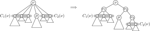
Figure 2: Transforming a tree to a binary tree.

After the procedure has finished we have a (properly weighted) tree in which every node has degree at most two. We remove all degree-1 nodes to obtain our binary tree $\mathcal{T}^{\prime}$. The height of $\mathcal{T}^{\prime}$ is at most $2(\operatorname{height}(\mathcal{T})+\log n)$, because every time we go down two levels in $\mathcal{T}^{\prime}$ we either pass through an original node from $\mathcal{T}$ or the number of nodes in the subtree halves.

Figure 3: Sample executions of our cutting methods.

Methods for cutting a polygon.

Suppose we have to cut a convex polygon $P(\nu)$ into two subpolygons. Note that if we fix an orientation for the cut, then there are only two choices left for the cut because the areas of the subpolygons are prespecified. (The two choices correspond to having the smaller of the two areas to the left or to the right of the cut.) Our cutting methods, depicted in Figure 3 are the following.

• Angular: Let $c$ denote the cut, that is, the line segment separating the two subpolygons of $P(\nu)$. We select the orientation of $c$ such that we maximize

  $$\min\{\operatorname{angle}(c,e):\hbox{$e$ is an edge of the input polygon}\},$$

  where $\operatorname{angle}(c,e)$ is the smaller of the angles between the lines $\ell(c)$ and $\ell(e)$ containing $c$ and $e$, respectively. In other words, we cut in a direction as different as possible from all the orientations determined by the edges of the polygon. We then take any of the two cuts of the selected orientation.

• Greedy: The greedy method selects the cut that minimizes the maximum of the aspect ratios of the two subpolygons.

Experiments.

To get an idea of the relative performance of the two methods we implemented them and performed some experiments. Table 1 shows the results on two hierarchies. One is synthetic and was generated using a random process, the other is the home directory with all subfolders of one of the authors. Leaves in the latter hierarchy are the files in any of the folders, and the weight of a leaf is the size of the corresponding file. For comparison, we also ran two additional partitioning methods. Both of these methods use the transformation of the input into a binary tree. The random method always makes a cut in a random direction. In the greedy rectangular method, all polygons are rectangles and all cuts are parallel to the sides of the original rectangle. The method always greedily chooses the cut that is perpendicular to the longer side, which maximizes the aspect ratio of the two subpolygons resulting from the cut.

Method	Synthetic Data		Home Folder
	Average	Maximum	Average	Maximum
Angular	3.79	13.19	3.87	20.11
Greedy	2.56	6.79	2.57	8.39
Random	5.79	355.14	6.26	1609.66
Greedy Rectangular	3.52	1445.99	24.49	230308.30

Table 1: Aspect ratios of partitions generated by various methods

In all our tests, the methods partitioned a square. The greedy method performs best, closely followed by the angular method. Interestingly, the greedy rectangular method performs even worse than the random method—apparently restricting to rectangles is a very bad idea as far as aspect ratio is concerned.

In the next two sections we prove that both the angular method and the greedy method construct a partition in which the aspect ratios are $O(\mathop{\rm poly}(\operatorname{height}{\mathcal{T}}+\log n))$. For the angular method, the proof is simpler and gives a better bound on the worst-case aspect ratio. We present the more complicated proof for the greedy method because it is the most natural method and it has the best performance in practice.

3 Analysis of angular partitions

The idea behind the angular partitioning method is that a polygon with large aspect ratio must have two edges that are almost parallel. Hence, if we avoid using partition lines whose orientations are too close to each other, then we can control the aspect ratio of our subpolygons. Next we make this idea precise.

Let $U$ be the initial unit square that we partition, and let $\phi>0$ be a parameter. Recall that for two line segments $e$ and $e^{\prime}$, we use $\operatorname{angle}(e,e^{\prime})$ to denote the smaller angle defined by the lines $\ell(e)$ and $\ell(e^{\prime})$ containing $e$ and $e^{\prime}$, respectively. We define a convex polygon $P\subset U$ to be a $\phi$-separated polygon if it satisfies the following condition. For any two distinct edges $e$ and $e^{\prime}$, we have:

1. $\operatorname{angle}(e,e^{\prime})\geq\phi$; or

2. $e$ is contained in $U$’s top edge and $e^{\prime}$ is contained in $U$’s bottom edge (or vice versa); or

3. $e$ is contained in $U$’s left edge and $e^{\prime}$ is contained in $U$’s right edge (or vice versa).

Lemma 1.

The aspect ratio of a $\phi$-separated polygon $P$ is $O(1/\phi)$.

Proof.

Let $d:=\operatorname{diam}(P)$ and let $uv$ be a diagonal of $P$ that has length $d$. Consider the bounding box $B$ of $P$ that has two edges parallel to $uv$. We call the edge of $B$ parallel to and above $uv$ its top edge, and the edge of $B$ parallel to and below $uv$ its bottom edge. Let $r$ be a vertex of $P$ on the top edge of $B$ and let $s$ be a vertex on its bottom edge—see Fig. 4.

Figure 4: Illustration for the proof of Lemma 1.

Let $e_{1}$ and $e_{2}$ be the edges of $P$ incident to $r$, and let $e_{3}$ and $e_{4}$ be the edges incident to $s$. Let the angles $\alpha_{1},\ldots,\alpha_{4}$ be defined as in Fig. 4. We distinguish two cases.

• Case (a): none of $e_{1},e_{2},e_{3},e_{4}$ are parallel.
  By condition (i), this implies that the angles any two edges make is at least $\phi$. Hence, we have

  $$\phi \leq\operatorname{angle}(e_{1},e_{3})\leq\max(\alpha_{1},\alpha_{3}),$$ (1)

  $$\phi \leq\operatorname{angle}(e_{2},e_{4})\leq\max(\alpha_{2},\alpha_{4}),$$ (2)

  $$\phi \leq\operatorname{angle}(e_{1},e_{4})\leq\alpha_{1}+\alpha_{4},$$ (3)

  $$\phi \leq\operatorname{angle}(e_{2},e_{3})\leq\alpha_{2}+\alpha_{3}.$$ (4)

  By (3) we have $\alpha_{1}+\alpha_{4}\geq\phi$. Now assume without loss of generality that $\alpha_{1}\geq\phi/2$. If $\alpha_{2}\geq\phi/2$ as well, then

  $$\operatorname{area}(uvr)\geq(d^{2}/4)\cdot\sin(\phi/2).$$

  Since $uvr\subset P$, this implies that

  $$\operatorname{asp}(P)\leq\frac{d^{2}}{(d^{2}/4)\cdot\sin(\phi/2)}=O(1/\phi).$$

  If $\alpha_{2}<\phi/2$, then we use (2) and (4) to conclude that $\alpha_{4}\geq\phi$ and $\alpha_{3}\geq\phi/2$. Hence, we now have $\operatorname{area}(uvs)\geq(d^{2}/4)\cdot\sin(\phi/2)$, which implies that $\operatorname{asp}(P)=O(1/\phi)$.

• Case (b): some edges in $e_{1},e_{2},e_{3},e_{4}$ are parallel.
  By conditions (i)–(iii), two edges of $P$ can be parallel only if they are contained in opposite edges of $U$. Hence, $|rs|\geq 1$. Moreover, since $uv$ defines the diameter we have $|uv|\geq|rs|$. Let $\alpha:=\operatorname{angle}(uv,rs)$, as illustrated in Fig. 5.

  

  Figure 5: The case of parallel edges.

  If $\alpha\geq\min\{\phi,\pi/4\}$, this is easily seen to imply that $\operatorname{area}(P)\geq\operatorname{area}(urvs)=\Omega(\phi)$, which means that $\operatorname{asp}(P)=O(1/\phi)$. Now consider the case where $\alpha<\phi$ and $\alpha<\pi/4$. We show that this leads to a contradiction. Let $x:=uv\cap rs$ and assume without loss of generality that, as in Figure 5, we have $\alpha=\angle rxv$. Then $\operatorname{angle}(e_{1},e_{3})\leq\alpha<\phi$. By conditions (i)–(iii) this can only happen if $e_{1}$ and $e_{3}$ are contained in opposite edges of $U$, if we assume that $r$ and $s$ are chosen such that they maximize the distances between $r$ and $s$, which can be done without loss of generality. We have $\operatorname{angle}(e_{3},rs)\leq\operatorname{angle}(uv,rs)=\alpha\leq\phi<\pi/4$. However, it is impossible to place two points $r$ and $s$ on opposite sides of $U$ such that $\operatorname{angle}(e_{3},rs)<\pi/4$. The smallest angle one can obtain is $\pi/4$.

∎

To construct a polygonal partition we use the procedure described in Section 2. Thus, we first transform the input tree $\mathcal{T}$ into a corresponding binary tree $\mathcal{T}^{\prime}$. Next, we recursively apply the angular cutting method to $\mathcal{T}^{\prime}$, that is, at each node $\nu$, we cut the polygon $P(\nu)$, using a cut $c$ that maximizes the minimum angle $c$ makes with any of the edges of $P(\nu)$.

Lemma 2.

Let $P(\nu)$ be the subpolygon generated by the algorithm above for a node $\nu$ at level $k$ in $\mathcal{T}^{\prime}$. Then $P(\nu)$ is a $(\pi/(2k+6))$-separated polygon.

Proof.

The proof is by induction on $k$.

For $k=0$, we have $\nu=\operatorname{root}(\mathcal{T}^{\prime})$ and $P(\nu)$ is a unit square. Hence, $P(\nu)$ is $(\pi/2)$-separated and therefore also $(\pi/6)$-separated.

For $k>0$ we argue as follows. By the induction hypothesis, the polygon $P(\mu)$ corresponding to the parent $\mu$ of $\nu$ is $(\pi/(2k+4))$-separated. Moreover, by construction it has at most $4+(k-1)=k+3$ edges. Consider the sorted (circular) sequence of angles that these edges make with the $x$-axis. By the pigeon-hole principle, there must be two adjacent angles that are at least $\pi/(k+3)$ apart. Hence, the cut $c$ that is chosen to partition $P(\mu)$ makes an angle at least $\pi/(2k+6)$ with all edges of $P(\mu)$, and by the induction hypothesis, all the other angles are at least $\pi/(2k+4)$. ∎

Recall that the height of the binary tree $\mathcal{T}^{\prime}$ is $O(\operatorname{height}(\mathcal{T})+\log n)$. Hence, we get the following theorem.

Theorem 1.

Let $\mathcal{T}$ be a properly weighted tree with $n$ nodes. Then the angular partitioning method constructs a polygonal partition for $\mathcal{T}$ whose aspect ratio is $O(\operatorname{height}(\mathcal{T})+\log n)$.

4 Analysis of greedy partitions

We now turn our attention to the greedy method, which at each step chooses a cut $c$ that minimizes the maximum aspect ratio of the two subpolygons resulting from the cut. The main component of our proof that polygonal partitions with good properties exist will be the following lemma. It shows that there is always a way to cut a polygon into two smaller polygons of required areas so that the aspect ratios of the new subpolygons are bounded.

Note that the lemma requires that the number of vertices in the polygon be bounded. If the number of vertices is unbounded, the polygon may become arbitrarily close to a circle. In this case there is no good cut if one of the resulting polygons has to be much smaller than the other.

The proof of the lemma is long and consists of a case analysis. An impatient reader may prefer to omit the proof and move directly to Theorem 2.

Lemma 3 (Good cuts).

Let $P\subset\mathbb{R}^{2}$ be a convex polygon with $k$ vertices, and let $a\in(0,1/2]$. Then $P$ can be partitioned into two convex polygons $P_{1}$ and $P_{2}$ such that

• Each of the $P_{1}$ and $P_{2}$ has at most $k+1$ vertices.

• $\operatorname{area}(P_{1})=a\cdot\operatorname{area}(P)$, and $\operatorname{area}(P_{2})=(1-a)\cdot\operatorname{area}(P)$.

• $\max\{\operatorname{asp}(P_{1}),\operatorname{asp}(P_{2})\}\leq\max\left\{\operatorname{asp}(P)\left(1+\frac{6}{k}\right),k^{8}\right\}$.

Proof.

We distinguish two cases, depending on whether $a\leq 1/k^{2}$ (that is, we are cutting off a relatively small subpolygon) or not.

Case 1: $a\leq 1/k^{2}$. Let $\phi$ be the smallest angle of $P$, and let $v$ be a vertex of $P$ whose interior angle is $\phi$. Since $P$ has $k$ vertices, we have

$$\phi\leq\pi\left(1-\frac{2}{k}\right).$$

Let $\ell$ be the angular bisector at $v$. Consider the cut $c$ orthogonal to $\ell$ such that $\operatorname{area}(P_{1})=a\cdot\operatorname{area}(P)$, where $P_{1}$ is the subpolygon induced by $c$ having $v$ as a vertex—see Figure 6(a) for an illustration. Let $P_{2}$ be the other subpolygon. Clearly, $P_{1}$ and $P_{2}$ are convex polygons of the required area with at most $k+1$ vertices each. Therefore, it remains to bound the aspect ratios of $P_{1}$ and $P_{2}$.

Since $P_{2}\subset P$, we have

$$\operatorname{asp}(P_{2}) =\frac{\operatorname{diam}(P_{2})^{2}}{\operatorname{area}(P_{2})}\leq\frac{\operatorname{diam}(P)^{2}}{(1-a)\cdot\operatorname{area}(P)}=\frac{\operatorname{asp}(P)}{1-a}<\operatorname{asp}(P)\left(1+2a\right)$$

$$<\operatorname{asp}(P)\left(1+\frac{2}{k^{2}}\right)<\operatorname{asp}(P)\left(1+\frac{1}{k}\right).$$

We next bound $\operatorname{asp}(P_{1})$. Let $x_{1},x_{2}$ be the two endpoints of the cut $c$, and let $t$ be the distance between $x_{1}$ and $x_{2}$. Let $h$ be the distance from $v$ to $c$. We distinguish between two subcases.

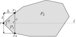
(a) Case 1.

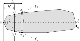
(b) Case 1.2.

Figure 6: Partitioning $P$ into $P_{1}$ and $P_{2}$ when $a\leq 1/k^{2}$.

Case 1.1: $t\geq h/k^{2}$. Since $P$ is convex, the triangle $vx_{1}x_{2}$ is contained in $P_{1}$. Therefore,

$$\operatorname{area}(P_{1})\geq h\cdot t/2\geq h^{2}/(2k^{2}).$$

On the other hand, since $c$ is normal to the bisector of the angle of $v$, it follows that $P_{1}$ is contained inside a rectangle of width $h$ and height $H$, with

$$H \leq 2\cdot h\cdot\tan(\phi/2)\leq 2\cdot h\cdot\tan\left(\frac{\pi(1-2/k)}{2}\right)$$

$$\leq 2\cdot h/\tan(\pi/k)\leq 2\cdot h\cdot k/\pi.$$

Thus, $\operatorname{diam}(P_{1})<h(1+2\cdot k/\pi)$. It follows that

$$\operatorname{asp}(P_{1})=\frac{\operatorname{diam}(P_{1})^{2}}{\operatorname{area}(P_{1})}<\frac{(h+2\cdot h\cdot k/\pi)^{2}}{h^{2}/(2k^{2})}<k^{5}.$$

Case 1.2: $t<h/k^{2}$. Let $\ell_{1}$ be the line passing through $v$ and $x_{1}$, and let $\ell_{2}$ be the line passing through $v$ and $x_{2}$. Let $\gamma$ be the angle between $\ell_{1}$ and $\ell_{2}$. Observe that $P_{2}$ is contained between $\ell_{1}$ and $\ell_{2}$. Therefore, if $u$ is the point in $P_{2}$ farthest away from $v$ we have

$$\frac{\gamma}{2\pi}\pi|uv|^{2}\geq\operatorname{area}(P_{2}),$$

where $|uv|$ denotes the length of the segment $uv$. It follows that

$$\operatorname{diam}(P)^{2}\geq|uv|^{2}\geq\frac{2}{\gamma}(1-a)\cdot\operatorname{area}(P).$$

Therefore,

$$\operatorname{asp}(P)=\frac{\operatorname{diam}(P)^{2}}{\operatorname{area}(P)}\geq\frac{2}{\gamma}\left(1-a\right)\geq\frac{2}{\gamma}\left(1-\frac{1}{k^{2}}\right).$$

We now give an upper bound on the diameter of $P_{1}$. Assume without loss of generality that $|vx_{2}|\geq|vx_{1}|$. Consider a segment $y_{1}y_{2}$ parallel to $x_{1}x_{2}$ with $y_{1},y_{2}\in\operatorname{\partial}P$ such that $y_{1}y_{2}$ lies between $x_{1}x_{2}$ and $v$—see Figure 6(b). Let $h^{\prime}$ be the distance between $v$ and $y_{1}y_{2}$. We first argue that $|y_{1}y_{2}|\leq 2t$.

Assume for the sake of contradiction that $|y_{1}y_{2}|>2t$. Let $g_{1}$ be the line passing through $y_{1}$ and $x_{1}$, and let $g_{2}$ be the line passing through $y_{2}$ and $x_{2}$. Observe that since $|y_{1}y_{2}|>|x_{1}x_{2}|$, the lines $g_{1}$ and $g_{2}$ intersect in a point $w$ such that $P_{2}$ is contained in the triangle $x_{1}x_{2}w$. Furthermore, the polygon $vy_{1}x_{1}x_{2}y_{2}$ is contained in $P_{1}$. If $h^{\prime}\geq h/2$, then the area of the triangle $vy_{1}y_{2}$ is greater or equal to the area of the triangle $x_{1}x_{2}w$. Therefore, $\operatorname{area}(P_{1})\geq\operatorname{area}(P_{2})$, contradicting the fact that $a\leq 1/k^{2}$. If, on the other hand, $h^{\prime}<h/2$, then the area of the quadrilateral $y_{1}x_{1}x_{2}y_{2}$, is greater than the area of the triangle $x_{1}x_{2}w$, again implying that $\operatorname{area}(P_{1})\geq\operatorname{area}(P_{2})$, a contradiction. Therefore, we obtain that $|y_{1}y_{2}|\leq 2t$.

It now follows that any point $q\in P_{1}$ is at distance at most $2t$ from the line segment $vx_{2}$. Moreover, we have $t<h/k^{2}\leq|vx_{2}|/k^{2}$. Hence,

$$\operatorname{diam}(P_{1})=\max_{q,q^{\prime}\in P_{1}}|qq^{\prime}|\leq 2t+|vx_{2}|+2t\leq|vx_{2}|\left(1+\frac{4}{k^{2}}\right).$$

Let $x^{*}$ be the point on the line segment $x_{1}x_{2}$ that is closest to $v$. Since $|vx_{2}|\geq h$, we have

$$\operatorname{area}(P_{1})\geq\frac{\gamma}{2\pi}\pi|vx^{*}|^{2}\geq\frac{\gamma}{2}(|vx_{2}|-t)^{2}\geq\frac{\gamma}{2}|vx_{2}|^{2}\left(1-\frac{1}{k^{2}}\right).$$

Therefore,

$$\operatorname{asp}(P_{1}) =\frac{\operatorname{diam}(P_{1})^{2}}{\operatorname{area}(P_{1})}\leq\frac{2}{\gamma}\cdot\frac{(1+4/k^{2})^{2}}{1-1/k^{2}}\leq\operatorname{asp}(P)\frac{(1+4/k^{2})^{2}}{(1-1/k^{2})^{2}}$$

$$\leq\operatorname{asp}(P)\cdot(1+6/k^{2})^{2}\leq\operatorname{asp}(P)\cdot(1+2/k)^{2}$$

$$\leq\operatorname{asp}(P)\cdot(1+6/k).$$

Case 2: $a>1/k^{2}$.

Case 2.1: $\operatorname{asp}(P)\leq k^{6}$. In this case any cut giving the two subpolygons $P_{1}$ and $P_{2}$ the required areas works. Indeed,

$$\operatorname{asp}(P_{1})=\frac{\operatorname{diam}(P_{1})^{2}}{\operatorname{area}(P_{1})}\leq\frac{\operatorname{diam}(P)^{2}}{a\cdot\operatorname{area}(P)}\leq k^{2}\cdot\operatorname{asp}(P)\leq k^{8}$$

and

$$\operatorname{asp}(P_{2})=\frac{\operatorname{diam}(P_{2})^{2}}{\operatorname{area}(P_{2})}\leq\frac{\operatorname{diam}(P)^{2}}{(1-a)\cdot\operatorname{area}(P)}\leq 2\cdot\operatorname{asp}(P)\leq 2\cdot k^{6}<k^{7}.$$

Case 2.2: $\operatorname{asp}(P)>k^{6}$. Pick points $v_{1},v_{2}\in P$, such that $|v_{1}v_{2}|=\operatorname{diam}(P)$. For each $z\in[0,\operatorname{diam}(P)]$, let $\ell(z)$ be a line normal to $v_{1}v_{2}$ that is at distance $z$ from $v_{1}$ and intersects $P$. Note that $\ell(0)$ contains $v_{1}$ and $\ell(\operatorname{diam}(P))$ contains $v_{2}$. Define $f(z)$ to be the length of the intersection of $P$ with $\ell(z)$. Observe that

$$\operatorname{area}(P)=\int_{z=0}^{\operatorname{diam}(P)}f(z)dz$$

Pick $s_{1},s_{2}\in[0,\operatorname{diam}(P)]$, so that

$$a\cdot\operatorname{area}(P)=\int_{z=0}^{s_{1}}f(z)dz=\int_{z=\operatorname{diam}(P)-s_{2}}^{\operatorname{diam}(P)}f(z)dz.$$

Let $Q_{1}$ be the part of $P$ that is contained between $\ell(0)$ and $\ell(s_{1})$. Similarly, let $Q_{2}$ be the part of $P$ that is contained between $\ell(\operatorname{diam}(P)-s_{2})$ and $\ell(\operatorname{diam}(P))$. Clearly, both $Q_{1}$ and $Q_{2}$ are convex polygons with at most $k+1$ vertices.

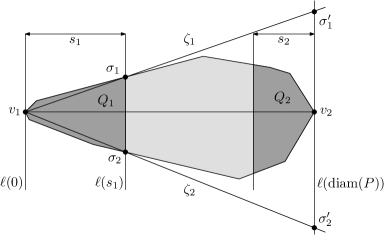
Figure 7: Partitioning $P$ into $P_{1}$ and $P_{2}$, when $\alpha>1/k^{2}$: Case 2.2.

First, we will show that

$$\min\left\{\frac{\operatorname{area}(Q_{1})}{s_{1}},\frac{\operatorname{area}(Q_{2})}{s_{2}}\right\}\leq\frac{\operatorname{area}(P)}{\operatorname{diam}(P)}$$

Assume for a contradiction that both $\operatorname{area}(Q_{1})/s_{1}$ and $\operatorname{area}(Q_{2})/s_{2}$ are greater than $\operatorname{area}(P)/\operatorname{diam}(P)$. It follows that there exist $z_{1}\in[0,s_{1}]$ and $z_{2}\in[\operatorname{diam}(P)-s_{2}]$ such that $f(z_{1})>\operatorname{area}(P)/\operatorname{diam}(P)$ and $f(z_{2})>\operatorname{area}(P)/\operatorname{diam}(P)$. Since $P$ is convex, $f$ is a bitonic function. Therefore, for each $z\in[z_{1},z_{2}]$, we have $f(z)>\operatorname{area}(P)/\operatorname{diam}(P)$. It follows that

$$\operatorname{area}(P)=\operatorname{area}(Q_{1})+\operatorname{area}(Q_{2})+\operatorname{area}(P\setminus(Q_{1}\cup Q_{2}))>\frac{\operatorname{area}(P)}{\operatorname{diam}(P)}\cdot\operatorname{diam}(P),$$

a contradiction.

We can therefore assume without loss of generality that

$$\frac{\operatorname{area}(Q_{1})}{s_{1}}\leq\frac{\operatorname{area}(P)}{\operatorname{diam}(P)}.$$

Note that this implies

$$s_{1}\geq a\cdot\operatorname{diam}(P).$$

We set $P_{1}=Q_{1}$, and $P_{2}=P\setminus Q_{1}$. It remains to bound $\operatorname{asp}(P_{1})$ and $\operatorname{asp}(P_{2})$.

By the convexity of $P$, we have

$$\operatorname{area}(P)\geq\max_{z\in[0,\operatorname{diam}(P)]}f(z)\cdot\operatorname{diam}(P)/2.$$

Since $\operatorname{asp}(P)>k^{6}$, it follows that

$$\max_{z\in[0,\operatorname{diam}(P)]}f(z)\leq 2\cdot\frac{\operatorname{area}(P)}{\operatorname{diam}(P)^{2}}\cdot\operatorname{diam}(P)<\frac{2}{k^{6}}\cdot\operatorname{diam}(P).$$

This implies that $P$ is contained inside a rectangle with one edge of length $\operatorname{diam}(P)$ parallel to $v_{1}v_{2}$, and one edge of length $\frac{4}{k^{6}}\cdot\operatorname{diam}(P)$ normal to $v_{1}v_{2}$. Thus,

$$\operatorname{diam}(P_{1})\leq s_{1}+\frac{4}{k^{6}}\cdot\operatorname{diam}(P).$$

Let $\sigma_{1}$, $\sigma_{2}$ be the two points where $\ell(s_{1})$ intersects $\operatorname{\partial}P$. Let $\zeta_{1}$, $\zeta_{2}$, be the lines passing through $v_{1}$ and $\sigma_{1}$, and $v_{1}$ and $\sigma_{2}$, respectively. Let also $\sigma_{1}^{\prime}$ and $\sigma_{2}^{\prime}$ be the points where $\zeta_{1}$ and $\zeta_{2}$, respectively, intersect $\ell(\operatorname{diam}(P))$—see Figure 7.

By the convexity of $P$ and $P_{1}$, we have

$$\operatorname{area}(P_{1})\geq\operatorname{area}(v_{1}\sigma_{1}\sigma_{2})=\left(\frac{s_{1}}{\operatorname{diam}(P)}\right)^{2}\cdot\operatorname{area}(v_{1}\sigma_{1}^{\prime}\sigma_{2}^{\prime})\geq\left(\frac{s_{1}}{\operatorname{diam}(P)}\right)^{2}\cdot\operatorname{area}(P).$$

Since $\operatorname{area}(P_{1})=a\cdot\operatorname{area}(P)$, it follows that $s_{1}\leq\sqrt{a}\cdot\operatorname{diam}(P).$ Using that $a>1/k^{2}$ we can now derive

$$\operatorname{asp}(P_{1}) =\frac{\operatorname{diam}(P_{1})^{2}}{\operatorname{area}(P_{1})}\leq\frac{(s_{1}+4\cdot\operatorname{diam}(P)/k^{6})^{2}}{\operatorname{area}(P_{1})}$$

$$\leq\frac{(\sqrt{a}\cdot\operatorname{diam}(P)+4\cdot\operatorname{diam}(P)/k^{6})^{2}}{a\cdot\operatorname{area}(P)}$$

$$<\frac{\operatorname{diam}(P)^{2}}{\operatorname{area}(P)}\cdot\left(1+\frac{4}{k^{6}\sqrt{a}}\right)^{2}\leq\operatorname{asp}(P)\cdot\left(1+\frac{8}{k^{4}}+\frac{16}{k^{16}}\right)$$

$$\leq\operatorname{asp}(P)\cdot\left(1+\frac{1}{k}\right).$$

Since $f$ is bitonic, it follows that

$$\min_{z\in[s_{1},\operatorname{diam}(P)-s_{2}]}f(z)\geq\min\left\{\max_{z\in[0,s_{1}]}f(z),\max_{z\in[\operatorname{diam}(P)-s_{2},\operatorname{diam}(P)]}f(z)\right\}.$$

Therefore,

$$\frac{\operatorname{area}(P_{2})}{\operatorname{diam}(P)-s_{1}}\geq\frac{\operatorname{area}(P_{1})}{s_{1}}.$$

Because $P_{2}$ is contained in a rectangle with one edge of length $\operatorname{diam}(P)-s_{1}$ parallel to $v_{1}v_{2}$, and one edge of length $\frac{4}{k^{6}}\cdot\operatorname{diam}(P)$ normal to $v_{1}v_{2}$, we have

$$\operatorname{diam}(P_{2})\leq\operatorname{diam}(P)-s_{1}+\frac{4}{k^{6}}\cdot\operatorname{diam}(P).$$

Putting everything together, we get

$$\operatorname{asp}(P_{2}) =\frac{\operatorname{diam}(P_{2})^{2}}{\operatorname{area}(P_{2})}\leq\frac{(\operatorname{diam}(P)\cdot(1+4/k^{6})-s_{1})^{2}}{(1-a)\cdot\operatorname{area}(P)}$$

$$\leq\operatorname{asp}(P)\cdot\left(\frac{1+4/k^{6}-a}{\sqrt{1-a}}\right)^{2}\leq\operatorname{asp}(P)\cdot\left(1+4\cdot\frac{\sqrt{2}}{k^{6}}\right)^{2}$$

$$\leq\operatorname{asp}(P)\cdot\left(1+\frac{1}{k^{2}}\right)^{2}\leq\operatorname{asp}(P)\cdot\left(1+\frac{3}{k^{2}}\right)$$

$$\leq\operatorname{asp}(P)\cdot\left(1+\frac{1}{k}\right).$$

This concludes the proof. ∎

Now we have all the necessary tools to prove a bound on the aspect ratio of the polygonal partition constructed by the greedy method.

Theorem 2.

Let $\mathcal{T}$ be a properly weighted tree with $n$ nodes. Then the greedy partitioning method constructs a polygonal partition for $\mathcal{T}$ whose aspect ratio is $O\left(\left(\operatorname{height}(\mathcal{T})+\log{n}\right)^{8}\right)$.

Proof.

Recall from Section 2 that our algorithm starts by transforming $\mathcal{T}$ to a binary tree $\mathcal{T}^{\prime}$ of height $O(\operatorname{height}(\mathcal{T})+\log n)$. This is done in such a way that a polygonal partition for $\mathcal{T}^{\prime}$ induces a polygonal partition for $\mathcal{T}$ of the same (or better) aspect ratio. We then recursively apply the greedy cutting strategy to $\mathcal{T}^{\prime}$. Hence, it suffices to show that a recursive application of the greedy strategy to a binary tree of height $h$ produces a polygonal partition of aspect ratio $(h+3)^{8}$.

Let $A(i)$ be the worst-case aspect ratio of a polygon $P(\nu)$ produced by the greedy method over all nodes $\nu$ at depth $i$ in the tree. Note that $P(\operatorname{root}(\mathcal{T}))$ is a square and each polygon at depth $i$ has at most $i+4$ vertices. By Lemma 3 we thus have

$$A(i)\leq\begin{cases}2&\mbox{if $i=0$,}\\ \max\left\{(i+3)^{8},\left(1+\frac{6}{i+3}\right)\cdot A(i-1)\right\}&\mbox{if $i>0$.}\end{cases}$$

We can now prove by induction that $A(i)\leq(i+3)^{8}$. Indeed, for $i=0$ this obviously holds, and for $i>0$ we have

$$A(i) \leq\max\left\{(i+3)^{8},\left(1+\frac{6}{i+3}\right)\cdot A(i-1)\right\}$$

$$\leq\max\left\{(i+3)^{8},\left(1+\frac{6}{i+3}\right)\cdot(i+2)^{8}\right\}$$

and

$$\textstyle\left(1+\frac{6}{i+3}\right)\cdot(i+2)^{8} =\textstyle\left\{\left(1+\frac{6}{i+3}\right)\cdot\left(\frac{i+2}{i+3}\right)^{8}\right\}\cdot(i+3)^{8}$$

$$=\textstyle\left\{\frac{1+\frac{6}{i+3}}{\left(1+\frac{1}{i+2}\right)^{8}}\right\}\cdot(i+3)^{8}$$

$$<\textstyle\left\{\frac{1+\frac{6}{i+3}}{1+\frac{8}{i+2}}\right\}\cdot(i+3)^{8}$$

$$<\textstyle(i+3)^{8}.$$

Hence, $A(h)<(h+3)^{8}$, which finishes the proof. ∎

5 A lower bound for polygonal partitions

In the previous sections we have seen that any properly weighted tree $\mathcal{T}$ with $n$ nodes admits a polygonal partition whose aspect ratio is $O(\operatorname{height}(\mathcal{T})+\log n)$. In this section we prove this is almost tight in the worst case, by exhibiting a tree for which any polygonal partition has aspect ratio $\Omega(\operatorname{height}(\mathcal{T}))$.

We start with an easy lower bound on the aspect ratio of a convex polygon in terms of its smallest angle.

Observation 1.

Let $P$ be a convex polygon and let $\alpha$ be the smallest interior angle of $P$. Then the aspect ratio of $P$ is at least $2/\alpha$.

Proof.

Let $v$ be a vertex of $P$ whose interior angle is $\alpha$. Then $P$ is contained in the circular sector with radius $\operatorname{diam}(P)$ and angle $\alpha$ whose apex is at $v$. This sector has area $(\alpha/2)\cdot\operatorname{diam}(P)^{2}$, from which the observation readily follows. ∎

Next we show how to construct, for any given height $h$, a weighted tree $\mathcal{T}$ of height $h$ such that any polygonal partition for $\mathcal{T}$ has a region with a very small angle. The lower bound on the aspect ratio then follows immediately from Observation 1.

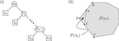
Figure 8: (i) Structure of the tree for the lower-bound construction. (ii) Illustration for the proof of Lemma 4.

The structure of $\mathcal{T}$ is depicted in Fig. 8(i). The tree $\mathcal{T}$ has $h+1$ nodes $\nu_{0},\ldots,\nu_{h}$ that form a path, and $h$ other (leaf) nodes $\lambda_{1},\ldots,\lambda_{h}$ branching off the path. The idea will be to choose the weights of the leaves very small, so that the only way to give the region $P(\lambda_{i})$ the required area, is to cut off a small triangle from $P(\nu_{i})$. Then we will argue that one of these triangles must have a small angle.

To make this idea precise we define

$$x_{i}:=\begin{cases}1&\mbox{if $i=0$,}\\ x_{i-1}/(2\sqrt{h})&\mbox{if $0<i\leq h$,}\end{cases}$$

and we set $w(\lambda_{i}):=x_{i-1}^{2}/(4h)$ for $1\leq i\leq h$. Note that defining the weights for $\lambda_{1},\ldots,\lambda_{h}$ implicitly defines the weights for $\nu_{1},\ldots,\nu_{h}$ as well.

Lemma 4.

If each region created in a polygonal partition for $\mathcal{T}$ has aspect ratio at most $h$, then we have for $0\leq i\leq h$,

1. $P(\lambda_{i-1})$ is a triangle (if $\lambda_{i-1}$ exists, that is, if $i\neq 0$);

2. $P(\nu_{i})$ has $i+4$ sides, each of length at least $x_{i}$.

Proof.

We will prove the lemma by induction on $i$. For $i=0$ the lemma is obviously true, since $P(\nu_{0})$ is the unit square.

Now let $i>0$. By the induction hypothesis, each side of $P(\nu_{i-1})$ has length at least $x_{i-1}$. If $P(\lambda_{i})$ fully contained an edge of $P(\nu_{i-1})$, its diameter would therefore be more than $x_{i-1}$. But then its aspect ratio would be

$$\frac{\operatorname{diam}(P(\lambda_{i}))^{2}}{\operatorname{area}(P(\lambda_{i}))}\geq\frac{x_{i-1}^{2}}{w(\lambda_{i})}=\frac{x_{i-1}^{2}}{x_{i-1}^{2}/4h}=4h,$$

which contradicts the assumptions. Hence, $P(\lambda_{i})$ is a triangle, as claimed. It also follows that $P(\nu_{i})$ has $i+4$ sides. It remains to show that these sides have length at least $x_{i}$.

Let $st$ be the segment that cuts $P(\nu_{i-1})$ into $P(\nu_{i})$ and $P(\lambda_{i})$, let $p$ be the corner of $P(\nu_{i-1})$ that is cut off, and let $q$ and $r$ be the corners of $P(\nu_{i-1})$ adjacent to $p$—see Fig. 8(ii). All sides of $P(\nu_{i})$ except $qs$, $st$, and $tr$ have length at least $x_{i-1}$ so they definitely have length at least $x_{i}$.

It is easy to see that the angles of any polygon $P(\nu_{j})$ are at least $\pi/2$—indeed, when a corner is cut off from some $P(\nu_{j})$, the two new angles appearing in $P(\nu_{j+1})$ are larger than the angle at the corner that is cut off. Hence, $st$ is the longest edge of the triangle $pst=P(\lambda_{i})$, and we have

$$|st|\geq\sqrt{\operatorname{area}(P(\lambda_{i}))}=\sqrt{w(\lambda_{i})}=\sqrt{\frac{x_{i-1}^{2}}{4h}}=\frac{x_{i-1}}{2\sqrt{h}}=x_{i}.$$

Next we show that $qs$ has length at least $x_{i}$; the argument for $tr$ is similar. Note that $|ps|\leq\sqrt{h\cdot w(\lambda_{i})}$, otherwise $P(\lambda_{i})$’s aspect ratio would be larger than $h$. Hence, we have

$$|qs| =|pq|-|ps|$$

$$\geq x_{i-1}-|ps|\qquad\mbox{(induction hypothesis)}$$

$$\geq x_{i-1}-\sqrt{h\cdot w(\lambda_{i})}$$

$$=x_{i-1}-\sqrt{h\cdot\frac{x_{i-1}^{2}}{4h}}$$

$$=\frac{x_{i-1}}{2}$$

$$\geq x_{i}.$$

∎

Next we show that one of the triangles $P(\lambda_{i})$ must have large aspect ratio.

Lemma 5.

If each region created in a polygonal partition for $\mathcal{T}$ has aspect ratio at most $h$, then there is a region $P(\lambda_{i})$ where one of whose interior angles is at most $2\pi/(h+4)$.

Proof.

By the previous lemma, the region $P(\nu_{h})$ has $h+4$ sides. The sum of the interior angles of a $(h+4)$-gon is exactly $(h+2)\cdot 2\pi$, so one of the interior angles of $P(\nu_{h})$ must be at least

$$\frac{(h+2)\cdot 2\pi}{h+4}=2\pi-\frac{4\pi}{h+4}.$$

If the two edges meeting at some corner $p$ of $P(\nu_{h})$ make an angle of at least $2\pi-4\pi/(h+4)$ in $P(\nu_{h})$, then they must make an angle of at most $4\pi/(h+4)$ in a region $P(\lambda_{i})$ adjacent to $p$. ∎

Theorem 3.

For any $h$, there is a weighted tree $\mathcal{T}$ of height $h$ such that any polygonal partition for $\mathcal{T}$ has aspect ratio $\Omega(h)$.

Proof.

Consider the tree $\mathcal{T}$ described above. Assume the aspect ratio of the polygonal partition for $\mathcal{T}$ is less than $h$—otherwise we are done. Then by Lemma 5 there is a region with interior angle $4\pi/(h+4)$. By Observation 1 this region has aspect ratio at least $(h+4)/2\pi=\Omega(h)$. ∎

6 Partitions with slack

Recall that a rectangular partition is a polygonal partition in which all polygons are rectangles. We show that if we allow a small distortion of the areas of the rectangles, then there exists a rectangular partition of small aspect ratio. This result can also be obtained for partitions of a hypercube in ${\mathbb{R}}^{d}$. We now define more precisely which type of distortion we allow.

Let $\mathcal{T}$ be a properly weighted tree. A rectangular partition with $\varepsilon$-slack in ${\mathbb{R}}^{d}$ for $\mathcal{T}$ assigns a $d$-dimensional hyperrectangle $R(\nu)$ to each node $\nu\in\mathcal{T}$ such that

• the hyperrectangle $R(\operatorname{root}(\mathcal{T}))$ is the unit hypercube in ${\mathbb{R}}^{d}$;

• for any two nodes $\nu,\mu$ such that $\mu$ is a child of $\nu$ we have

  $$(1-\varepsilon)\cdot\frac{\mathop{\rm vol}(R(\mu))}{w(\mu)}\leq\frac{\mathop{\rm vol}(R(\nu))}{w(\nu)}\leq\frac{\mathop{\rm vol}(R(\mu))}{w(\mu)}.$$

• for any node $\nu$, the hyperrectangles assigned to the children of $\nu$ have pairwise disjoint interiors and are contained in $R(\nu)$.

Observe that as we go down the tree $\mathcal{T}$, the volumes of the hyperrectangles can start to deviate more and more from their weights. However, the relative volumes of the hyperrectangles of the children of a node $\nu$ stay roughly the same and together they still cover $R(\nu)$ almost entirely.

For convenience, we will work with the rectangular aspect ratio of a $d$-dimensional hyperrectangle rather than using the aspect-ratio definition given earlier. The rectangular aspect ratio $\operatorname{asp}_{\rm rect}(R)$ of hyperrectangle $R$ with side lengths $s_{1},s_{2},\ldots,s_{d}$ is defined as $\operatorname{asp}_{\rm rect}(R):=\frac{\max_{i}s_{i}}{\min_{i}s_{i}}$. It can easily be shown that for 2-dimensional rectangles, the aspect ratio and the rectangular aspect ratio are within a constant factor. We define the rectangular aspect ratio of a rectangular partition as the maximum rectangular aspect ratio of any of the hyperrectangles in the partition.

Our algorithm to construct a rectangular partition always cuts perpendicular to the longest side of a hyperrectangle $R(\nu)$. Since we can shrink each of the hyperrectangles of the children of $\nu$ by a factor $1-\varepsilon$, we have some extra space to keep the aspect ratios under control. We will prove that this means that the longest-side-first strategy can ensure a rectangular aspect ratio of $1/\varepsilon$. The basic tool is the following lemma.

Lemma 6.

Let $0<\varepsilon<1/3$, and let $R$ be a hyperrectangle with $\operatorname{asp}_{\rm rect}(R)\leq 1/\varepsilon$. Let $S=\{w_{1},\ldots,w_{k}\}$ be a set of weights with $\sum_{i=1}^{k}w_{i}=(1-\varepsilon)\cdot\mathop{\rm vol}(R)$. Then there exists a set $\{R_{1},\ldots,R_{k}\}$ of pairwise disjoint hyperrectangles, each contained in $R$, such that for all $1\leq i\leq k$ we have $\mathop{\rm vol}(R_{i})=w_{i}$ and $\operatorname{asp}_{\rm rect}(R_{i})\leq 1/\varepsilon$.

Proof.

We will prove this by induction on $k$. The case $k=1$ is trivial, so now assume $k>1$. For a subset $S^{\prime}\subset S$, we define $w(S^{\prime}):=\sum_{w_{i}\in S^{\prime}}w_{i}$. Assume without loss of generality that $w_{1}=\max_{i}w_{i}$. There are two cases.

• If $w_{1}\leq(1-\varepsilon)\cdot w(S)$, then we can split $S$ into subsets $S^{\prime}$ and $S^{\prime\prime}$ such that $w(S^{\prime})\geq\varepsilon\cdot w(S)$ and $w(S^{\prime\prime})\geq\varepsilon\cdot w(S)$. Indeed, if $i^{*}$ is the minimum index such that $\sum_{i=1}^{i^{*}}w_{i}\geq\varepsilon\cdot w(S)$, then $\sum_{i=1}^{i^{*}}w_{i}\leq(1-\varepsilon)\cdot w(S)$ since $\varepsilon<1/3$. Hence, setting $S^{\prime}=\{w_{1},\ldots,w_{i^{*}}\}$ satisfies the condition.

  We now cut $R$ perpendicular to its longest side into hyperrectangles $R^{\prime}$ and $R^{\prime\prime}$ such that

  $$\mathop{\rm vol}(R^{\prime})=\mathop{\rm vol}(R)\cdot\frac{w(S^{\prime})}{w(S)}\ \ \mbox{ and }\ \ \mathop{\rm vol}(R^{\prime\prime})=\mathop{\rm vol}(R)\cdot\frac{w(S^{\prime\prime})}{w(S)}.$$

  Note that this implies that

  $$w(S^{\prime})=\frac{w(S)}{\mathop{\rm vol}(R)}\cdot\mathop{\rm vol}(R^{\prime})=(1-\varepsilon)\cdot\mathop{\rm vol}(R^{\prime}).$$

  Since $w(S^{\prime})\geq\varepsilon\cdot w(S)$ and the cut is perpendicular to the longest side, we have $\operatorname{asp}_{\rm rect}(R^{\prime})\leq 1/\varepsilon$. Hence, by induction there exists a set of pairwise disjoint hyperrectangles, each contained in $R^{\prime}$, whose volumes are the weights in $S^{\prime}$ and whose aspect ratios are at most $1/\varepsilon$. Similarly, there is a collection of suitable hyperrectangles contained in $R^{\prime\prime}$ for the weights in $S^{\prime\prime}$. Hence, we have found a set of hyperrectangles for $S$ satisfying all the conditions.

• If $w_{1}>(1-\varepsilon)\cdot w(S)$ we split $R$ into $R_{1}$ and $R^{\prime}$ by cutting perpendicular to the longest side, such that $\mathop{\rm vol}(R_{1})=w_{1}$. Since

  $$w_{1}>(1-\varepsilon)\cdot w(S)=(1-\varepsilon)^{2}\cdot\mathop{\rm vol}(R)>\varepsilon\cdot\mathop{\rm vol}(R),$$

  we have $\operatorname{asp}_{\rm rect}(R_{1})\leq 1/\varepsilon$. Furthermore, since $w(S)=(1-\varepsilon)\cdot\mathop{\rm vol}(R)$ we certainly have $w_{1}<(1-\varepsilon)\cdot\mathop{\rm vol}(R)$, and so

  $$\mathop{\rm vol}(R^{\prime})=\mathop{\rm vol}(R)-w_{1}>\varepsilon\cdot\mathop{\rm vol}(R).$$

  This implies that $\operatorname{asp}_{\rm rect}(R^{\prime})\leq 1/\varepsilon$. Finally, we note that

  $$\frac{w(S\setminus\{w_{1}\})}{\mathop{\rm vol}(R^{\prime})}=\frac{w(S)-w_{1}}{\mathop{\rm vol}(R)-w_{1}}<\frac{w(S)}{\mathop{\rm vol}(R)}=1-\varepsilon.$$

  Hence, we can slightly shrink $R^{\prime}$ such that $w(S\setminus\{w_{1}\})=(1-\varepsilon)\cdot\mathop{\rm vol}(R^{\prime})$, which means we can apply the induction hypothesis to obtain a suitable set of hyperrectangles for the weights in $S\setminus\{w_{1}\}$ inside $R^{\prime}$. Together with the hyperrectangle $R_{1}$ for $w_{1}$, this gives us a collection of hyperrectangles for the weights in $S$ satisfying all the conditions.

∎

We can now prove our final result on partitions with slack.

Theorem 4.

Let $0<\epsilon<1/3$, and let $d\geq 2$. Let $\mathcal{T}$ be a properly weighted tree. Then there exists a rectangular partition with $\varepsilon$-slack in ${\mathbb{R}}^{d}$ for $\mathcal{T}$ whose aspect ratio is at most $1/\varepsilon$.

Proof.

We construct the rectangular partition recursively, as follows. We start at the root of $\mathcal{T}$, where we set $R(\operatorname{root}(\mathcal{T}))$ to the unit hypercube. Note that the rectangular aspect ratio of a hypercube is 1. Now, given a hyperrectangle $R(\nu)$ of an internal node $\nu$ such that the rectangular aspect ratio is at most $1/\varepsilon$, we will construct hyperrectangles for the children of $\nu$ of the required aspect ratio. To this end, for any child $\mu$ of $\nu$ we define

$$w^{*}(\mu):=(1-\varepsilon)\cdot w(\mu)\cdot\frac{\mathop{\rm vol}(R(\nu))}{w(\nu)}.$$

Observe that since $\sum_{\mu}w(\mu)=w(\nu)$, we have

$$\sum_{\mu}w^{*}(\mu)=(1-\varepsilon)\cdot\mathop{\rm vol}(R(\nu)).$$

Hence, we can apply Lemma 6 with $S=\{w^{*}(\mu):\mbox{ $\mu$ is a child of $\nu$}\}$ to partition $R(\nu)$ into pairwise disjoint hyperrectangles $R_{\mu}$, each contained in $R(\nu)$ and of aspect ratio at most $1/\varepsilon$. The volume of each $R(\mu)$ will be $w^{*}(\mu)$, which is in the allowed range. Finally, we recurse on each non-leaf child. After we the recursive process has finished, we have the desired partition. ∎

7 Embedding ultrametrics into $\mathbb{R}^{d}$

Before we describe our algorithm for embedding ultrametrics into $\mathbb{R}^{d}$, we define $\alpha$-hierarchical well separated trees, or $\alpha$-HSTs for short, introduced by Bartal [4]. Let $\alpha>1$ be a parameter. An $\alpha$-HST is a rooted tree $\mathcal{T}$ with all leaves on the same level, where each node $\nu$ has an associated label $l(\nu)$ such that for any node $\nu$ with parent $\mu$ we have $l(\mu)=\alpha\cdot l(\nu)$. The metric space that corresponds to the HST $\mathcal{T}$ is defined on the leaves of $\mathcal{T}$, and the distance between any two leaves in $\mathcal{T}$ is equal to the label of the their lowest common ancestor.

Let $M=(X,D)$ be the given ultrametric. After scaling $M$, we can assume that the minimum distance is 1 and the diameter is $\Delta$. For any $\alpha>1$, we can embed $M$ into an $\alpha$-HST, with distortion $\alpha$ [5]. Given $M$, we initially compute an embedding of $M$ into a $2$-HST $\mathcal{T}$ with distortion 2. Let $M_{\mathcal{T}}=(X,D_{\mathcal{T}})$ be the metric space corresponding to $\mathcal{T}$. Any embedding of $M_{\mathcal{T}}$ into ${\mathbb{R}}^{d}$ with distortion $c^{\prime}$, yields an embedding of $M$ into $\mathbb{R}^{d}$ with distortion $O(c^{\prime})$. It therefore suffices to embed of $M_{\mathcal{T}}$ into ${\mathbb{R}}^{d}$. With a slight abuse of notation we will from now on denote the leaf of $\mathcal{T}$ corresponding to a point $x\in X$ simply by $x$.

A lower bound.

To prove the approximation ratio of our embedding algorithm, we need a lower bound on the optimal distortion. We will use the lower bound proved by Bădoiu et al. [9], which we describe next.

Consider an embedding $\phi$ of $M_{\mathcal{T}}$ into $\mathbb{R}^{d}$. Assume without loss of generality that $\phi$ is non-contracting, that is, $\phi$ does not make any distances smaller. For each node $\nu\in\mathcal{T}$ we define a set $A_{\nu}\subset\mathbb{R}^{d}$ as follows. Let $B_{d}(r)$ denote the ball in ${\mathbb{R}}^{d}$ centered at the origin and of radius $r$. For a leaf $\nu$ of $\mathcal{T}$, let $A_{\nu}$ be equal to the ball $B_{d}(\frac{1}{2})$ translated so that its center is $\phi(\nu)$. For a non-leaf node $\nu$ with children $\mu_{1},\ldots,\mu_{k}$, let $A_{\nu}$ be the Minkowski sum of $\bigcup_{i=1}^{k}A_{\mu_{i}}$ with $B_{d}(l(\nu))$. By the non-contraction of $\phi$ it follows that for each pair of nodes $\nu,\nu^{\prime}$ that are on the same level of $\mathcal{T}$, the regions $A_{\nu}$ and $A_{\nu^{\prime}}$ have disjoint interiors—see Figure 9 for an example. Intuitively, the volume $A_{\nu}$ is necessary to embed all the points corresponding to the leaves below $\nu$ such that the embedding is non-contracting. This in turn can be used via an isoperimetric argument to obtain a lower bound on the maximum distance (and, hence, distortion) between the images of these leaves.

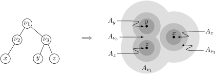
Figure 9: The sets $A_{\nu}$ for a non-contracting embedding of an HST.

We cannot compute $A_{\nu}$ exactly, however, since we do not know the embedding. Hence, following Bădoiu et al. [9] we define for each $\nu\in\mathcal{T}$ a value $A^{*}(\nu)$ that estimates the volume of $A_{\nu}$. Intuitively, the estimate on $A_{\nu}$ is derived by the Brunn-Minkowski inequality. More precisely, we define $A^{*}(\nu)$ as follows.

$$A^{*}(\nu)=\begin{cases}\mathop{\rm vol}\left(B_{d}(\frac{1}{2})\right)&\mbox{if $\nu$ is a leaf,}\\ \sum_{\mbox{$\mu$ is a child of $\nu$}}\left(A^{*}(\mu)^{1/d}+\mathop{\rm vol}\left(B_{d}\left(\frac{l(\nu)}{4}\right)\right)^{1/d}\right)^{d}&\mbox{otherwise.}\end{cases}$$

The estimate $A^{*}(\nu)$ can be used to obtain a lower bound on the distortion, as made precise in the next lemma. For any $V>0$, let $r_{d}(V)$ be the radius of a $d$-dimensional ball with volume $V$; thus we have

$$r_{d}(V)=\left(\frac{V\cdot\Gamma(1+d/2)}{\pi^{d/2}}\right)^{1/d}=\Theta\left(\sqrt{d}\cdot V^{1/d}\right),$$

where $\Gamma(z)=\int_{0}^{\infty}t^{z-1}e^{-t}dt$.

Lemma 7 ([9], Corollary 1).

Let opt denote the distortion of an optimal embedding of $M_{\mathcal{T}}$ into $\mathbb{R}^{d}$. Then

$$\mbox{{\sc opt}}\geq\max_{\mbox{\rm\small$\nu$ is internal node of $\mathcal{T}$}}\frac{r_{d}(A^{*}(\nu))}{l(\nu)}-1.$$

The algorithm.

We are now ready to describe the embedding $f$ of $M_{\mathcal{T}}$ into $\mathbb{R}^{d}$. The intuition behind our algorithm is as follows. The lower bound given by Lemma 7 implies that an embedding is nearly-optimal if it results in sets $A_{\nu}$ with small aspect ratio. Our approach, however, is essentially reversed. We first compute a hyperrectangular partition of $\mathbb{R}^{d}$ into hyperrectangles with small aspect ratio. The hyperrectangle computed for the leaves in $\mathcal{T}$ will roughly correspond to the balls around the embedded points $x\in X$, so given the partition we will be able to obtain the embedding by placing $f(x)$ at the center of the hyperrectangle computed for $x$. The weights we use for the nodes of $\mathcal{T}$ will be the values $A^{*}(\nu)$, which using Lemma 7 can then be used to bound the distortion.

More precisely, the algorithm works as follows.

1. Compute for each node $\nu\in\mathcal{T}$ the value $A^{*}_{\nu}$.

2. Compute a hyperrectangular partition with slack $\varepsilon:=\min(\frac{1}{3},\frac{1}{\log\Delta})$ for $\mathcal{T}$, where $A^{*}_{\nu}$ is used as the weight of a node $\nu$. Note that $\mathcal{T}$ is not properly weighted: the weight of $\operatorname{root}(\mathcal{T})$ will be greater than 1 and the weight of an internal node $\nu$ is larger than the sum of the weights of its children. However, we can still apply Theorem 4. Indeed, by scaling the weights appropriately we can ensure that the root has weight 1, and the fact that the weight of an internal node $\nu$ is larger than the sum of the weights of its children only makes it easier to obtain a small aspect ratio. Thus we can compute a hyperrectangular partition for $\mathcal{T}$ whose rectangular aspect ratio is at most $\log\Delta$.

3. Let $P(\nu)$ denote the hyperrectangle computed for node $\nu\in\mathcal{T}$ in Step 2. We slightly modify the hyperrectangles $P(\nu)$, as follows. Starting from the root of $\mathcal{T}$, we traverse all the nodes of $\mathcal{T}$. When we visit an internal node $\nu$, we shrink all hyperrectangles of the nodes in the subtree rooted at $\nu$ by a factor of $1-1/\log\Delta$, with the center of the (current) hyperrectangle $P^{\prime}(\nu)$ of $\nu$ being the fixed point in the transformation. Note that $P^{\prime}(\nu)$ itself is not shrunk. Thus the shrinking step moves the hyperrectangles contained inside $P^{\prime}(\nu)$ away from its boundary and towards its center, thus preventing points in different subtrees to get too close to each other.

4. Let $P^{\prime}(\nu)$ denote the hyperrectangle computed in Step 3. Then we define the embedding $f(x)$ of a point $x\in X$ to be the center of the hyperrectangle $P^{\prime}(x)$.

It remains to bound the distortion of $f$. We will need the following observation, which bounds the diameter of a hyperrectangle in terms of its volume and aspect ratio.

Observation 2.

Let $P$ be a hyperrectangle in ${\mathbb{R}}^{d}$ with aspect ratio at most $\alpha$. Then, assuming $\alpha\geq\sqrt{d-1}$,

$$\operatorname{diam}(P)\leq\alpha\sqrt{2}\cdot\mathop{\rm vol}(P)^{1/d}.$$

From now on we assume that $\log\Delta\geq\sqrt{d-1}$.

Lemma 8.

The expansion of $f$ is $O\left(\frac{1}{\sqrt{d}}\cdot\log{\Delta}\cdot\mbox{{\sc opt}}\right)$.

Proof.

Consider points $x,y\in X$. Let $\nu$ be the lowest common ancestor of $x$ and $y$ in $\mathcal{T}$. We have $D_{\mathcal{T}}(x,y)=l(\nu)$. Both $f(x)$ and $f(y)$ are contained in $P^{\prime}(\nu)$, which in turn is contained in $P(\nu)$. Hence, $\operatorname{diam}(P(\nu))$ gives an upper bound on $|xy|$. Note that $\operatorname{asp}_{\rm rect}(P(\nu))\leq\log\Delta$ and that $\mathop{\rm vol}(P(\nu))\leq A^{*}_{\nu}$. (We do not necessarily have $\mathop{\rm vol}(P(\nu))=A^{*}_{\nu}$ because of the slack in the partition.) Hence,

$$|xy| \leq\textstyle\operatorname{diam}(P(\nu))$$

$$\leq\textstyle\log\Delta\cdot\sqrt{2}\cdot\mathop{\rm vol}(P(\nu))^{1/d}$$

$$\leq\textstyle\log\Delta\cdot\sqrt{2}\cdot\left(A^{*}_{\nu}\right)^{1/d}$$

$$=\textstyle O\left(\log\Delta\cdot r_{d}(A^{*}_{\nu})\cdot\frac{1}{\sqrt{d}}\right)$$

$$=\textstyle O\left(\log\Delta\cdot(\mbox{{\sc opt}}+1)\cdot l(\nu)\cdot\frac{1}{\sqrt{d}}\right)$$

$$=\textstyle O\left(\log\Delta\cdot\mbox{{\sc opt}}\cdot D_{\mathcal{T}}(x,y)\cdot\frac{1}{\sqrt{d}}\right),$$

where the second-to-last transition follows from Lemma 7. This shows that the expansion is $O(\log{\Delta}\cdot\mbox{{\sc opt}}\cdot\frac{1}{\sqrt{d}})$. ∎

Lemma 9.

The contraction of $f$ is $O\left(\sqrt{d}\cdot\log^{2}{\Delta}\right)$.

Proof.

Since $\mathcal{T}$ is a 2-HST, we have $\Delta=l(\operatorname{root}(\mathcal{T}))=2^{\operatorname{height}(\mathcal{T})}$. Hence, $\operatorname{height}(\mathcal{T})=\log\Delta$. It follows that for each node $\nu\in\mathcal{T}$,

$$\mathop{\rm vol}(P^{\prime}(\nu)) =\Omega\left(\left(1-\frac{1}{\log\Delta}\right)^{\log\Delta}\cdot\mathop{\rm vol}(P(\nu))\right)=\Omega\left(\mathop{\rm vol}(P(\nu))\right)$$

$$=\Omega\left(\left(1-\frac{1}{\log\Delta}\right)^{\log\Delta}\cdot A^{*}_{\nu}\right)=\Omega\left(A^{*}_{\nu}\right).$$

Consider points $x,y\in X$, and let $\nu$ be the lowest common ancestor of $x$ and $y$ in $\mathcal{T}$. We will consider the following two cases for $\nu$:

• Case 1: $\nu$ is the parent of $x$ and $y$ in $\mathcal{T}$.
  Since the minimum distance in $M_{\mathcal{T}}$ is 1, it follows that $D_{\mathcal{T}}(x,y)=1$. By construction, $f(x)$ is the center of $P^{\prime}(x)$. Let $t$ be the distance between $f(x)$ and $\operatorname{\partial}P^{\prime}(x)$. Since $\operatorname{asp}_{\rm rect}(P^{\prime}(x))\leq 1/\varepsilon$, we have

  $$t\geq\varepsilon\cdot\mathop{\rm vol}(P^{\prime}(x))^{1/d}=\Omega\left(\varepsilon\cdot(A^{*}_{x})^{1/d}\right)=\Omega\left(\varepsilon\cdot\frac{1}{\sqrt{d}}\right)=\Omega\left(\frac{1}{\sqrt{d}\log\Delta}\right).$$

  Thus, $|f(x)f(y)|\geq t=\Omega\left(\frac{D(x,y)}{\sqrt{d}\log\Delta}\right)$.

• Case 2: $\nu$ is not the parent of $x$ and $y$ in $\mathcal{T}$.
  Let $\mu$ be the child of $\nu$ that lies on the path from $\nu$ to $x$. Let $t$ be the distance between $x$ and $\operatorname{\partial}P^{\prime}(\mu)$. Because of the shrinking performed in Step 3, we know that $t\geq(1/\log\Delta)\cdot(s/2)$, where $s$ is the length of the shortest edge of $P^{\prime}(\mu)$. Since $\operatorname{asp}_{\rm rect}(P^{\prime}(\mu))\leq 1/\varepsilon$, we have $s\geq\varepsilon^{1-1/d}\cdot\mathop{\rm vol}(P^{\prime}(\mu))^{1/d}$. Hence,

  $$t \geq\textstyle\frac{1}{\log\Delta}\cdot\frac{s}{2}$$

  $$=\textstyle\Omega\left(\frac{\varepsilon^{1-1/d}}{\log\Delta}\cdot\mathop{\rm vol}(P^{\prime}(\mu))^{1/d}\right)$$

  $$=\textstyle\Omega\left(\frac{\varepsilon^{1-1/d}}{\log\Delta}\cdot(A^{*}_{\mu})^{1/d}\right)$$

  $$=\textstyle\Omega\left(\frac{1}{\log^{2}\Delta}\cdot(A^{*}_{\mu})^{1/d}\right)$$

  $$=\textstyle\Omega\left(\frac{1}{\log^{2}\Delta}\cdot l(\mu)\cdot\frac{1}{\sqrt{d}}\right)$$

  $$=\textstyle\Omega\left(\frac{D(x,y)}{\sqrt{d}\log^{2}\Delta}\right).$$

∎

Combining Lemmas 8 and 9 we obtain the main result of the section.

Theorem 5.

For any fixed $d\geq 2$, there exists a polynomial-time, $O\left(\sqrt{d}\cdot\log^{3}\Delta\right)$-approximation algorithm for the problem of embedding ultrametrics into $\mathbb{R}^{d}$ with minimum distortion.

We remark that the running time of the above algorithm depends on the way the input is given. If the ultrametric is given as a matrix of pairwise distances, then one needs to first compute a tree representation, with the points being the leaves of the tree. For an $n$-point ultrametric, this task takes at least $\Omega(n^{2})$ time. Given such a tree representation, for any fixed dimension $d$, it is fairly easy to implement our algorithm in roughly quadratic time. It is an interesting open problem to obtain an algorithm with near-linear running time.

As a final comment, note that while the approximation factor is relatively small (for instance, for $\Delta=n^{O(1)}$ and constant $d$, it becomes $O(\log^{3}n)$), the distortion itself can be much larger. For example, embedding the uniform metric on $n$ vertices (which is an ultrametric as well) into $\mathbb{R}^{d}$ requires distortion $\Omega(n^{1/d})$ for constant $d$.

References

- [1] M. Balzer and O. Deussen. Voronoi treemaps. In INFOVIS, page 7, 2005.
- [2] M. Balzer, O. Deussen, and C. Lewerentz. Voronoi treemaps for the visualization of software metrics. In SOFTVIS, pages 165–172, 2005.
- [3] Y. Bartal. Probabilistic approximation of metric spaces and its algorithmic applications. In 37th Annual Symposium on Foundations of Computer Science (Burlington, VT, 1996), pages 184–193. IEEE Comput. Soc. Press, Los Alamitos, CA, 1996.
- [4] Y. Bartal. Probabilistic approximation of metric spaces and its algorithmic applications. Annual Symposium on Foundations of Computer Science, 1996.
- [5] Y. Bartal and M. Mendel. Dimension reduction for ultrametrics. In SODA ’04: Proceedings of the fifteenth annual ACM-SIAM symposium on Discrete algorithms, pages 664–665, Philadelphia, PA, USA, 2004. Society for Industrial and Applied Mathematics.
- [6] B. B. Bederson, B. Shneiderman, and M. Wattenberg. Ordered and quantum treemaps: Making effective use of 2d space to display hierarchies. ACM Trans. Graph., 21(4):833–854, 2002.
- [7] J. Bourgain. On lipschitz embedding of finite metric spaces into hilbert space. Isreal Journal of Mathematics, 52:46–52, 1985.
- [8] D. M. Bruls, C. Huizing, and J. J. van Wijk. Squarified treemaps. In W. de Leeuw, R. van Liere (eds.), Data Visualization 2000, Proceedings of the joint Eurographics and IEEE TCVG Symposium on Visualization, pages 33–42. Springer, 2000.
- [9] M. Bădoiu, J. Chuzhoy, P. Indyk, and A. Sidiropoulos. Embedding ultrametrics into low-dimensional spaces. In Proceedings of the 22nd ACM Symposium on Computational Geometry, 2006.
- [10] M. de Berg, B. Speckmann, and V. van der Weele. Treemaps with bounded aspect ratio. CoRR, abs/1012.1749, 2010.
- [11] M. de Berg, A. F. van der Stappen, J. Vleugels, and M. J. Katz. Realistic input models for geometric algorithms. Algorithmica, 34(1):81–97, 2002.
- [12] P. Indyk. Tutorial: Algorithmic applications of low-distortion geometric embeddings. Annual Symposium on Foundations of Computer Science, 2001.
- [13] L. Jin and D. C. Banks. Tennisviewer: A browser for competition trees. IEEE Computer Graphics and Applications, 17(4):63–65, 1997.
- [14] B. Johnson and B. Shneiderman. Tree-maps: a space-filling approach to the visualization of hierarchical information structures. In Proc., IEEE Conference on Visualization, pages 284–291, 1991.
- [15] W.-A. Jungmeister and D. Turo. Adapting treemaps to stock portfolio visualization. Technical Report UMCP-CSD CS-TR-2996, College Park, Maryland 20742, U.S.A., 1992.
- [16] J. Matoušek. Bi-Lipschitz embeddings into low-dimensional Euclidean spaces. Comment. Math. Univ. Carolinae, 31:589–600, 1990.
- [17] J. Matoušek and A. Sidiropoulos. Inapproximability for metric embeddings into . In 49th IEEE Symposium on Foundations of Computer Science, 2008.
- [18] K. Onak and A. Sidiropoulos. Circular partitions with applications to visualization and embeddings. In Proceedings of the 24nd ACM Symposium on Computational Geometry, pages 28–37, 2008.
- [19] F. P. Preparata and M. I. Shamos. Computational Geometry: An Introduction. Springer-Verlag, New York, NY, 1985.
- [20] B. Shneiderman. Treemaps for space-constrained visualization of hierarchies. Available at http://www.cs.umd.edu/hcil/treemap-history/index.shtml.
- [21] B. Shneiderman. Tree visualization with tree-maps: 2-d space-filling approach. ACM Trans. Graph., 11(1):92–99, 1992.
- [22] B. Shneiderman and M. Wattenberg. Ordered treemap layouts. In IEEE Symposium on Information Visualization, INFOVIS ’01, pages 73–78, 2001.
- [23] D. Turo and B. Johnson. Improving the visualization of hierarchies with treemaps: Design issues and experimentation. IEEE Visualization, pages 124–131, 1992.
- [24] R. Vliegen, J. J. van Wijk, and E.-J. van der Linden. Visualizing business data with generalized treemaps. IEEE Transactions on Visualization and Computer Graphics, 12(5):789–796, 2006.
-
[25]
S. Wan.
Blog treemap visualizer
(http://www.samuelwan.com/information/archives/000159.html). - [26] M. Weskamp. Newsmap. http://marumushi.com/apps/newsmap/newsmap.cfm.
- [27] K. Wetzel. Using Circular Treemaps to visualize disk usage. Available at http://lip.sourceforge.net/ctreemap.html.