Characterizing the Variability of Stars with Early-Release Kepler Data

Abstract

We present a variability analysis of the early-release first quarter of data publicly released by the Kepler project. Using the stellar parameters from the Kepler Input Catalog, we have separated the sample into 129,000 dwarfs and 17,000 giants, and further sub-divided the luminosity classes into temperature bins corresponding approximately to the spectral classes A, F, G, K, and M. Utilizing the inherent sampling and time baseline of the public dataset (30 minute sampling and 33.5 day baseline), we have explored the variability of the stellar sample. The overall variability rate of the dwarfs is 25% for the entire sample, but can reach 100% for the brightest groups of stars in the sample. G-dwarfs are found to be the most stable with a dispersion floor of $\sigma\sim 0.04$ mmag. At the precision of Kepler, $>95$% of the giant stars are variable with a noise floor of $\sim 0.1$ mmag, 0.3 mmag, and 10 mmag for the G-giants, K-giants, and M-giants, respectively. The photometric dispersion of the giants is consistent with acoustic variations of the photosphere; the photometrically-derived predicted radial velocity distribution for the K-giants is in agreement with the measured radial velocity distribution. We have also briefly explored the variability fraction as a function of dataset baseline (1 - 33 days), at the native 30-minute sampling of the public Kepler data. To within the limitations of the data, we find that the overall variability fractions increase as the dataset baseline is increased from 1 day to 33 days, in particular for the most variable stars. The lower mass M-dwarf, K-dwarf, G-dwarf stars increase their variability more significantly than the higher mass F-dwarf and A-dwarf stars as the time-baseline is increased, indicating that the variability of the lower mass stars is mostly characterized by timescales of weeks while the variability of the higher mass stars is mostly characterized by timescales of days. A study of the distribution of the variability as a function of galactic latitude suggests sources closer to the galactic plane are more variable. This may be the result of sampling differing populations (i.e., ages) as a function of latitude or may be the result of higher background contamination that is inflating the variability fractions at lower latitudes. A comparison of the M dwarf statistics to the variability of 29 known bright M dwarfs indicates that the M dwarfs are primarily variable on timescales of weeks or longer presumably dominated by spots and binarity. But on shorter timescales of hours which are relevant for planetary transit detection, the stars are significantly less variable, with $\sim 80$% having 12-hour dispersions of 0.5 mmag or less.

1. Introduction

Stars have been known for a long time to vary in brightness, and photometric studies over the past centuries have revealed many classes of stars exhibiting a variety of variability (Pickering, 1881). With interest in stellar variability growing tremendously in the last decade as ground-based and space-based surveys for exoplanets have gained momentum, understanding the stellar photometric variability is even more crucial.

Sources of stellar variability include pulsations, binarity, rotation, and activity (e.g., Eyer & Mowlavi, 2008). Having a large sample of uniformly observed stars is vital in the categorization and characterization of the variability which can inform us about the stars themselves, their companions and companion rates, and their evolution. The fractions of stars that are found to be variable is dependent upon the sample of stars studied, the precision of the survey, the range of magnitudes over which the precision is matched, and the time duration of the survey (e.g., Eyer & Mowlavi, 2008; Howell, 2008). For example, Hipparcos (with mmag precision and a completeness limit near V=8 mag) found 10% of the stars in the sample to be variable (Eyer & Grenon, 1997; Eyer & Mowlavi, 2008), but the variability fraction depended upon both the stellar brightness and the stellar type. Similar population and precision dependent results have been found by survey programs intended for other purposes such as microlensing studies and transit surveys (e.g.,OGLE (Wozniak & Szymanski, 1998), HATNet (Hartman et al., 2004), and WASP0 (Kane et al., 2005)) as well as from general variability programs (e.g., BSVS (Everett et al., 2002), FSVS (Huber, Everett, & Howell, 2006), and ASAS (Pojmanski, 2002)).

As the surveys have become more sensitive, the fraction of stars observed to vary has been found to increase in a form which can be described by a power-law distribution directly proportional to the quality of the photometric precision (Howell, 2008). This is a result of the current “best” survey precisions, time samplings, and survey durations probing ever deeper into the variability of stars but generally not reaching the astrophysical variability floor.

Spaced-based missions such as MOST (Matthews et al., 1999), CoRoT (Auvergne et al., 2009), and Kepler (Borucki et al., 2010) take advantage of the controlled environment in space to achieve the best possible precision for the telescope – increasing the precision of the photometry and allowing us to explore the limits of stellar variability. The Kepler mission, with its large 1m aperture and huge focal plane ($\sim 100^{\square^{\circ}}$), is obtaining sub-millimagnitude precision (30 minute integration) and micro-magnitude precision (6 hour timescale) for thousands of stars and has the potential to expand our knowledge of the limits of stellar variability.

Kepler was launched in March 2009 and began science operations in May 2009. Like CoRoT, Kepler does not study all stars within its field-of-view, but rather Kepler monitors a specific set of $\sim 150,000$ target stars (Batalha et al., 2010). Early work on the variability of stars in the Kepler dataset has been performed; these works have concentrated on the dwarf stars, periodicity, and flares (Basri et al., 2010a, b; Walkowicz et al., 2010).

In June 2010, the Kepler project released to the public the first major time series data product for the majority of the targets. We present a discussion of the dataset (§ 2.1) and how it it is divided into spectral and luminosity classes (§ 2.2). We primarily discuss the stellar variability of the sample on the time scale of the dataset (33 days) and at the sampling rate of the data (30 minutes); we do explore briefly the variability as a function of the time baseline from 1 - 33 days. Discussions of the stellar photometric dispersions (§ 3.1) and the variability fractions (§ 3.2) for the dataset as a whole (30-minute sampling, 33.5 day baseline) are presented. The variability study is extended by exploring the source of the variability in the giant stars, the time-dependency of the variability fractions, and the variability fraction as a function of galactic distribution (§ 3.3). Finally, we explore in more detail the variability of the lower mass main sequence stars (§ 3.4). Studies and characterization of stellar variability not only provide insight into the nature of stars themselves, but also help inform our statistical understanding of the detection of transiting exoplanets in the presence of stellar “noise”.

2. Kepler Public Data

2.1. Quarter 1 and Characterization

The Kepler project publicly released light curve data for all targets observed in the first two “quarters” of observing (Q0 and Q1) and for targets listed by the Kepler project as “dropped” from observation in quarters Q0, Q1, and Q3. We have chosen to utilize only the Q1 data for this study, as these data represent the most complete and most uniform set of Kepler data available to the public. The Q1 data mark the beginning of science operations and span approximately 33.5 days from the end of Q0 (13 May 2009) to first spacecraft roll (15 June 2009). We have also chosen to use only the 30 minute cadence data (and not the 1 minute cadence data) to maintain the uniformity and continuity of the sample. The data are available through the Kepler mission archive at MAST and also through the NASA Star and Exoplanet Database (NStED).

In addition to providing access to the light curve data themselves, NStED calculates a standard set of statistics for each light curve as a whole (33 day baseline at 30 minute sampling) including a median value, a median of the uncertainties, a dispersion about the median value, and a reduced chi-square assuming a constant (median) value. The statistics are provided as part of the header information in the NStED ASCII versions of the public FITS files, and are also searchable and downloadable as part of the NStED data query service. These statistics are calculated on the data corrected by the Kepler project for “instrumental effects” (ap_corr_flux). As mentioned in the Kepler Data Release Notes (van Cleve, 2010), the Kepler project is in the early development stages of the data processing pipeline, which is primarily intended to find exoplanetary transits. The pipeline may not perfectly preserve general stellar variability with amplitudes comparable to or smaller than the instrumental systematics on long timescales.

The Kepler project warns that trends in the data comparable to the length of the time-series data ($\sim 20-30$ days in the case of the Q1 data) may not be fully preserved in the Kepler pipeline processing (van Cleve, 2010). That is not to say that all long-term trends are removed from the data by the Kepler processing, but the variability statistics provided by NStED (and used in this study) are more sensitive to variability shorter than a few weeks. The primary effect of the Kepler pipeline is over-correction for shorter datasets (like the Q0 data) and fainter stars, but the pipeline is also capable of adding or enhancing variability within the light curves (van Cleve, 2010).

Because we are interested in the overall variability statistics of the sample and not in the variability or periodicity of any one individual star, the sheer size of the sample ($\sim 150,000$ stars) helps alleviate the specific effects of any one star. In addition, the variability statistics presented in this work are in reasonable agreement with statistics presented by Jenkins et al. (2010) and van Cleve (2010), and also in reasonable agreement with the variability statistics of Basri et al. (2010a, b), who use a “range” of variability to describe the statistics. However, the results presented here should be viewed as a preliminary exploration of the public data set and are subject to revision as the Kepler project matures and improves the data products.

2.2. Sample Segregation

To help understand the variability statistics, we have utilized the Kepler Input Catalog (KIC; Latham et al., 2005; Batalha et al., 2010) to separate the stars into broad spectral and luminosity classes. The KIC includes stellar parameters (temperature and surface gravity) derived from photometric observations ($u,g,r,i,z,DDO51,J,H,Ks$); a “Kepler Magnitude” corresponding to the bandpass of the instrument is derived from the ground-based photometry (Koch et al., 2010). The primary purpose of the KIC was to identify F, G, and K (and M) dwarfs and separate them from the background giants in the field by utilizing photometry to determine line-of-sight extinction, effective temperatures, and surface gravities (see Batalha et al. (2010) for a description of the KIC algorithms and target selection process). These derived values are available as part of the KIC information attached to each Kepler time series file. Of the 152,919 light curves available, 143,221 stars have KIC temperatures and surface gravities which we have used to separate the sample into dwarfs and giants by surface gravity and into spectral classes by temperature.

The KIC temperatures and surface gravities are based upon isochrone fitting utilizing the ATLAS9 models (Batalha et al., 2010). The KIC survey utilized the DDO51 filter which is sensitive to the MgH+Mgb line strength which varies as a function of surface gravity for G and K stars (Majewski et al., 2000). Basri et al. (2010b) showed that the KIC did a reasonably good job of separating giants from dwarfs, particularly for the G and K stars which dominate the sample.

Separating the dwarfs and giants with a single value of surface gravity was not found to be sufficient. For example, a single surface gravity cut at $\log(g)=4.0$ produces a bimodal distribution of the surface gravities for the giant star distribution and a truncated tail for the dwarf distribution of surface gravities; these artificial structures in the distributions indicated that the giant sample was significantly contaminated by dwarf stars at the 20% level. In an effort to transition more naturally between giants and dwarfs, we have employed a three-section (empirical) surface gravity cut determined from the surface gravity-effective temperature HR diagram (see Figure 1). For three separate temperature ranges, a star was considered to be a dwarf if the surface gravity was greater than the value specified in the following algorithm:

$${\rm log(g)}\geq\left\{\begin{array}[]{lll}3.5&&{\rm if\ }T_{eff}\geq 6000\\ 4.0&&{\rm if\ }T_{eff}\leq 4250\\ 5.2-(2.8\times 10^{-4}T_{eff})&&{\rm if\ }4250<T_{eff}<6000\\ \end{array}\right.$$

The delineation between dwarfs and giants is shown in Fig. 1 by the dashed line with the dwarfs and giants highlighted in blue and red, respectively.

The total number of stars separated into dwarfs and giants are 126,092 and 17,129, respectively. There is clear separation in the distributions of surface gravity for the two groups of stars (see middle panel Fig. 1). The median surface gravities for the dwarfs and giants are, respectively, $\log(g)=4.5$ and $\log(g)=3.0$ with a small overlap in surface gravity near $\log(g)=3.7$. The overlap is likely dominated by sub-giants but represents a small contamination rate for both the dwarf and giant samples. The temperature distributions of the stars are shown in the lower panel of Fig. 1; the median dwarf and giant temperatures are 5500 K and 4800 K, respectively. The dwarfs and giants have further been separated into temperature bins corresponding roughly to the spectral types A, F, G, K, and M (Johnson, 1966; Drilling & Landolt, 2000); the temperature binning for each spectral class is listed in Table 1 and illustrated in Figure 2. The numbers of A and M stars are relatively small in comparison to the F, G, and K stars, but are maintained in the study for completeness. The temperature distributions clearly show that the G and K stars (and F dwarfs) dominate the sample. The magnitude distributions of the stars, separated by temperature and by dwarfs and giants, are shown in Figure 3.

We have specifically explored the contamination rate of the M dwarfs with giant stars, by placing the M dwarfs on a 2MASS JHKs color-color diagram, where the dwarf and giant colors are sufficiently different to enable separation (see Figure 4). Note that all of the M-dwarfs, as identified from the KIC, have surface gravities of $\log(g)>4$; yet, it is clear from the color-color diagram that a fraction of those identified as dwarfs are indeed giants. Using $J-H=0.75$ mag as the boundary between dwarfs and giants, we find that only $\approx 4\%\ (108/2460)$ of the entire sample of stars identified as M-dwarfs in the KIC actually have infrared colors of a giant star. However, these contaminating stars are overwhelmingly brighter than the general M-dwarf sample with 80% of the giant-color “dwarfs” having a Kepmag brighter than 13.5 mag (see Fig. 4). Thus, at the bright-end of the M-dwarf sample (Kepmag$\lesssim 13.5$ mag), the giant contamination rate is $\gtrsim 50\%$ (87/170). The inverse contamination is also evident. The entire M-giant sample is much smaller with only 23 stars in total, but, of these, 6 ($\sim$25%) have JHK colors of dwarfs. The contaminating M dwarfs are systematically fainter than the true M-giants. For the sake of uniformity and continuity, we have not moved the contaminating sources into corresponding “correct” category; we do, however, exclude them when calculating the variability fractions.

3. Variability

For the spectral and luminosity classes defined above, we have assessed the distributions of the dispersion and variability to understand the broad stellar variability characteristics across the stellar spectrum. The analysis presented here utilized the statistics provided by NStED where the data were assessed using the native 30-minute sampling and the full 33-day time baseline of the dataset. The time series data are characterized by the dispersion about the median ($\sigma_{m}$) and by the reduced chi-square assuming a constant median value for the light curve ($\chi^{2}_{\nu}$). The first part of the study discusses the measured dispersions, and the second part of the study discusses the variability fractions of the stars within each group of stars. We also briefly explore the variability fraction of the stars as a function of the time baseline of the dataset (1 - 33 days).

3.1. Photometric Dispersion

Figure 5 shows the 30-minute, 33-day photometric dispersion as a function of Kepler magnitude for all the stars and separated out by dwarfs and giants, and Figure 6 displays the dispersions to the same scale, but separated by temperature as well. The grey dashed lines in Figs. 5 and 6 correspond to the upper boundary on the uncertainties determined empirically for a constant background component (see $\sigma_{upper}$ in Jenkins et al., 2010). The grey solid line represents the median uncertainty value as a function of Kepler magnitude determined from the uncertainties provided with the data product as part of the light curves. To give some quantitative context to the numbers of stars within Figs. 5 and 6, Table 2 tabulates the numbers of stars within four different ranges of dispersion. As instrumental precision plays a key role in the dispersion of the stars (particularly at the faint end), the stars are grouped not only by stellar class but also by magnitude range.

There are a few specific aspects to the dispersion diagrams that are worth noting. At fainter magnitudes (Kepmag $\gtrsim 14$ mag), the model uncertainties (grey solid and dashed lines in Figures 5, 6) track the stellar dispersion distribution fairly well (see also Jenkins et al., 2010). At brighter magnitudes (Kepmag $\lesssim 14$ mag), the model uncertainties track the lower bound of the measured dispersions suggesting that Kepler is nearing the noise floor of the stars. This effect is most clearly seen in the giant stars where the Kepler data have sufficient precision to detect the floor of the variability for the giant stars. The G- and K-giants occupy a very narrow range of photometric dispersion between $0.1-1.0$ mmag - completely independent of the magnitude. This narrow range of dispersion is most clearly apparent in the dispersion distribution histograms (Figure 7).

The ubiquity of variability in giants has been noted previously (Gilliland et al., 2008) for a set of galactic bulge stars observed by HST over a time span of 7 days. Gilliland et al. (2008) found the typical amplitudes of variability was $\sim 0.5$ mmag for the G giants and increased to $\sim 3.5$ mmag for the late-K to early-M giants. We see a very similar trend in the dispersion which is most clearly demonstrated in Figure 8 where we have plotted the photometric dispersion as a function of effective temperature. While there is a scattering of stars with large dispersions (and the number of M giants is very small), the giant stars occupy a very narrow region of variability that is correlated with temperature. As expected from stellar evolution, the larger, cooler giants are more variable (e.g., Kjeldsen & Bedding, 1995) and the variability spans two orders of magnitude ($0.1-10$ mmag).

The dwarf stars are more complicated to interpret because their intrinsic dispersion is on the order of (or less than?) the photometric precision. Taken as a whole, they are more quiescent than the giant stars, as expected and demonstrated previously (Gilliland et al., 2008; Jenkins et al., 2010; van Cleve, 2010; Basri et al., 2010b). But there is a sample of stars at all magnitudes (Fig. 5) and all temperatures (Figs. 6, 7, 8) where the average dispersion is $\sim 5$ mmag. Histograms of the dispersion (Fig. 7) and plotting the dispersion as a function of temperature (Fig. 8) highlight the bi-modal dispersion, but show that only a relatively small percentage of stars are in the higher dispersion region.

Visual inspection of a sample of 50 light curves (10 light curves per temperature bin) in the high dispersion region indicates that these light curves are often periodic. Utilizing the NStED online periodogram service $\sim 90\%$ of the inspected light curves displayed one or more significant periods (the origin and distribution of the periods were not explored in this work). A similar visual inspection of 50 stars in the lower dispersion region (but flagged as variable with $\chi^{2}_{\nu}>2$) revealed that the variability was dominated by more stochastic “white noise” rather than periodic variability, and only $\sim 25\%$ of the stars displayed significant periodicity. It is also possible that these higher dispersions are an artifact of the data processing; however, this bi-modal dispersion distribution (Fig. 7) for the dwarfs is also reported (although weaker) in Basri et al. (2010b) where they report a “variability excess” for those stars that are periodic versus those stars that are not periodic (Basri et al. (2010b) independently processed the data utilizing an empirical polynomial fitting process). The details of the variability (e.g., periodic or stochastic, amplitude, structure) have not been fully explored in the work presented here, but it should be noted that variability does not necessarily mean periodic behavior (Howell, 2008) as all the stars in the visual inspection were flagged as variable, but not all stars were (obviously) periodic.

The Kepler light curves are precise enough that even small variations in the light curve can lead to high dispersion, where in typical ground-based transit survey data, the dispersion would remain relatively unchanged; transiting Jupiter-sized planetary companions can significantly affect the measured dispersion. To help put this into perspective, we have over-plotted the positions of the known Kepler-field planets (BOKS-1, Hat-P7, TrES-2, Kepler-4,5,6,7,8; Howell et al., 2010; Pál et al., 2008; O’Donovan et al., 2006; Borucki et al., 2010) on the dispersion diagrams (Figs. 5,8). The dispersions of the light curves in these systems are $\sim 2$ mmag, except for Kepler-4 where the light curve dispersion is $\sim 0.2$ mmag. These light curves are nearly flat, to within the noise, except for the deep exoplanetary transits. If the transits are removed and the light curve statistics are recalculated, the dispersions decrease by almost an order magnitude for all the light curves except Kepler-4. All the planets (except Kepler-4) are Jupiter-sized with transit depths of $\sim 1\%$), and it is the transits which dominate the statistics of the light curves. Kepler-4 is a much smaller (Neptune-sized) planet with a transit depth of only $\sim 0.1\%$ which is comparable to the overall dispersion of the light curve.

3.2. Variability Fractions

The photometric dispersions (33-day baseline, 30-minute sampling) alone are not sufficient to assess the fraction of stars that are variable as the dispersion is dependent on the apparent magnitude of the targets, and, in particular, the dispersion for the dwarfs is at (or near) the precision limits of the instrument (for the 30-minute cadence). A more natural statistic is the reduced chi-square ($\chi^{2}_{\nu}$) which takes into account the uncertainties (as reported in the public data light curve files). This analysis makes use of the provided point-to-point uncertainties in the light curves. For all light curves, the reduced chi-squares are calculated for the 33-day baseline (30-minute sampling) with respect to a constant median value and are plotted as a function of temperature (Fig. 9). For variability assessment purposes, a star is considered just-barely variable if $\chi^{2}_{\nu}>2$, significantly variable if $\chi^{2}_{\nu}>10$, and very variable if $\chi^{2}_{\nu}>100$. A $\chi^{2}_{\nu}\approx 2$ corresponds to an excess dispersion of approximately 1.5 times that of the measurement uncertainties; a $\chi^{2}_{\nu}\approx 10$ corresponds to an excess dispersion of approximately 3 times that of the measurement uncertainties, and a $\chi^{2}_{\nu}\approx 100$ corresponds to an excess dispersion of approximately 10 times that of the measurement uncertainties.

The measured fractions of stars that are variable are dependent upon the brightnesses of the stars as the instrumental precision decreases as the stars become fainter. Figure 10 plots the variability fractions as a function of the Kepler magnitude for each of the stellar subgroups. The magnitude bins are 0.5 magnitudes in width, and the fractions were calculated for the three reduced chi-square categories listed above. Uncertainties on the fractions were calculated using standard error propagation (Everett et al., 2002). Some of the magnitude bins have very few stars particularly at the bright end, and this is reflected in the relatively large error bars.

At the very bright end of the Kepler sample (Kepmag $\lesssim 11$ mag), the variability fractions for the stars with $\chi^{2}_{\nu}>2$ are all near unity indicating that the Kepler precision at 30-minute sampling is approaching the 33-day noise floor for the stars. Also for the brightest stars, the fractions of stars that are significantly variable ($\chi^{2}_{\nu}>10$) is $50-100$% depending on the sub-group of stars. The fractions decrease as the stellar magnitude increases; this is, of course, a direct result of the decrease in the instrumental precision as the stars become fainter. Not surprisingly, at all brightnesses, the fractions of stars that are significantly variable ($\chi^{2}_{\nu}>10-100$) are less than the fraction of stars that are just-barely variable ($\chi^{2}_{\nu}>2$). For the dwarfs, as the stars grow fainter (Kepmag $\gtrsim 14$ mag), the variability fractions are typically dominated by the extremely variable stars ($\chi^{2}_{\nu}>10-100$), again a result of the lower precision on the fainter stars.

A summary of the variability fractions is given in Table 3, where the fractions for each group of stars have been calculated for the entire sample (Kepmag $<16$ mag) and for the brighter end of the sample (Kepmag $<14$ mag). The table includes variability fractions for the whole light curve baseline (33-days) as well as for 1-day and 10-day time baselines which are discussed in more detail in 3.2.3.

3.2.1 The Dwarf Stars

The G-dwarfs are the least variable group of dwarf stars with $>80\%$ of the stars being stable (Kepmag $<16$ mag; $\chi^{2}_{\nu}<2$); even with the magnitude restricted to the brightest stars (Kepmag $<14$ mag), the variability fraction of the G-dwarfs is $\sim 30$%. The floor for the G-dwarf dispersion appears near 0.04 mmag (see Fig 6). The K-dwarf and F-dwarf stars have comparable variability fractions with $\approx 50$% of the stars identified as a variable if the magnitude is restricted to Kepmag $<14$ mag. The F-dwarfs have a higher variability fraction if F-dwarfs of all magnitudes are considered, but this is a result of the different magnitude distributions of the K and F dwarfs in the sample (see Fig. 3). The relative number of F and K stars brighter than and fainter than Kepmag $\approx 14$ mag differ, with the K-dwarfs having significantly more fainter stars than brighter stars. The differing magnitude distributions for the F- and K-dwarfs is a result of the target selection criteria optimized for searching for transiting planets around as many appropriate stars as possible. (Batalha et al., 2010).

The M-dwarfs, not surprisingly, are less stable than the G, K, and F dwarfs. If the magnitude is restricted to Kepmag $<14$ mag, nearly 70% of the stars are variable (this is after the removal of stars which appear to have giant star colors of $J-H>0.75$ mag). The variability fraction drops to 36% if all the stars in the sample are considered. The A-dwarfs have a similar variability fraction with $\approx 70$% of the A-dwarfs being variable. Similar results are seen in the Hipparcos variability statistics, where the A-dwarfs display the highest variability fractions (see Figure 2 of Eyer & Mowlavi, 2008). The large fraction of variable A-stars is likely the result of the A-star group (as identified from the KIC) including stars in the instability regime, such $\gamma$ Dor, $\delta$ Scu, slowly pulsating B-stars (SPBs), RR Lyr, and $\beta$ Cep stars. Hipparcos found the variability fractions of these sub-groups to range from $10-100$%.

3.2.2 The Giant Stars

At the precision of Kepler, nearly all of the giants are variable, with 94%, 99%, and 100% variability fractions (33-day baseline, 30-minute sampling) for the G, K, M giants, respectively. The 6 M-stars with dwarf J-H colors have been removed from the statistics. The G-giants variability fraction is slightly reduced by the faint end of the brightness distribution, where the stability floor approaches the instrument limit for Kepmag $\approx 14$ mag, but only because the stability floor of the G giants is 0.1 mmag versus 0.3 mmag for the K-giants. For the M-giants, the dispersion and stability floor is substantially higher at levels of $\sim 10$ mmag.

The variability fraction of the giants found in the Kepler data is consistent with the work of Gilliland et al. (2008) and Eyer & Mowlavi (2008), where the majority of the giants were found to be variable and a strong correlation of variability with decreasing temperature along the giant branch was found. In ground-based work (Henry et al., 2000), a similar trend was found, but the photometry was not precise enough ($\sim 1$ mmag) to see the variability of the hotter G- and early-K giants ($\lesssim 0.5$ mmag). The timescales of the variations in these works were found to be inconsistent with rotational modulation of a spotted photosphere, and were found to be more consistent with acoustic oscillations of the atmospheres, with the variations of the late-K and M giants consistent with radial pulsations, and the variations of the more stable G and early-K giants dominated by non-radial pulsations.

Assuming that the photometric dispersion in the Kepler giants is also dominated by acoustic oscillations, the photometric variations can be used to predict radial velocity amplitudes of the oscillations. Kjeldsen & Bedding (1995) developed a calibrated relationship between the velocity of oscillations and the photometric amplitude variations:

$$\sigma_{rv}=\left(\frac{(\Delta F/F)_{\lambda}}{20.1\times 10^{-6}}\right)\left(\frac{\lambda}{0.55\micron}\right)\left(\frac{T_{eff}}{5777}\right)^{2}\ \rm{m\ s^{-1}},$$

where $\sigma_{rv}$ is the oscillation velocity of the star, $(\Delta F/F)_{\lambda}$ is the photometric flux change at the observed wavelength $\lambda$, and $T_{eff}$ is the effective temperature of the star. Using this relation, we have calculated the expected radial velocity oscillations for the G- and K-giants based upon their photometric dispersions and effective temperatures (see Figure 11).

The bulk of predicted radial velocity dispersions are centered around $10-20$ m/s with 90% of the velocities $\lesssim 30$ m/s. The K-giants have a symmetric distribution centered at $\langle\sigma_{rv}\rangle\approx 20\pm 5$ m/s. This is in good agreement with a radial velocity study of K-giants (Frink et al., 2001) where it was found that the radial distribution of K-giants could be described with a Gaussian of mean 20 m/s and width of 11 m/s with a long tail to higher velocity dispersions. The agreement with the predicted and measured distributions for representative samples of K-giants suggests that the variability observed by Kepler is dominated by acoustic oscillations in the atmospheres of the giants.

The G-giants predicted velocities show a bi-modal structure with peaks near 10 and 20 m/s with the stronger peak towards lower radial velocity variations. The magnitude distributions of the G-giants that have predicted radial velocity amplitudes of $<15$ m/s and those that have predicated radial velocity amplitudes of $>15$ m/s are indistinguishable indicating that the bimodality is not related to the brightness (and hence, the photometric precision) of the stars, but rather is intrinsic to the sample. The radial velocity appears uncorrelated with temperature, but does appear to have a weak anti-correlation with surface gravity, suggesting that the G-giant sample may contain a sampling of dwarfs and sub-giants, which are atmospherically more stable than the G-giants.

3.2.3 Time Dependent Variability

The analysis, thus far, has been performed on the full 33.5 day time baseline of the quarter-1 dataset (30-minute cadence), but in reality, stars are variable on a variety of timescales depending on the source of the variability (e.g., flares, pulsations, rotation, and eclipses; Eyer & Mowlavi, 2008). A full detailed study of the variability as a function of the time baseline and sampling rate is beyond the intent and scope of this paper, but we have briefly explored how the variability fractions change depending upon the length of the dataset investigated. It should be noted (as discussed above) that the Kepler public product may remove long-term variability or enhance some forms of variability (van Cleve, 2010), and the detailed results of this short study should be viewed with that in mind.

For each of the light curves, we have assessed the light curve properties with progressively longer time baselines starting at 1 day and extending to 33 days. The median, the dispersion about the median, and the reduced chi-square assuming a constant median value were calculated for each time interval. To help alleviate biases that might arise from sampling the light curves in progressively longer samples in a single direction, the statistics were calculated by sampling the light curves in the time-forward direction ($0-1$ day, $0-2$ day $0-3$ day, $\ldots$ $0-33$ day) and in the time-backward direction ($33-32$ day, $33-31$ day $33-30$ day, $\ldots$ $33-0$ day) and the results were averaged. In Table 3 and Figure 12, the dependency of the derived variability fractions are summarized. As with the overall variability statistics, the analysis was performed for all stars (Kepmag $<16$ mag) and for the brighter end of the sample (Kepmag $<14$ mag).

The overall fractions of giants that are variable ($\chi^{2}_{\nu}>2$) do not change to within the uncertainties of the fractions as the time baseline is increased from 1 day to 33 days. The fraction of giant stars that are more significantly variable ($\chi^{2}_{\nu}>10$ and $\chi^{2}_{\nu}>100$) does grow by $\approx 4-5\%$ from the 1-day baseline to the 33-day baseline. The small growth of the variability fractions is likely a result of the fact that nearly all of the giants are observed to be variable at the precision of Kepler and the variability fraction has little room to change.

For the dwarf stars, the overall variability fractions ($\chi^{2}_{\nu}>2$) increase by $\approx 1-5\%$, as the baseline is increased to 33 days. As with the giants, the variability fraction changes more substantially for those stars that are more significantly variable ($\chi^{2}_{\nu}>10$ and $\chi^{2}_{\nu}>100$). Larger amplitude variability requiring longer time periods is not surprising and has been observed previously (e.g., Eyer & Mowlavi, 2008). Increasing the time baseline from 1 day to 33 days increases the variability fractions for the M-dwarf, K-dwarf, G-dwarf stars variability more than for the F-dwarf and A-dwarf stars. This suggests that the lower mass stars are predominately characterized by variability with timescales of weeks (e.g., rotational modulation) while the higher mass stars are predominately characterized by variability with timescales of days (e.g., pulsations).

3.3. Galactic Distribution

The Kepler field spans approximately 12 degrees in galactic latitude ($b\approx 8^{\circ}-20^{\circ}$). Over this range of latitude, the different galactic populations may play a role in the variability fractions. Because the target samples are mostly magnitude-limited, the differing intrinsic brightnesses of the stars lead to differing median distances of the stars for each sub-group, and hence, to differing median heights ($z$) above the galactic plane for a given line of sight. Walkowicz et al. (2010) found a higher fraction of the flaring M and K dwarfs at lower $z$-heights and they suggested that they were sampling primarily the young thin disk. Their work inspired us to try to understand the overall variability fraction of the sample as a function of latitude and $z$-height for each of the stellar sub-groups.

A subset of the Kepler Field was selected (see Figure 13) to remove the effects of the rotation of the Kepler field with respect to the Galactic plane. The median temperature and magnitude for each category of stars was used to determine a “typical” distance for the stars, assuming zero attenuation by interstellar dust (see Table 4). The $z$-height of each star was computed from the typical distance for its sub-group, its apparent magnitude, and its galactic latitude. This simple estimation assumes that each star within a subgroup has the same absolute magnitude. While this, of course, is not strictly correct, the typical spread of absolute magnitude within a sub-group is $\approx 1-2$ mag, corresponding to only a factor of $1.2-1.5$ in the distance. The $z$-height distributions of the stars (Figure 14) mostly follow the expected exponential decay for a disk of the form $N\propto\exp(-z/z_{\circ})$ where $z_{\circ}$ is the characteristic scale height of the disk (Ciardi et al., 1996; Jurić et al., 2008). Each $z$-height distribution was fitted with a decaying exponential and the resulting scale heights are listed in Table 4. The exponential fits work best for the intrinsically brightest stars (e.g., the F-dwarfs, A-dwarfs, K-giants and G-giants) where local distribution effects are minimized.

The M-dwarfs and K-dwarfs, with distances of only a few hundred parsecs and scale heights of $z<100$ pc, are dominated by stars located nearer to the disk plane and by stars within the solar neighborhood. The G-, F-, and A-dwarfs all display larger characteristic scale heights ($z=100-180$ pc), but are all within the expected size of the young thin disk. The K- and G-giants have scale heights of $z=200-250$pc which is characteristic of the older thin disk (Jurić et al., 2008). If the stars came from only this one disk population, it is expected that $\sim 90\%$ of the stars will have $z$-heights within $z\lesssim 2.3z_{\circ}$. The actual fractions are listed in Table 4; all of which are significantly below 90%, indicating that the thick disk may contribute to the overall sample - particularly at higher galactic latitudes. The thick disk has a scale height of $\approx 900$ pc and a scaling fraction of $\sim 10\%$ (Jurić et al., 2008).

If the thin disk contributes only a portion (albeit the majority fraction) to the sample of stars observed by Kepler, a variation in the variability fraction as a function of galactic latitude (i.e., scale height) might be expected. Figure 15 displays the fraction of stable stars ($\chi^{2}_{\nu}<2$) and variable stars ($\chi^{2}_{\nu}>2$) as a function of galactic latitude for each of the sub-groups (K-giants and M-giants are not included in this sample as “all” of the K-giants are variable at the precision of Kepler). The M, K, G, and F dwarfs all show an increase in the variability fraction as the galactic latitude gets lower (i.e., closer to the plane). Moving higher in galactic latitude, the variability fractions decrease by $\sim 0.1$% over the $10^{\circ}$ span of the Kepler Field. This could indeed be the result of sampling younger stars in the plane at lower latitudes as young stars are expected to be more active (West et al., 2008). Indeed, the flaring rate of M-dwarfs as a function of $z$-height suggests that stars located nearer to the galactic plane are more active and, hence, more variable (Walkowicz et al., 2010), in reasonable agreement with what is discussed here.

An alternative explanation is that the background contamination is higher when looking closer to along the galactic plane and that the increased variability is the result of more significant blending of the primary star with fainter background stars. The slope of the variability fraction as a function of latitude is strongest for the low luminosity stars (M- and K-dwarfs), weakens as the intrinsic luminosity of the stars increases (G- and F-dwarfs), and is not apparent for the most intrinsically bright stars (A-dwarfs and G-giants). As the Kepler sample is magnitude limited with similar magnitude ranges for each of the stellar sub-groups, the different sub-groups are essentially sampling different distances (see Table 4).

For the thin disk ($z_{\circ}\sim 300$ pc), the path length to outside the disk ($z\sim 600$ pc) is $\approx 4300$ pc at $b\sim 8^{\circ}$, but only $\approx 1750$ pc at $b\sim 20^{\circ}$. For the M-dwarfs with typical distances of 200 pc, the latitude-change corresponds to a background path length (for a conic volume) difference of nearly 40% from low ($b\sim 8^{\circ}$) to high ($b\sim 20^{\circ}$) galactic latitude. For the G-, F-, and A-dwarfs ($d\sim 1000$ pc), the background volume difference is $\lesssim 20\%$. The reduction in background path length is approximately 50% from M-dwarfs to F-dwarfs, which is also the fraction by which the slopes of the variability fraction vs latitude change from M-dwarfs to G- and F-dwarfs (see Figure 15). The A-dwarfs do not display a reduction in the variability fraction at higher latitudes; if anything, they exhibit a weak (and somewhat insignificant) increase in variability at higher latitudes. The G-giant stars, with typical distances that are larger than the line of sight distances to the “top” of the exponential disk at $b\sim 10-20^{\circ}$, show no dependence of the variability fraction on the galactic latitude. All of this is consistent with background stars contributing to the variability of the primary stars.

Without a full model of the stellar galactic distribution coupled with a priori knowledge of the true variability fraction of the relative populations, it is difficult to disentangle these scenarios (true variability fractional changes as a function of latitude vs. changes in the background contamination rate). However, the apparent correlation of flare rates with lower $z$-height (Walkowicz et al., 2010) does suggest that the higher variability fraction at lower galactic latitudes may be real and the result of sampling a systematic younger population.

3.4. M-Dwarf Variability

M-dwarfs are favorable targets to search for earth-sized planets because the transits are relatively deep ($\sim 1-3$ mmag), and the radial velocity signatures are relatively large ($\sim 10$ m/s). In addition, planets in the habitable zones of M-stars are in relatively short orbits ($10-20$ days) compared to that of the habitable zones for sun-like stars ($\sim 1$ year). As a result there has been a strong interest in the community for searching for planets around M-stars (Irwin et al., 2009; Charbonneau et al., 2009; Bean et al., 2010). Thus, understanding the M-dwarf variability amplitudes and fractions is critical to understanding how complete such transit and radial velocity surveys can be.

In the previous sections (§3.1,3.2), the overall variability fraction of the M-dwarfs was found to be $\sim 40-70\%$ with dispersions of $\sigma_{m}\sim 3-5$ mmag, depending on the brightness of the stars being considered. As an alternative, in this section we identify a small sample of relatively bright, certain M-dwarfs based on well-vetted proper motion catalogs and analyze their variability in more detail. These M dwarfs include all of the M dwarfs in the Kepler field (with Q1 light curves) from the Gliese and LHS catalogs (Stauffer et al., 2010), and the brightest stars in the LSPM catalog with $V-J>2.6$ (i.e. colors consistent with an M dwarf). A plot of $J-H$ vs $H-K$ confirms that these are indeed M dwarfs (Figure 16). Only four of these stars have KIC $T_{eff}$ or $\log(g)$ – the rest would be absent from statistical studies which rely on $T_{eff}$ and $\log(g)$ to identify dwarfs, and, of these, one would have been classified as a giant.

To understand the variability of these bright M-dwarfs on the time scales relevant to planetary transits, we have calculated the short-term 12-hour variability for each of the light curves, by computing the dispersions in running 12-hour time bins. The median of all the 12- hour bin dispersions for each light curve were calculated and taken as representative of the 12-hour variability timescales for the M-dwarfs. The dispersions for the full time series (33 day) and for the 12-hour timescales are listed in Table 5. In all cases, the dispersion on the 12-hour timescale is smaller than the full 30 day dispersion, and for many of the stars, the dispersion drops to the photometric limit of instrument (see Figure 17).

On the 33-day timescale, the dispersion is bimodal with peaks near 0.1 mmag and 5 mmag. The 0.1 mmag peak is dominated by stars which are quiet to the precision of the instrument, and $\approx 1/2$ (15/29) of the sample are variable with $\chi^{2}_{\nu}>2$ and dispersions of $\sigma_{m}\gtrsim 1$ mmag. For the 12-hour timescale, the variability fraction drops significantly with only 6 stars that have dispersions $\sigma_{m}>0.5$ mmag. The high dispersion is likely caused by rotational variability with periods of 1 day or longer; thus, it is not all that surprising that the dispersion drops when the light curves are sampled at 12-hour timescales. A prime example of this is LHS6343 (KIC 10002261) which is a newly discovered transiting brown dwarf (Johnson et al., 2010). The dispersion for the entire light curve is $\approx 3$ mmag, but the 12-hour timescale dispersion matches the out-of-eclipse dispersion of $\approx 0.7$ mmag - much like what is observed for the transiting planets around FGK stars (see § 3.1).

4. Summary

An analysis of the variability statistics of the stars in the Quarter-1 publicly released Kepler data has been performed. The Kepler data cover 33.5 days and are sampled at a 30 minute cadence. The Kepler Input Catalog parameters have been used to separate the 150,000 stars into dwarfs and giants which were further separated into temperature bins corresponding roughly to spectral classes A, F, G, K and M.

The majority of the dwarf stars were found to be photometrically quiet down to the per-observation (30 minute) precision of the Kepler spacecraft. The derived variability fractions range from 10 - 100% depending on the stellar group and brightness range explored. The G-dwarfs are the most stable with $<20\%$ of the all the stars in the sample having a $\chi^{2}_{\nu}\gtrsim 2$. The G-dwarfs appear to have a dispersion noise floor of $\sim 0.04$ mmag for the 30-minute sampling of the Kepler data.

At the precision of Kepler, $>95$% of K, G, and M giants are variable with noise floors of $\sim 0.1$ mmag, $\sim 0.3$ mmag, and $\sim 10$ mmag, respectively. The photometric dispersion of the giants is consistent with acoustic variations of the photosphere. The photometrically-predicted radial velocity distribution for the K-giants is in agreement with the measured distribution; the G-giant radial velocity distribution is bimodal which may indicate a transition from sub-giant to giant.

We also briefly explored the dependence of the variability fractions as a function of time baseline of the light curves. In general, increasing the length of the light curve baseline increased the fraction of stars that are variable. For the dwarf stars, the lower mass stars were found to be predominately characterized by variability with timescales of weeks (e.g., rotational modulation) while the higher mass stars were found to be predominately characterized by variability with timescales of days (e.g., pulsations). For the giant stars, the variability fractions changed very little from a 1-day sampling to a 33-day sampling.

A study of the distribution of the variability as a function of galactic latitude suggests sources closer to the galactic plane are more variable. The scale height distribution of the dwarfs is consistent with the young thin disk, and the scale height of the giants is consistent with the older thin disk. For the lower mass stars (M, K, and G dwarfs), the variability fraction decreases with increasing galactic latitude. This may be the result of sampling differing populations as a function of latitude and preferentially sampling younger stars at lower galactic latitudes within the Kepler field.

In addition to the statistical study of M dwarf variability using the  2500 relatively anonymous probable M dwarfs in the Kepler field, we have also examined the variability of 29 known M dwarfs in the Kepler field drawn from the GJ, LHS, and LSPM catalogs. The analysis of the known M dwarfs indicates that the M dwarfs are primarily variable on timescales of weeks presumably dominated by spots, rotation, and binarity. But on shorter timescales of hours-to-days, the stars are quieter by nearly an order of magnitude. At these shorter timescales, the variability fraction of the M-dwarfs drops from $\sim 40\%$ to $\sim 20\%$. The shorter timescales are relevant for searches of planetary transits which typically last a few hours. In general, a search for transiting earth-sized planets around M-stars should not be hampered by the typical stellar variability of M-dwarfs.

Table 1KIC-Based Temperature Bins

Spectral	Dwarf	Dwarf	Giant	Giant
Type	TeffRange	Number	TeffRange	Number
A	$>7300$	2311 (2296)	$\cdots$	0
F	$(6000-7300]$	23750 (15996)	$\cdots$	0
G	$(5300-6000]$	66682 (17940)	$>4800$	9880 (9877)
K	$(4000-5300]$	30889 (4874)	$(3800,4800]$	7226 (7225)
M	$\leq 4000$	2460 (171)	$\leq 3800$	23 (17)

Table 2Stars Separated by Class, Magnitude, and Dispersion

Stellar	Kepler	# of Stars	# of Stars	# of Stars	# of Stars	# of Stars
Group	Magnitude	in Magnitude	with	with	with	with
	Range	Range	$\sigma<0.1$	$\sigma=0.1-1$	$\sigma=1-10$	$\sigma>10$
M Dwarfs	$<$10	3	0	0	3	0
	10-12	13	2	3	8	0
	12-14	154	0	83	57	14
	14-16	2182	0	1503	529	150
K Dwarfs	$<$10	18	3	10	3	2
	10-12	264	75	83	94	11
	12-14	4588	92	3063	1212	221
	14-16	26019	1	19892	5184	942
G Dwarfs	$<$10	63	26	27	10	0
	10-12	1297	716	257	294	27
	12-14	16566	542	13376	2332	316
	14-16	48756	0	43533	4550	673
F Dwarfs	$<$10	141	28	81	29	3
	10-12	1948	490	966	429	54
	12-14	13906	402	11407	1806	291
	14-16	7755	0	7158	519	78
A Dwarfs	$<$10	231	114	56	56	5
	10-12	739	280	210	226	20
	12-14	1326	124	658	460	84
	14-16	15	0	5	8	2
M Giants	$<$10	6	0	0	3	3
	10-12	8	0	0	4	4
	12-14	3	0	0	1	2
	14-16	0	0	0	0	0
K Giants	$<$10	350	0	273	73	4
	10-12	1683	1	1468	200	11
	12-14	5192	1	4776	349	66
	14-16	0	0	0	0	0
G Giants	$<$10	233	5	209	17	2
	10-12	1619	38	1467	93	21
	12-14	8025	7	7689	255	74
	14-16	0	0	0	0	0

Table 3Variability Fractions

Time		$\chi^{2}_{\nu}>2$		$\chi^{2}_{\nu}>10$		$\chi^{2}_{\nu}>100$
scale	Category	$\leq 16$ mag	$\leq 14$ mag	$\leq 16$ mag	$\leq 14$ mag	$\leq 16$ mag	$\leq 14$ mag
33 day	All Dwarfs	0.269 (0.002)	0.461 (0.004)	0.177 (0.001)	0.269 (0.003)	0.123 (0.001)	0.200 (0.002)
	M Dwarfs	0.367 (0.014)	0.690 (0.083)	0.285 (0.012)	0.497 (0.065)	0.209 (0.010)	0.474 (0.064)
	K Dwarfs	0.298 (0.004)	0.532 (0.013)	0.224 (0.003)	0.347 (0.010)	0.161 (0.002)	0.316 (0.009)
	G Dwarfs	0.183 (0.002)	0.325 (0.005)	0.125 (0.002)	0.199 (0.004)	0.090 (0.001)	0.164 (0.003)
	F Dwarfs	0.421 (0.005)	0.555 (0.007)	0.212 (0.003)	0.279 (0.005)	0.127 (0.003)	0.169 (0.004)
	A Dwarfs	0.705 (0.023)	0.705 (0.023)	0.559 (0.019)	0.558 (0.019)	0.434 (0.016)	0.435 (0.016)
	All Giants	0.962 (0.011)	0.962 (0.011)	0.717 (0.009)	0.717 (0.008)	0.210 (0.004)	0.210 (0.004)
	M Giants	1.000 (0.343)	1.000 (0.343)	1.000 (0.343)	1.000 (0.343)	1.000 (0.343)	1.000 (0.343)
	K Giants	0.996 (0.017)	0.996 (0.017)	0.886 (0.015)	0.886 (0.015)	0.314 (0.008)	0.314 (0.008)
	G Giants	0.938 (0.014)	0.938 (0.014)	0.593 (0.010)	0.593 (0.010)	0.135 (0.004)	0.135 (0.004)
10 day	All Dwarfs	0.268 (0.002)	0.461 (0.004)	0.167 (0.001)	0.260 (0.003)	0.097 (0.001)	0.167 (0.002)
	M Dwarfs	0.367 (0.014)	0.678 (0.082)	0.269 (0.012)	0.474 (0.063)	0.163 (0.009)	0.404 (0.058)
	K Dwarfs	0.299 (0.004)	0.535 (0.013)	0.212 (0.003)	0.341 (0.010)	0.127 (0.002)	0.275 (0.008)
	G Dwarfs	0.182 (0.002)	0.328 (0.005)	0.117 (0.001)	0.189 (0.004)	0.069 (0.001)	0.128 (0.003)
	F Dwarfs	0.417 (0.005)	0.551 (0.007)	0.205 (0.003)	0.272 (0.005)	0.102 (0.002)	0.141 (0.003)
	A Dwarfs	0.690 (0.022)	0.689 (0.023)	0.548 (0.019)	0.548 (0.019)	0.417 (0.016)	0.417 (0.016)
	All Giants	0.961 (0.011)	0.962 (0.011)	0.713 (0.009)	0.713 (0.008)	0.202 (0.004)	0.202 (0.004)
	M Giants	1.000 (0.343)	1.000 (0.343)	1.000 (0.343)	1.000 (0.343)	1.000 (0.343)	1.000 (0.343)
	K Giants	0.995 (0.017)	0.995 (0.017)	0.883 (0.015)	0.838 (0.015)	0.303 (0.007)	0.304 (0.007)
	G Giants	0.937 (0.014)	0.937 (0.014)	0.589 (0.010)	0.589 (0.010)	0.128 (0.004)	0.128 (0.004)
1 day	All Dwarfs	0.264 (0.002)	0.432 (0.004)	0.089 (0.001)	0.183 (0.002)	0.042 (0.001)	0.097 (0.002)
	M Dwarfs	0.320 (0.013)	0.567 (0.072)	0.128 (0.008)	0.281 (0.046)	0.077 (0.006)	0.152 (0.032)
	K Dwarfs	0.279 (0.003)	0.491 (0.012)	0.082 (0.002)	0.205 (0.007)	0.033 (0.001)	0.093 (0.005)
	G Dwarfs	0.193 (0.002)	0.312 (0.005)	0.054 (0.001)	0.105 (0.003)	0.021 (0.001)	0.050 (0.002)
	F Dwarfs	0.397 (0.005)	0.513 (0.007)	0.152 (0.003)	0.211 (0.004)	0.077 (0.002)	0.108 (0.003)
	A Dwarfs	0.678 (0.022)	0.679 (0.022)	0.519 (0.018)	0.520 (0.019)	0.389 (0.015)	0.340 (0.015)
	All Giants	0.955 (0.010)	0.955 (0.010)	0.668 (0.008)	0.668 (0.008)	0.174 (0.003)	0.174 (0.003)
	M Giants	1.000 (0.343)	1.000 (0.343)	1.000 (0.343)	1.000 (0.343)	0.941 (0.323)	0.941 (0.328)
	K Giants	0.995 (0.017)	0.995 (0.017)	0.839 (0.015)	0.838 (0.015)	0.266 (0.007)	0.266 (0.007)
	G Giants	0.925 (0.013)	0.925 (0.013)	0.544 (0.009)	0.544 (0.009)	0.107 (0.003)	0.107 (0.003)

Table 4Galactic Distributions

	Median	Median	Typical	Scale	Fraction of
	Teff	Kepmag	Distance	Height $z_{\circ}$	Stars
Category	[K]	[mag]	[pc]	[pc]	$z\leq 2.3z_{\circ}$
M Dwarfs	3800	15.3	200	35	0.97
K Dwarfs	5000	15.1	600	75	0.68
G Dwarfs	5700	14.7	1000	105	0.56
F Dwarfs	6200	13.6	1100	185	0.83
A Dwarfs	8000	12.3	1200	165	0.77
G Giants	5000	13.1	2800	235	0.40
K Giants	4700	12.7	2500	215	0.43

Table 5M-Dwarf Stars

Star	KIC	KIC	KIC	$\sigma_{m}$	$\sigma_{m}$
Name	ID	Teff	$\log(g)$	33 day	12 hour
		[K]	[cm s-2]	[mmag]	[mmag]
LHS6351	2164791	$\cdots$	$\cdots$	6.09	1.69
LSP1912+3826	3330684	$\cdots$	$\cdots$	0.42	0.41
LSP1909+3910	4043389	3713	4.385	7.94	0.17
GJ4099	4142913	$\cdots$	$\cdots$	4.05	0.10
GJ4113	4470937	$\cdots$	$\cdots$	0.06	0.04
LSP1917+4007	5002836	$\cdots$	$\cdots$	0.10	0.10
LSP1947+4020	5206997	$\cdots$	$\cdots$	2.93	0.13
LSP1935+4119	6049470	$\cdots$	$\cdots$	2.05	0.09
LSP1919+4127	6117602	$\cdots$	$\cdots$	3.84	2.13
LSP1858+4147	6345835	$\cdots$	$\cdots$	2.84	0.08
LSP1956+4149	6471285	3201	0.07	0.20	0.18
LSP1927+4231	7033670	$\cdots$	$\cdots$	0.36	0.28
LSP1944+4232	7049465	4033	4.505	1.47	0.08
LSP1912+4239	7106807	$\cdots$	$\cdots$	0.12	0.11
LSP1912+4316	7596910	$\cdots$	$\cdots$	0.20	0.19
LHS6349	7820535	$\cdots$	$\cdots$	0.34	0.33
LSP1854+4447	8607728	$\cdots$	$\cdots$	7.06	0.31
LSP2001+4500	8846163	$\cdots$	$\cdots$	0.17	0.15
LHS3429	8872565	$\cdots$	$\cdots$	0.12	0.11
LSP1933+4515	8957023	3553	4.117	7.82	0.18
LHS3420	9201463	$\cdots$	$\cdots$	39.8	7.13
GJ1243	9726699	$\cdots$	$\cdots$	11.6	9.69
LHS6343	10002261	$\cdots$	$\cdots$	3.07	0.68
LSP1857+4720	10258179	$\cdots$	$\cdots$	0.11	0.10
LSP1854+4736	10453314	$\cdots$	$\cdots$	0.17	0.14
GJ4083	10647081	$\cdots$	$\cdots$	4.69	0.08
LSP1916+4949	11707868	$\cdots$	$\cdots$	0.11	0.14
LSP1948+5015	11925804	$\cdots$	$\cdots$	0.79	0.55
LSP1919+5130	12555642	$\cdots$	$\cdots$	1.92	0.10

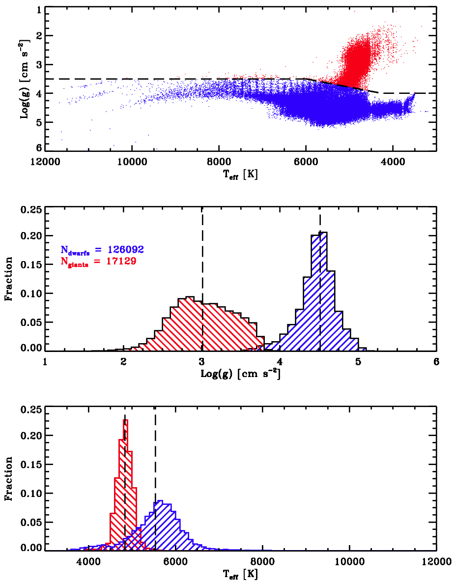
Figure 1.— Top: KIC-based Surface Gravity – Effective Temperature HR-diagram of the stars in the analysis sample. The dashed black line marks the delineation to separate dwarfs (blue) and giants (red). Center: Histograms of the surface gravity for the dwarfs (blue) and giants (red). The vertical dashed lines mark the median surface gravity values. Bottom: Histograms of the effective temperatures for the dwarfs (blue) and giants (red). The vertical dashed lines mark the median temperature values.

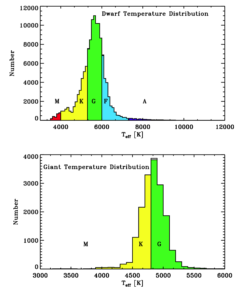
Figure 2.— Temperature distributions (binsize = 100 K) of the stars selected as dwarfs (top) and giants (bottom). The color-coding illustrates the separation of the dwarfs and giants into temperature groups (i.e., spectral types).

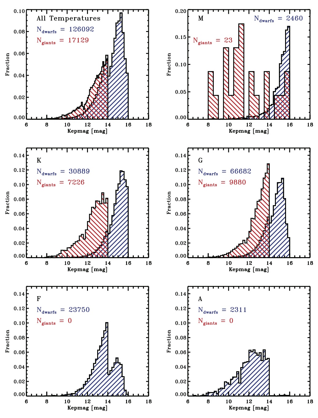
Figure 3.— Kepler magnitude distributions of the stars in the sample. Dwarfs and giants are represented by the blue and red hashed histograms, respectively. The panels represent the different temperature groups as labeled in the figures.

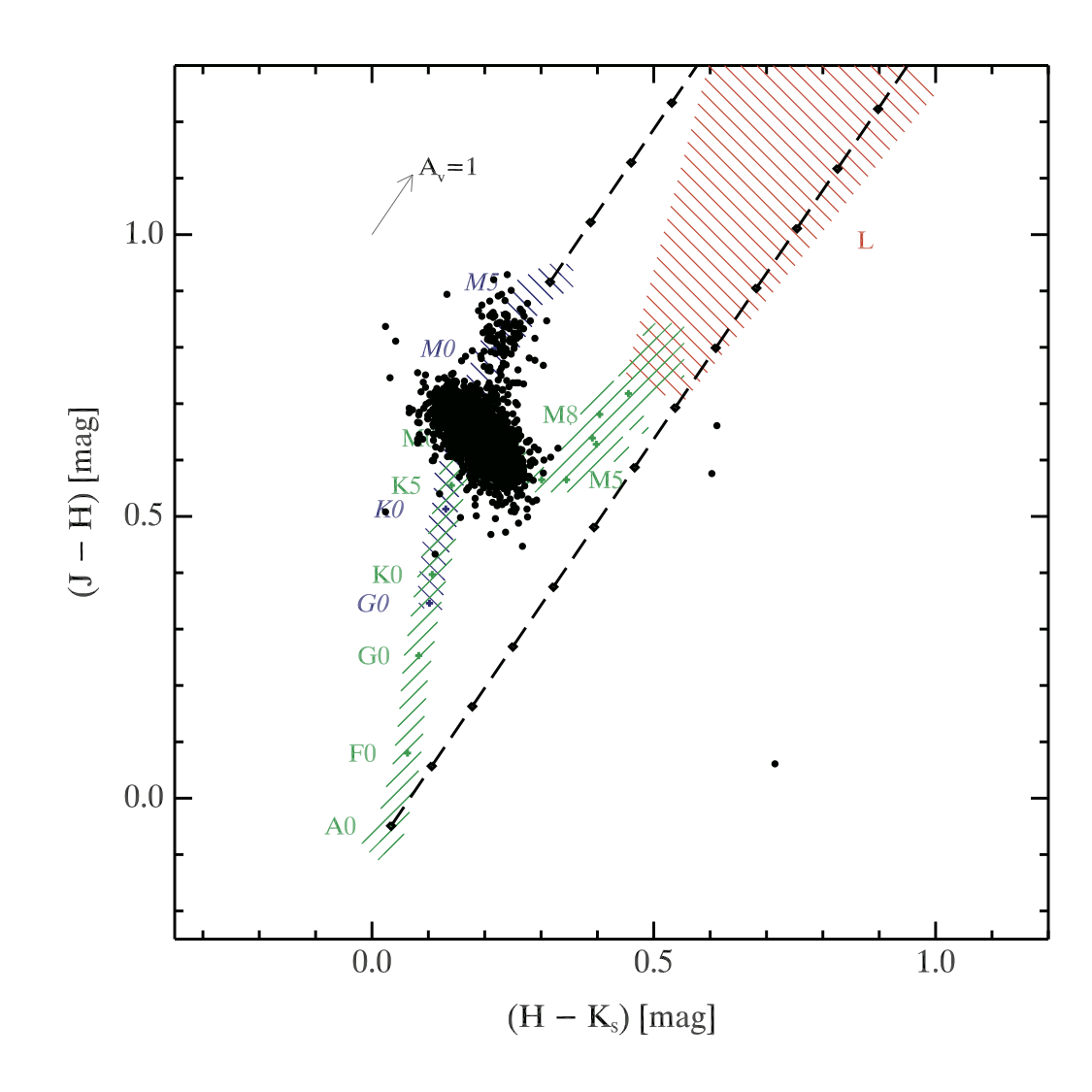
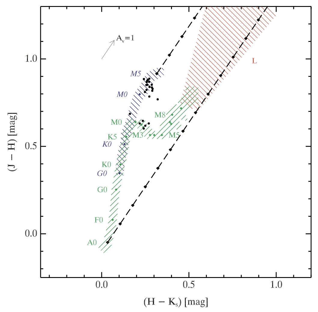
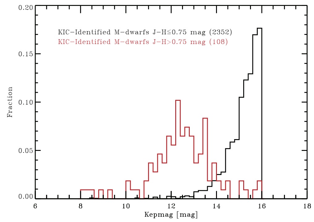
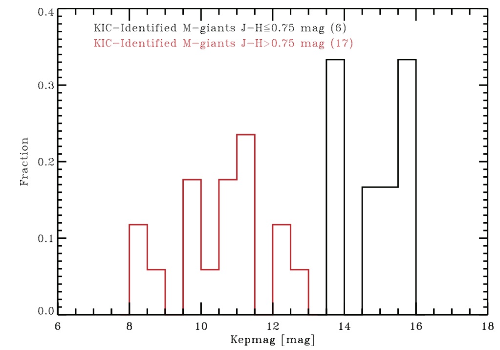
Figure 4.— Top: 2MASS color-color diagram for the stars identified as M-dwarfs (left) and M-giants (right) based upon the KIC surface gravities and effective temperatures. The green-hashed area marks the main sequence; the blue-hashed area marks the giant branch, and the red-hashed area marks the L-dwarf locus. The diagonal lines mark the reddening zone for typical galactic interstellar extinction (R=3.1). Bottom: Magnitude distributions for stars identified as dwarfs (left) and as giants (right) by their surface gravity. The black histograms are for stars with dwarf-like J-H colors; the red histograms are for stars with giant-like J-H colors. These plots show that the M-stars brighter $\sim$Kepmag$<13.5$ mag are predominately giants, regardless of their KIC classification.

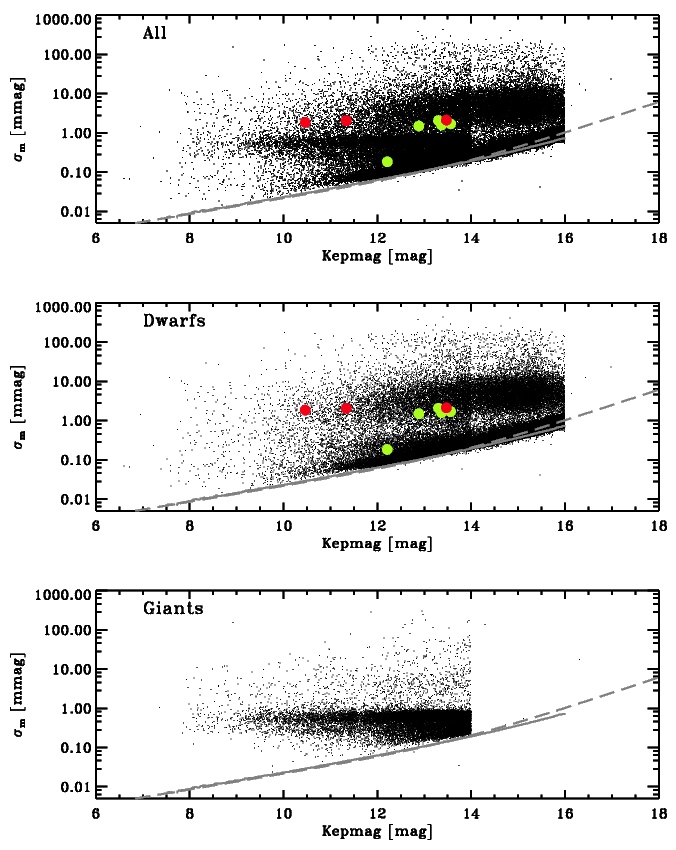
Figure 5.— Photometric dispersion (30 minute sampling; 33 day timescale) of each star is plotted as a function of magnitude for all stars (top), for just the dwarfs (center), and for just the giants (bottom). In the top and center plots, the locations of the 7 known planets in the sample are shown (red: BOKS-1, Hat-P7, and TrES-2; green: Kepler-4,5,6,7,8). The grey line represents the median uncertainty as reported in the Kepler data product. The dashed grey curve is the uncertainty upper limit curve from Jenkins et al. (2010).

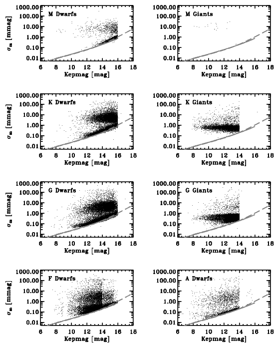
Figure 6.— Photometric dispersion (30 minute sampling; 33 day timescale) of each star is plotted as a function of magnitude separated out by temperature and surface gravity as labeled in each panel The solid grey line represents the median uncertainty value as reported in the Kepler data product. The dashed grey curve is the uncertainty upper limit curve from Jenkins et al. (2010).

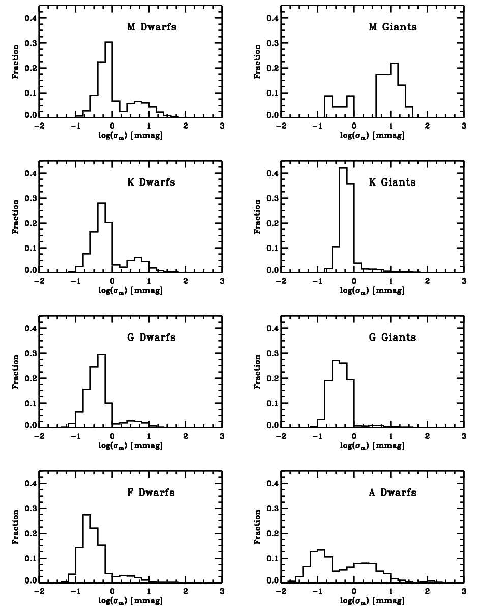
Figure 7.— Distributions of the (logarithmic) photometric dispersion (30 minute sampling; 33 day timescale) separated out by effective temperature and luminosity class as labeled in each panel.

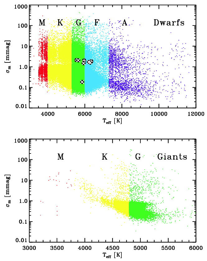
Figure 8.— Photometric dispersion (30 minute sampling; 33 day timescale) of each star is plotted as a function of effective temperature separated out by temperature (colors and labels) and surface gravity (top and bottom panels). The black points in the top panel mark the locations of the seven known planets in the sample ($+$: BOKS-1, HAT-P7, and TrES-2; $\times$: Kepler-4,5,6,7,8).

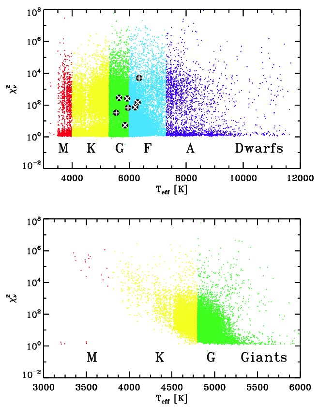
Figure 9.— Photometric reduced chi-square (30 minute sampling; 33 day timescale) of each star is plotted as a function of effective temperature separated out by temperature (colors and labels) and surface gravity (top and bottom panels). The black points in the top panel mark the locations of the seven known planets in the sample ($+$: BOKS-1, HAT-P7, and TrES-2; $\times$: Kepler-4,5,6,7,8).

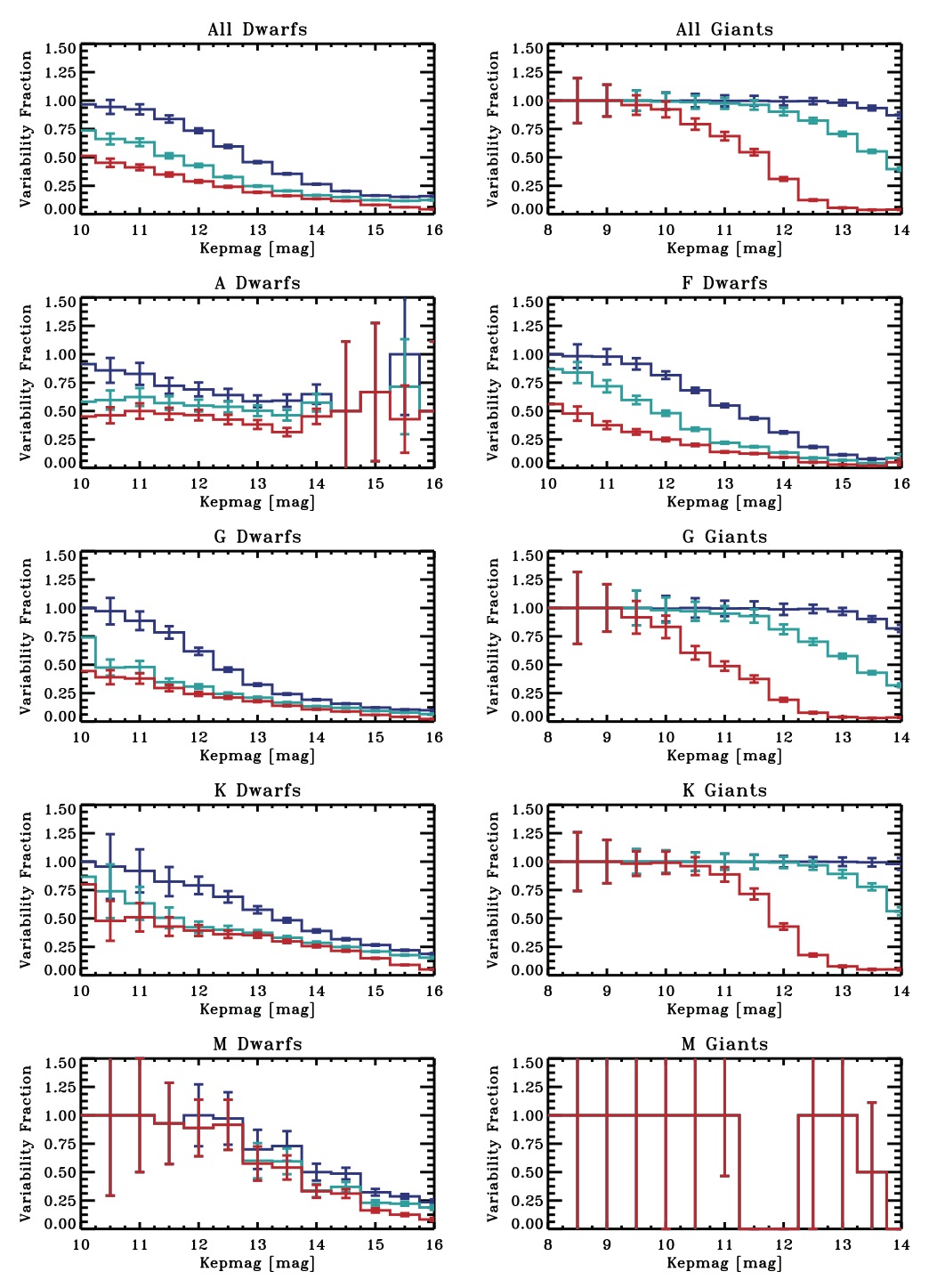
Figure 10.— Variability fractions of stars as a function of the brightness (Kepler magnitude). The contaminating giants in the M-dwarf sample and the contaminating dwarfs in the M-giant sample have been removed from the statistics. The blue curves represent the fractions of stars with $\chi^{2}_{\nu}>2$; the green curves represent the fractions of stars with $\chi^{2}_{\nu}>10$; the red curves represent the fractions of stars with $\chi^{2}_{\nu}>100$.

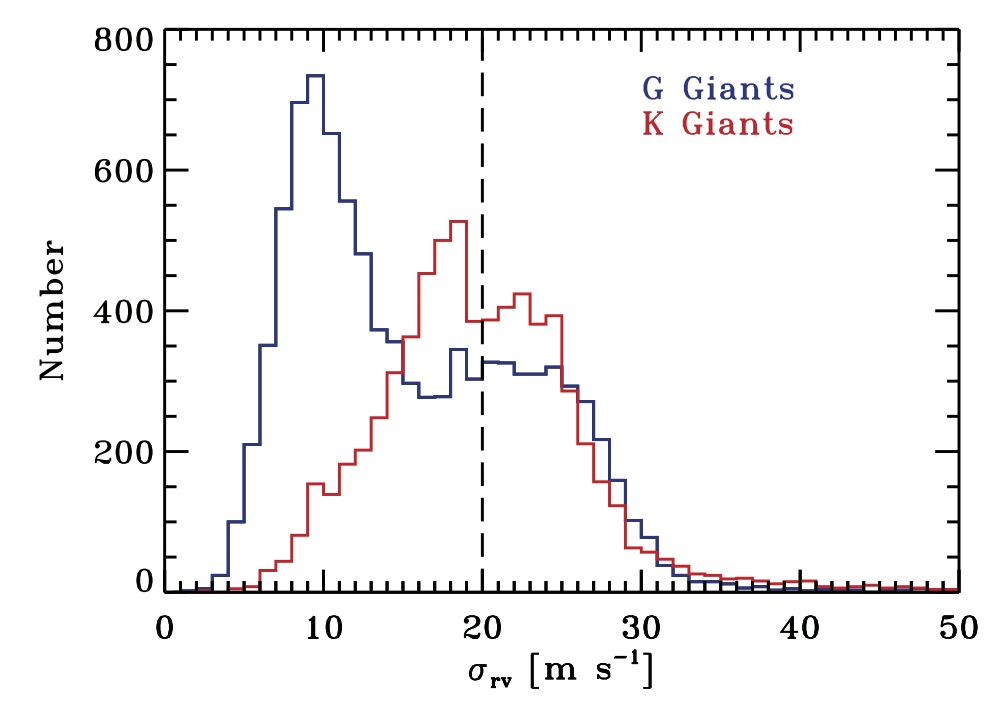
Figure 11.— Distribution of radial velocity oscillations of G (blue) and K (red) giants predicted from the photometric dispersion and effective temperature (Kjeldsen & Bedding, 1995). The dashed line marks the median radial velocity oscillation for the K-giant sample of Frink et al. (2001).

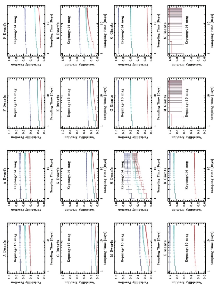
Figure 12.— Variability fraction distributions as a function of sampling. Each panel represents a different group of stars. There are two panels for each group; one panel for all the stars in the sample, and one panel where the stars were restricted to a Kepler magnitude of 14 or brighter. The contaminating giants in the M-dwarf sample and the contaminating dwarfs in the M-giant sample have been removed from the statistics. The blue curves represent the fractions of stars with $\chi^{2}_{\nu}>2$; the green curves represent the fractions of stars with $\chi^{2}_{\nu}>10$; the red curves represent the fractions of stars with $\chi^{2}_{\nu}>100$.

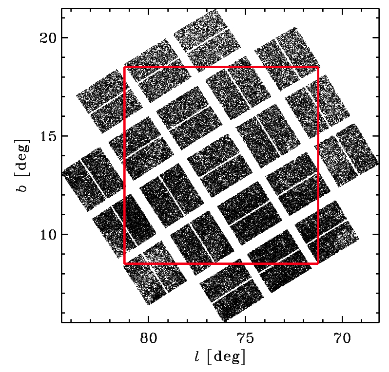
Figure 13.— Galactic coordinates plot of the positions of all the stars in the sample. The red-box delineates the $10^{\circ}\times 10^{\circ}$ region used to explore the variability as a function of galactic latitude.

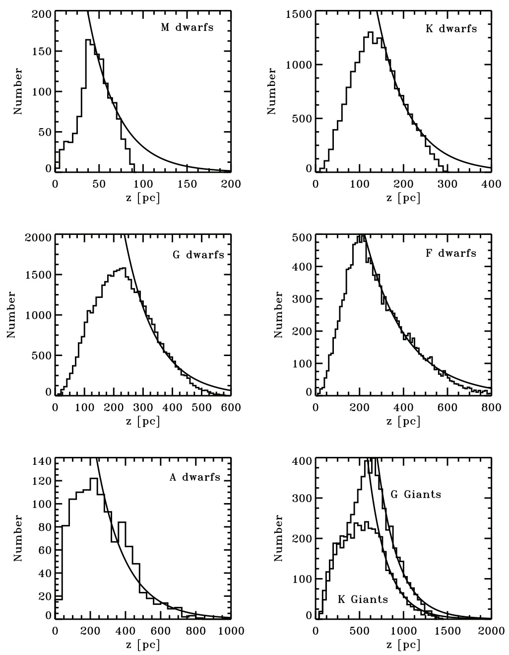
Figure 14.— $z$-height distributions for the dwarfs and G and K giants. The black smooth curves represent the best fit exponential curves to the distributions. The M-giants have been excluded from the plot because of the low number (23) in the sample.

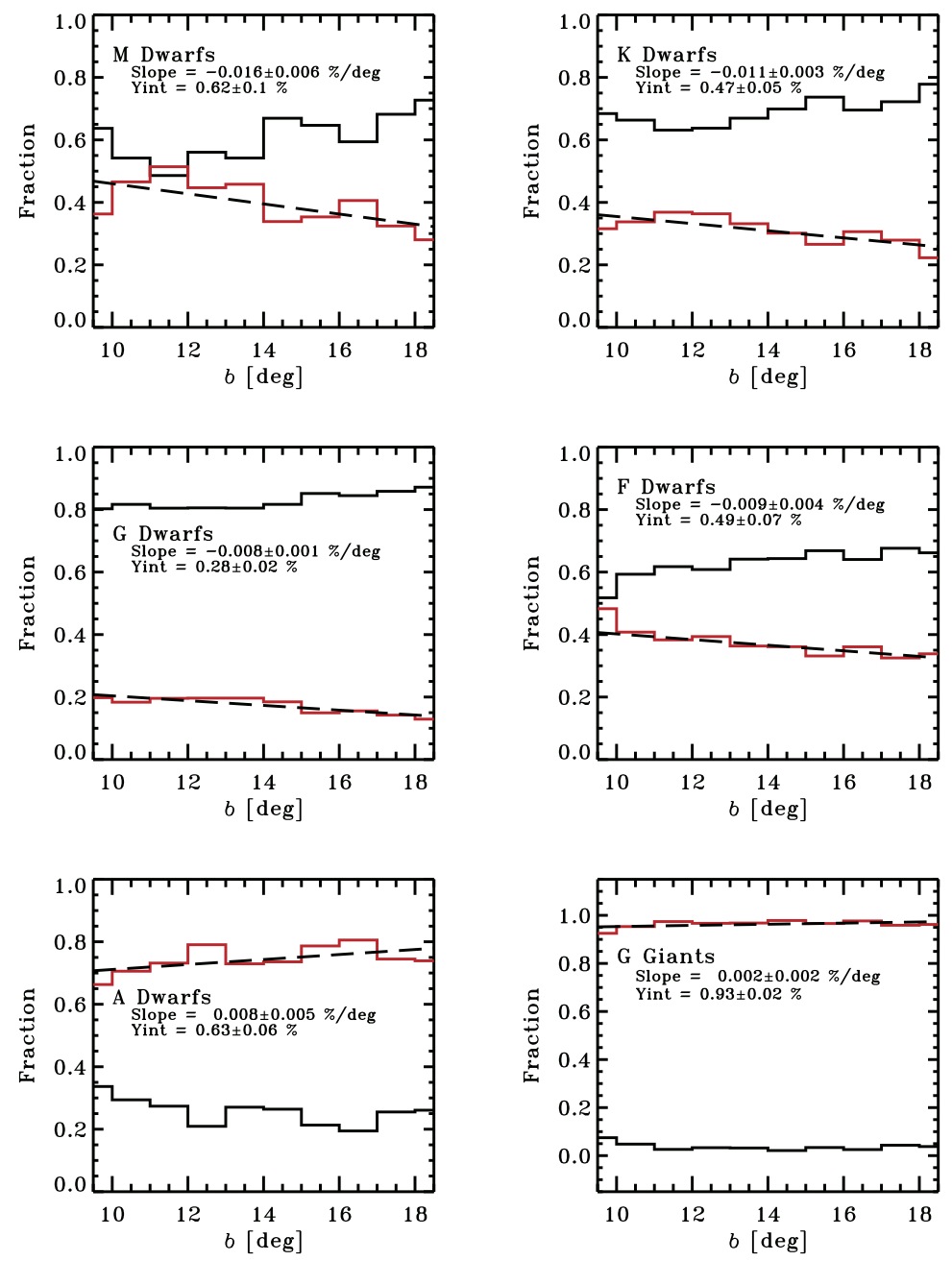
Figure 15.— Galactic latitude distributions (binsize=1^∘) for the dwarfs and G giants. The black curves represent the fraction of stars within that galactic latitude bin that are deemed “stable” ($\chi^{2}_{\nu}<2$), and the red curves represent the fraction of those stars that are deemed “variable” ($\chi^{2}_{\nu}>2$). The black dashed line is a best fit to the variability fraction as a function of galactic latitude with the parameters of the line fit given in each panel.

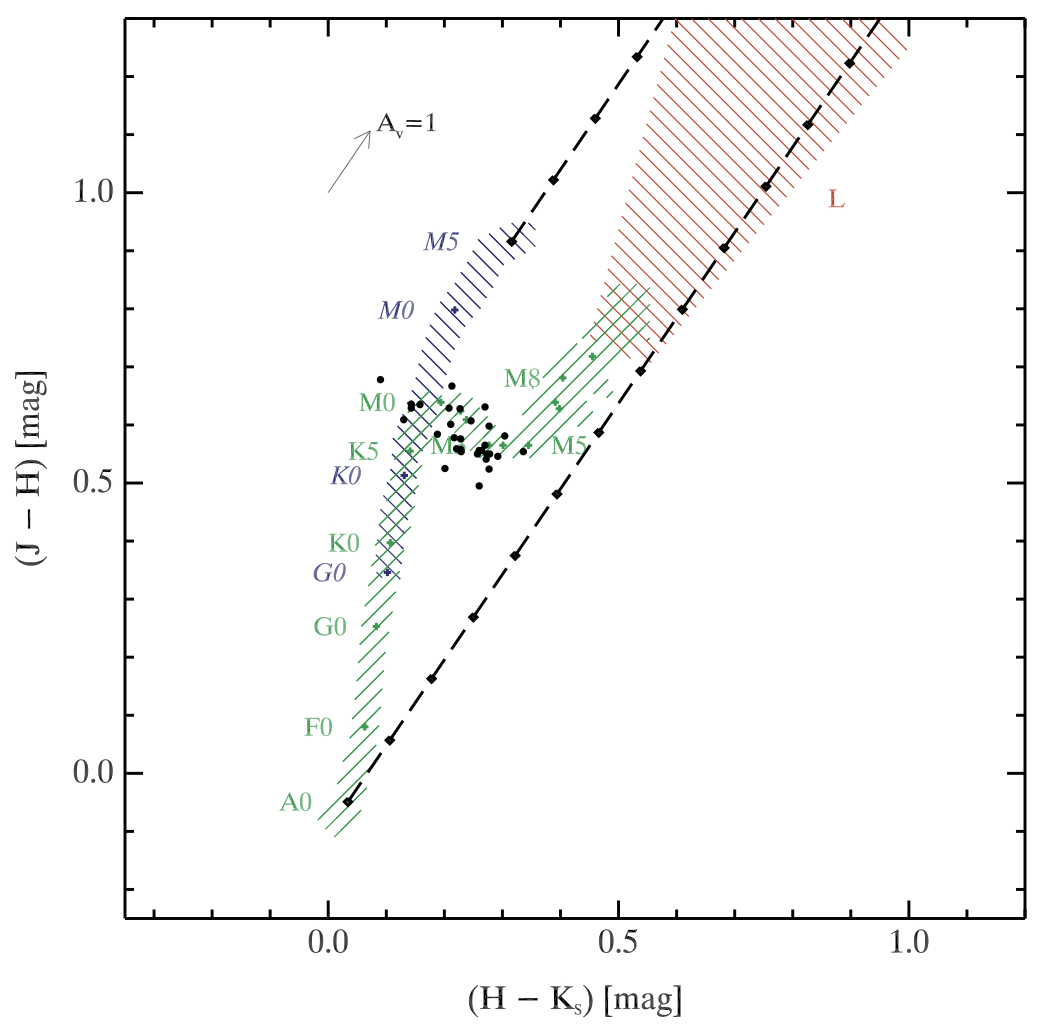
Figure 16.— 2MASS color-color diagram for the 29 stars identified as M-dwarfs from outside catalogs.

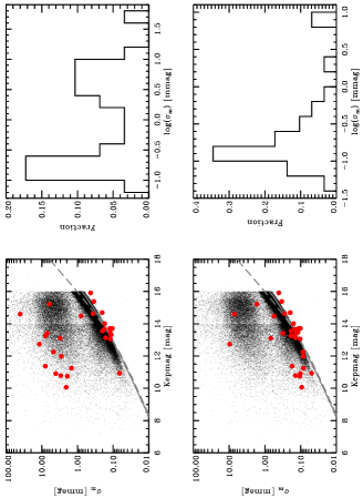
Figure 17.— Left panels show the photometric dispersion plotted as a function of magnitude for the KIC-identified M-dwarfs with a color restriction of J-H$<0.75$ mag (black dots) and for the outside identified M-dwarfs (red). The solid grey line represents the median uncertainty as reported in the Kepler data product. The dashed grey curve is the uncertainty upper limit curve from Jenkins et al. (2010). Right panels show the distributions of the (logarithmic) photometric dispersion (binsize = 0.2 dex) for the known M-dwarfs (red points in left figures). The top panels reflect the dispersion of the known M-dwarfs determined for the entire light curve (30 days); the bottom panels reflect the dispersion calculated from the point-to-point differences on 12-hour timescales (only for the known (red points) M-dwarfs). The KIC-identified M-dwarfs (black dots) are shown at the 30-minute cadence dispersion in both plots for reference.

References

- Auvergne et al. (2009) Auvergne, M. 2009, A&A, 506, 411
- Bakos et al. (2002) Bakos, G. Á., Sahu, K. C., & Németh, P. 2002, ApJS, 141, 187
- Basri et al. (2010a) Basri, G. et al. 2010a, ApJ, 713, L155
- Basri et al. (2010b) Basri, G. et al. 2010b, AJ, in press
- Batalha et al. (2010) Batalha, N. 2010, ApJ, 713, L109
- Bean et al. (2010) Bean, J. L., et al. 2010, ApJ, 713, 41
- Borucki et al. (2010) Borucki, W. J., et al. 2010, Science, 327, 977
- Castelli & Kurucz (2004) Castelli, F., & Kurucz, R. L. 2004, arXiv:astro-ph/0405087
- Charbonneau et al. (2009) Charbonneau, D., et al. 2009, Nature, 462, 891
- Ciardi et al. (1996) Ciardi, D. R. et al. 1996, AJ, 112, 700
- Drilling & Landolt (2000) Drilling, J. S. & Landolt, A. U. 2000, in Allen’s Astrophysical Quantities, 4th Edition, editor, Arthur N. Cox, 381
- Everett et al. (2002) Everett, M. E., Howell, S. B., van Belle, G. T., & Ciardi, D. R. 2002, PASP114, 656
- Eyer & Grenon (1997) Eyer, L., & Grenon, M. 1997, in Proc. ESA Symp. Hipparcos: Venice ’97, ed. B. Battrick (ESA SP-402; Noordwijk: ESA), 467
- Eyer & Mowlavi (2008) Eyer, L., & Mowlavi, N. 2008, Journal of Physics Conference Series, 118, 012010
- Feldmeier et al. (2010) Feldmeier, J. et al. AJ, in press
- Frink et al. (2001) Frink, S. et al. 2001, PASP, 113, 173
- Gilliland et al. (2008) Gilliland, R. L. 2008, AJ, 136, 566
- Haisch et al. (1999) Haisch, B. M. 1999, in The Many Faces of the Sun, ed. K. T. Strong, J.L. R. Saba, B. M. Haisch, & J. T. Schmelz (New York:Springer), 481
- Hartman et al. (2004) Hartman, J. D. et al. 2004, AJ, 128, 1761
- Henry et al. (2000) Henry, G. W. et al. 2000, ApJ, 130, 201
- Howell (2008) Howell, S. B. 2008, Astronomische Nachrichten, 329, 259
- Howell et al. (2010) Howell, S. B., et al. 2010, ApJ, 725, 1633
- Huber, Everett, & Howell (2006) Huber, M. E., Everett, M. E. & Howell, S. B. 2006, AJ, 132, 633
- Irwin et al. (2009) Irwin, J., Charbonneau, D., Nutzman, P., & Falco, E. 2009, IAU Symposium, 253, 37
- Jenkins et al. (2010) Jenkins, J. M., et al. 2010, ApJ, 713, L120
- Johnson (1966) Johnson, H. L. 1966,ARA&A,4, 193
- Johnson et al. (2010) Johnson, J. A. et al. 2010, ApJ, arXiv:1008.4141
- Jurić et al. (2008) Jurić, M., et al. 2008, ApJ, 673, 864
- Kabeth et al. (2009) Kabath, P. et al. 2009, A&A, 506, 569
- Kane et al. (2005) Kane, S. R. et al. 2005, MNRAS, 362, 117
- Kjeldsen & Bedding (1995) Kjeldsen, H. & Bedding, T. R., A&A, 293, 87
- Koch et al. (2010) Koch, D. G. et al. 2010, ApJ, 713, 79
- Latham et al. (2005) Latham, D. W. et al. 2005, BAAS, 37 1340
- Lépine (2005) Lépine, S. 2005, AJ, 130, 1680
- Majewski et al. (2000) Majewski, S. R., Ostheimer, J. C., Kunkel, W. E., & Patterson, R. J. 2000, AJ, 120, 2550
- Matthews et al. (1999) Matthews, J., et al. 1999, JRASC, 93, 183
- McCullough et al. (2005) McCoullough, P. R. et al. 2004, PASP, 117, 783
- O’Donovan et al. (2006) O’Donovan, F. T., et al. 2006, ApJ, 651, L61
- Pál et al. (2008) Pál, A., et al. 2008, ApJ, 680, 1450
- Pickering (1881) Pickering, E. C. 1881, Proc. Amer. Acad Arts & Sci., 16, 257
- Pojmanski (2002) Pojmanski, G. 2002, Acta Astronomica, 52, 397.
- Stauffer et al. (2010) Stauffer, J., et al. 2010a, PASP, 122, 885
- van Cleve (2010) van Cleve, J. 2010, “Kepler Data Release 6 Notes”
- Walkowicz et al. (2010) Walkowicz, L. M. et al. 2010, ApJ, submitted
- Wozniak & Szymanski (1998) Wozniak, P., & Szymanski, M. 1998, Acta Astronomica, 48, 269
- West et al. (2008) West, A. A. et al. 2008, AJ, 135, 785