Non-decoupling effects in supersymmetric Higgs sectors

Abstract

A wide class of Higgs sectors is investigated in supersymmetric standard models. When the lightest Higgs boson ($h$) looks the standard model one, the mass ($m_{h}$) and the triple Higgs boson coupling (the $hhh$ coupling) are evaluated at the one-loop level in each model. While $m_{h}$ is at most 120-130 GeV in the minimal supersymmetric standard model (MSSM), that in models with an additional neutral singlet or triplet fields can be much larger. The $hhh$ coupling can also be sensitive to the models: while in the MSSM the deviation from the standard model prediction is not significant, that can be 30-60 % in some models such as the MSSM with the additional singlet or with extra doublets and charged singlets. These models are motivated by specific physics problems like the $\mu$-problem, the neutrino mass, the scalar dark matter and so on. Therefore, when $h$ is found at the CERN Large Hadron Collider, we can classify supersymmetric models by measuring $m_{h}$ and the $hhh$ coupling accurately at future collider experiments.

I Introduction

Physics of electroweak symmetry breaking (EWSB) is the last unknown part in the standard model (SM). Experimental identification of the Higgs sector has been one of the most important issues in high energy physics. Yet no Higgs boson has been found at the CERN LEP and the Fermilab Tevatron, the data are used to constrain the Higgs boson parameters LEP ; Tevatron . The Higgs boson search has also started at the CERN Large Hadron Collider (LHC). When a scalar boson is found in near future, its property will be measured as accurately as possible to see whether the scalar is really the Higgs boson. In particular, to understand the essence of EWSB, we must know the self-coupling in addition to the Higgs boson mass. The triple Higgs boson coupling may be explored at the LHC and its upgraded versionhhh_lhc , the International Linear Collider (ILC)hhh_lc and its $\gamma\gamma$ optiongammagamma or the Compact Linear Collider (CLIC).

Experimental survey for the Higgs sector is important not only to confirm our picture for EWSB, but also to explore new physics beyond the SM (BSM). In the SM, appearance of the quadratic ultraviolet divergence in the one-loop calculation of the Higgs boson mass is a serious problem, which is called the hierarchy problem. This has to be eliminated in a model of BSM. On the other hand, we already know several phenomena of BSM such as dark matter, tiny neutrino masses, and baryon asymmetry of the universe.

Supersymmetry (SUSY) is an attractive idea as a new physics scenario at the TeV scale. First of all, the hierarchy problem can be solved: i.e., the quadratic divergence due to a particle in the loop is cancelled by that due to the super partner particles. Second, a supersymmetric standard model (SSM) can naturally contain the candidate for dark matter; i.e., the lightest SUSY particle, whose stability may be guaranteed by the R-parity. One of the important predictions in the minimal SSM (MSSM), where the Higgs sector is composed of two Higgs doublets, is to the mass ($m_{h}$) of the lightest CP-even Higgs boson ($h$), which is predicted to be less than the $Z$ boson mass ($m_{Z}$) at the tree level, but can be maximally 30-40 GeV above $m_{Z}$ by radiative effects of the top quark and its super partners (stops) mass_mssm . This prediction meets the present LEP bound on $m_{h}$ LEP . If such a light $h$ will not be found, the MSSM must be ruled out. Is SUSY itself ruled out then? The answer is “No”. In fact, there can be several variations for the Higgs sector in SSMs. A simple extension may be addition of a neutral gauge singlet field to the MSSM, which is known as the Next-to MSSM (NMSSM) nmssm ; nmssm_mh ; ellwanger . Solving the $\mu$ problem mu-problem may be a motivation to the NMSSM. It is known that $m_{h}$ in the NMSSM can be higher than that in the MSSM because of the additional contribution to $m_{h}$ from the tri-linear term of the Higgs doublets and the singlet in the superpotential. In addition to the MSSM and the NMSSM, a model with additional scalar boson with higher representation can also push up $m_{h}$tripletmh . Furthermore, models with extended gauge sector can also have higher $m_{h}$ than the MSSM predictionextragauge , depending on the model parameters. Therefore, $m_{h}$ can be an important tool to discriminate SSMs.

In this Letter, we investigate Higgs sectors in a wide class of SSM, when only the lightest Higgs boson $h$ appears at the electroweak (EW) scale and the other additional particles such as extra Higgs bosons and SUSY partner particles are rather heavier (but not too heavy). The coupling constants of $h$ to the SM particles are then similar to those in the SM at the tree level. In each model, $m_{h}$ as well as the deviation in the triple Higgs boson coupling (the $hhh$ coupling) are evaluated at the one-loop level. Their possible allowed values as well as their correlation are studied under the theoretical condition and the current experimental data. We here consider not only the MSSM and the NMSSM, but also further possible extensions of the MSSM. In order to widely examine various possibilities, we here do not necessarily require the paradigm of the grand unification. Instead, we may even retain the possibility of appearance of strong dynamics at the TeV scale as discussed in Ref. fat_higgs .

II Extended SUSY Models

One way of the extension of the MSSM may be adding new chiral superfields such as isospin singlets (neutral $S$, singly charged $\Omega_{\pm}$ or doubly charged $K_{\pm}$), doublets ($H_{u}^{\prime}$ and $H_{d}^{\prime}$), or triplets ($\xi$ with the hypercharge $Y=0$ or $\chi_{\pm}$ with $Y=\pm 1$), whose properties are defined in Table 1. As we are interested in the variation in the Higgs sector, these new fields are supposed to be colour singlet. Although there can be further possibilities such as introduction of new vector superfields which contain gauge fields for extra gauge symmetries, models with extra dimensions, those with the R-parity violation, etc, we here do not discuss them. Eventually, in addition to the MSSM, we consider nine models in Table 2. In the analysis of this letter, triple coupling terms with doublet Higgs superfields and additional chiral superfields play an important role. In Table 2, such relevant terms are also listed. For anomaly cancellation, charged superfields are introduced in pair in each model.

These extensions can be motivated by solving various physics problems. For example, models with additional charged singlet fields can be used for radiative neutrino mass generation radiative_seesaw . Those with additional doublet fields may be required for dark doublet models dark_higgs , and the model with triplets may be motivated for the SUSY left-right modelLRmodels or those with so-called the type-II seesaw mechanism type-II_seesaw . Although models in Table 2 can be imposed additional exact or softly-broken discrete symmetries for various reasons, we here do not specify them as they do not affect our discussions.

	$S$	$\Omega_{+}$	$\Omega_{-}$	$K_{+}$	$K_{-}$	$H_{u}^{\prime}$	$H_{d}^{\prime}$	$\xi$	$\chi_{+}$	$\chi_{-}$
SU(2)I	1	1	1	1	1	2	2	3	3	3
U(1)Y	0	1	$-1$	2	$-2$	$1/2$	$-1/2$	0	1	$-1$

Table 1: Properties of additional chiral superfields.

	$S$	$\Omega_{+}$	$\Omega_{-}$	$K_{+}$	$K_{-}$	$H_{u}^{\prime}$	$H_{d}^{\prime}$	$\xi$	$\chi_{+}$	$\chi_{-}$	Relevant terms in the superpotential
Model-1	$\bullet$										$W\supset\lambda_{HHS}H_{u}\cdot H_{d}S$
Model-2								$\bullet$			$W\supset\lambda_{HH\xi}H_{u}\cdot\xi H_{d}$
Model-3		$\bullet$	$\bullet$								—
Model-4		$\bullet$	$\bullet$	$\bullet$	$\bullet$						—
Model-5									$\bullet$	$\bullet$	$W\supset\frac{\lambda_{HH\chi_{-}}}{2}H_{u}\cdot\chi_{-}H_{u}+\frac{\lambda_{HH\chi_{+}}}{2}H_{d}\cdot\chi_{+}H_{d}$
Model-6						$\bullet$	$\bullet$				—
Model-7	$\bullet$					$\bullet$	$\bullet$				$W\supset\lambda_{H_{u}H_{d}S}H_{u}\cdot H_{d}S+\lambda_{H_{u}^{\prime}H_{d}S}H_{u}^{\prime}\cdot H_{d}S$
											$\phantom{W\supset}+\lambda_{H_{u}H_{d}^{\prime}S}H_{u}\cdot H_{d}^{\prime}S+\lambda_{H_{u}^{\prime}H_{d}^{\prime}S}H_{u}^{\prime}\cdot H_{d}^{\prime}S$
Model-8						$\bullet$	$\bullet$	$\bullet$			$W\supset\lambda_{H_{u}H_{d}\xi}H_{u}\cdot\xi H_{d}+\lambda_{H_{u}^{\prime}H_{d}\xi}H_{u}^{\prime}\cdot\xi H_{d}$
											$\phantom{W\supset}+\lambda_{H_{u}H_{d}^{\prime}\xi}H_{u}\cdot\xi H_{d}^{\prime}+\lambda_{H_{u}^{\prime}H_{d}^{\prime}\xi}H_{u}^{\prime}\cdot\xi H_{d}^{\prime}$
Model-9		$\bullet$	$\bullet$			$\bullet$	$\bullet$				$W\supset\lambda_{HH\Omega_{-}}H_{u}\cdot H_{u}^{\prime}\Omega_{-}+\lambda_{HH\Omega_{+}}H_{d}\cdot H_{d}^{\prime}\Omega_{+}$

Table 2: Particle entries in each SSM. Additional terms in the superpotential which are relevant to the extra chiral superfields are also shown in each model.

III The method

The effective potential for the order parameter $\varphi$ can be written at the one-loop order asSU2U1potential

$$V_{\rm eff}(\varphi)=-\frac{\mu_{0}^{2}}{2}\varphi^{2}+\frac{\lambda_{0}}{4}\varphi^{4}+\sum_{f}\frac{(-1)^{2s_{f}}N_{C_{f}}N_{S_{f}}}{64\pi^{2}}m_{f}(\varphi)^{4}\left[\ln\frac{m_{f}(\varphi)^{2}}{Q^{2}}-\frac{3}{2}\right],$$ (1)

where $\mu_{0}^{2}$ and $\lambda_{0}$ are the bare squared mass and the coupling constant, $m_{f}(\varphi)$ is the field dependent mass of the field $f$ in the loop, and $N_{C_{f}}$ and $N_{S_{f}}$ are the degree of freedom of the colour and the spin with $s_{f}$ being the spin of the field $f$. In SSMs, the Higgs sector has a multi-Higgs structure. When the extra Higgs scalars are heavy enough, only the lightest Higgs boson $h$ stays at the EW scale, and behaves as the SM-like one. The effective potential in Eq. (1) can then be applied with a good approximation. The vacuum, the mass $m_{h}$ and the $hhh$ coupling constant $\lambda_{hhh}$ are determined at the one-loop order by the conditions;

$$\left.\frac{\partial V_{\rm eff}}{\partial\varphi}\right|_{\varphi=v}=0,\hskip 5.69054pt\left.\frac{\partial^{2}V_{\rm eff}}{\partial\varphi^{2}}\right|_{\varphi=v}=m_{h}^{2},\hskip 5.69054pt\left.\frac{\partial^{3}V_{\rm eff}}{\partial\varphi^{3}}\right|_{\varphi=v}=\lambda_{hhh},$$ (2)

where $v$ ($\simeq 246$ GeV) is the vacuum expectation value for the EWSB.

IV The Mass and the triple coupling of the lightest Higgs bosons

IV.1 The Mass of the lightest Higgs boson

In the MSSM, $m_{h}$ is evaluated by using Eq. (2) as

$$m_{h}^{2}=m_{Z}^{2}\cos^{2}2\beta+\delta m_{\rm loop}^{2},$$ (3)

where $\tan\beta\equiv\langle H_{u}^{0}\rangle/\langle H_{d}^{0}\rangle$. The first term of the R.H.S. comes from the D-term at the tree level. The quantum correction $\delta m_{\rm loop}^{2}$ has turned out to be important mass_mssm ; mssm_mh to satisfy the LEP data ($m_{h}>114$ GeV) LEP ;

$$\delta m_{\rm loop}^{2}\simeq\frac{3m_{t}^{4}}{4\pi^{2}v^{2}}\ln\frac{m_{\tilde{t}_{1}}^{2}m_{\tilde{t}_{2}}^{2}}{m_{t}^{4}}+\frac{3m_{t}^{2}X_{t}^{2}\sin^{2}\beta}{4\pi^{2}(m_{\tilde{t}_{2}}^{2}-m_{\tilde{t}_{1}}^{2})}\ln\frac{m_{\tilde{t}_{2}}^{2}}{m_{\tilde{t}_{1}}^{2}}+\mathcal{O}(X_{t}^{3}/m_{\tilde{t_{i}}}^{3}),$$ (4)

where $m_{t}$ is the top quark mass, $m_{\tilde{t}_{1,2}}$ are the masses of stops $\tilde{t}_{1}$ and $\tilde{t}_{2}$ ($m_{\tilde{t}_{1}}<m_{\tilde{t}_{2}}$), and $X_{t}$ is defined such that the coupling constant of $\tilde{t}_{L}$-$\tilde{t}_{R}$-$h$ is given by $X_{t}\sin\beta/\sqrt{2}$. Because the top Yukawa coupling is of order one, $\delta m_{\text{loop}}^{2}$ can push up the upper bound to 120-130GeV when stop masses are of order one TeV. Higher order calculations for $m_{h}$ have been studied in literaturehighloopmh .

	Squared mass ($m_{h}^{2}$) of the SM-like Higgs boson $h$	Ratio of the $hhh$ coupling: $\lambda_{hhh}^{\rm Model}/\lambda_{hhh}^{\rm SM}$
MSSM
Model-3	$\displaystyle\simeq m_{Z}^{2}\cos^{2}2\beta+\delta m_{\rm loop}^{2}$	$\displaystyle\simeq 1+{\cal O}\left(\frac{v^{2}}{m_{\rm SUSY}^{2}}\right)$
Model-4
Model-6
Model-1	$\displaystyle\simeq m_{Z}^{2}\cos^{2}2\beta$	$\displaystyle\simeq 1+\sum_{c=1}^{2}\ \frac{m_{S_{c}}^{4}}{12\pi^{2}v^{2}m_{h}^{2}}\left(1-\frac{M_{S_{c}}^{2}}{m_{S_{c}}^{2}}\right)^{3}$
	$\displaystyle+\sum_{c=1}^{2}\frac{m_{S_{c}}^{2}}{2}\left(1-\frac{M^{2}_{S_{c}}}{m_{S_{c}}^{2}}\right)\sin^{2}2\beta+\delta\overline{m}_{\text{loop}}^{2}(\text{Model-1})$
Model-5	$\displaystyle\simeq m_{Z}^{2}\cos^{2}2\beta$
	$\displaystyle+\sum_{i=\pm}\sum_{c=1}^{4}\frac{m_{T_{i}^{c}}^{2}}{4}\left(1-\frac{M_{T_{i}^{c}}^{2}}{m_{T_{i}^{c}}^{2}}\right)C_{i}+\delta\overline{m}_{\text{loop}}^{2}(\text{Model-5})$	$\displaystyle\simeq 1+\sum_{i=\pm}\sum_{c=1}^{4}\frac{m_{T_{i}^{c}}^{4}}{12\pi^{2}v^{2}m_{h}^{2}}\left(1-\frac{M_{T_{i}^{c}}^{2}}{m_{T_{i}^{c}}^{2}}\right)^{3}$
Model-9	$\displaystyle\simeq m_{Z}^{2}\cos^{2}2\beta+\delta m_{\rm loop}^{2}$	$\displaystyle\simeq 1+\sum_{i=\pm}\sum_{c=1}^{2}\frac{m_{\Omega_{i}}^{4}}{12\pi^{2}v^{2}m_{h}^{2}}\left(1-\frac{M_{\Omega_{i}}^{2}}{m_{\Omega_{i}}^{2}}\right)^{3}$

Table 3: Formulae for $m_{h}$ and $\lambda_{hhh}^{\rm Model}/\lambda_{hhh}^{\rm SM}$ in various SSMs at the one-loop orderksy_full . Masses of the component fields $S_{c}$, $T_{i}^{c}$, and $\Omega_{i}$ are given by $m_{S_{c}}$, $m_{T^{c}_{i}}$ and $m_{\Omega_{i}}$, while $M_{\phi_{i}^{c}}^{2}=m_{\phi_{i}^{c}}^{2}-\lambda_{HH\phi_{i}}^{2}v^{2}C_{i}/2$, where $\phi_{i}^{c}=S_{c}$, $T_{i}^{c}$, or $\Omega_{i}$ and $C_{-}=\sin^{2}\beta$ and $C_{+}=\cos^{2}\beta$ in both Model-5 and Model-9 and $C_{i}=1$ in the other models. In Model-2, Model-7 and Model-8, there are similar non-decoupling effects to Model-1.

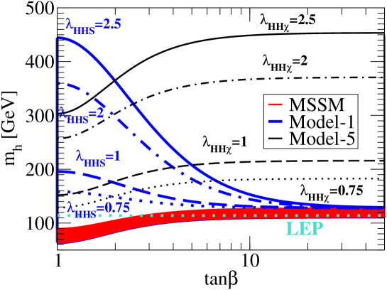
Figure 1: The upper bounds on $m_{h}$ as a function of $\tan\beta$ for fixed values of $\lambda_{HHS}$ and $\lambda_{HH\chi_{-}}=\lambda_{HH\chi_{+}}\equiv\lambda_{HH\chi}$ in Model-1 and Model-5, respectively. The red-filled region indicates the possible allowed region in the MSSM.

In general cases with additional chiral superfields, the F-term can also contribute to $m_{h}$ at the tree level. For example, in Model-1 (i.e., the NMSSM), the term of $\lambda_{HHS}H_{u}\cdot H_{d}S$ in the superpotential gives the coupling of $\lambda_{HHS}^{2}(H_{u}\cdot H_{d})^{2}$ in the Higgs potential, which yields

$$m_{h}^{2}\simeq m_{Z}^{2}\cos^{2}2\beta+(\lambda_{HHS}^{2}v^{2}/2)\sin^{2}2\beta+\delta\overline{m}_{\text{loop}}^{2}(\text{Model-1}),$$ (5)

where

$$\delta\overline{m}_{\text{loop}}^{2}(\text{Model-1})=\delta m_{\rm loop}^{2}+\frac{\lambda_{HHS}^{4}v^{2}}{32\pi^{2}}\ln\frac{m_{S_{1}}^{2}m_{S_{2}}^{2}}{m_{\tilde{S}}^{4}}\;,$$ (6)

where $m_{S_{1}}$, $m_{S_{2}}$, and $m_{\tilde{S}}$ are masses of a CP-even scalar component, a CP-odd scalar component and a fermion component of $S$, respectively. We here assume that the mixing between component fields are so small that each component field can be regarded as a mass eigenstate. We consider the case that the scalar and the fermion components of the additional fields are approximately degenerate and the logarithmic correction from them are negligible. Due to the $\lambda_{HHS}^{2}$ term, $m_{h}$ can be above 130 GeV. It is bounded from above by the renormalization group equation analysis assuming the condition of avoiding the Landau pole below a given value of $\Lambda$ triviality ; nmssm_mh . The upper bound of $m_{h}$ is evaluated to be about 140 GeV at $\tan\beta\simeq 2$ (about 450 GeV at $\tan\beta\simeq 1$) for $\Lambda\simeq 10^{16}$ GeV (4 TeV)ellwanger .

Similarly, the enhancement of $m_{h}$ due to the F-term contribution can also be realized in models with an additional field $\phi$ where the superpotential has the gauge singlet operator like $H_{u}H_{d}\phi$. In Table 2, Model-1, Model-2, Model-5, Model-7 and Model-8 satisfy this condition, where $m_{h}$ receives the F-term contribution and can be significantly larger than that in the MSSM. Approximate formulae for $m_{h}$ are given in Table 3.

In Fig. 1, the upper bounds on $m_{h}$ in Model-1 and Model-5 are shown as a function of $\tan\beta$, and the possible allowed region in the MSSM is also indicated by the red-filled region. The coupling constants $\lambda_{HH\phi}$ ($\phi=S$ and $\chi_{\pm}$) are taken as $0<\lambda_{HH\phi}<2.5$, whose upper limit corresponds to $\Lambda\gtrsim 4$ TeV in Model-1 for the case with the typical scale of the soft SUSY breaking to be $500$ GeV. The detail is shown elsewhere ksy_full . In Model-1 with a fixed value of $\lambda_{HHS}$, $m_{h}$ can be maximal for $\tan\beta=1$, while in Model-5 it becomes maximal for large values of $\tan\beta$ for a fixed value of $\lambda_{HH\chi}$. The maximal value in Model-1 becomes asymptotically the same as that in the MSSM in the large $\tan\beta$ limit up to the one-loop logarithmic contributions.

IV.2 The $hhh$ coupling

We turn to the discussion on the quantum effect on the $hhh$ coupling in the SSMs in the case where $h$ is regarded as the SM like Higgs boson. To this end, we start from the case in the non-SUSY extended Higgs sector. It is known that in the non-SUSY two Higgs doublet model (THDM), the $hhh$ coupling can receive large non-decoupling effects from the loop contribution of extra Higgs bosons, when their masses are generated mainly by EWSB KKOSY ; nondec . When $h$ is the SM like Higgs boson, physical masses of the extra scalar bosons are expressed by

$$m_{\Phi_{i}}^{2}=M^{2}+\frac{\lambda_{i}v^{2}}{2}\;,$$ (7)

where $\Phi_{i}$ represents $H^{0}$, $H^{\pm}$ or $A^{0}$, and $M$ is the invariant mass scale which is irrelevant to the EWSB, and $\lambda_{i}$ is a coupling for $\Phi_{i}^{\dagger}\Phi_{i}hh$. The physical meaning of $M$ is discussed in, for example, Ref. KKOSY ; nondec . The one-loop contribution to the renormalized $hhh$ coupling is calculated asKKOSY ; nondec

$$\frac{\lambda_{hhh}^{\text{THDM}}}{\lambda_{hhh}^{\text{SM}}}\simeq 1+\frac{1}{12\pi^{2}m_{h}^{2}v^{2}}\left\{m_{H^{0}}^{4}\left(1-\frac{M^{2}}{m_{H^{0}}^{2}}\right)^{3}+m_{A^{0}}^{4}\left(1-\frac{M^{2}}{m_{A^{0}}^{2}}\right)^{3}+2m_{H^{\pm}}^{4}\left(1-\frac{M^{2}}{m_{H^{\pm}}^{2}}\right)^{3}\right\}\;.$$ (8)

One finds that for $M^{2}\gg\lambda_{i}v^{2}$ it becomes

$$\frac{\lambda_{hhh}^{\text{THDM}}}{\lambda_{hhh}^{\text{SM}}}\simeq 1+\frac{v^{2}}{96\pi^{2}m_{h}^{2}}\left(\lambda_{H^{0}}^{3}+\lambda_{A^{0}}^{3}+2\lambda_{H^{\pm}}^{3}\right)\left(\frac{v^{2}}{M^{2}}\right)\;,$$ (9)

which vanishes in the large $M$ limit according to the Appelquist-Carazzone decoupling theoremAppelquist . On the contrary, when the physical scalar masses are mainly determined by the $\lambda_{i}v^{2}$ term, the loop contribution to the $hhh$ coupling does not decouple, and the quartic powerlike contributions of $m_{\Phi_{i}}$ remain;

$$\frac{\lambda_{hhh}^{\text{THDM}}}{\lambda_{hhh}^{\text{SM}}}\simeq 1+\frac{1}{12\pi^{2}m_{h}^{2}v^{2}}\left(m_{H^{0}}^{4}+m_{A^{0}}^{4}+2m_{H^{\pm}}^{4}\right)\;.$$ (10)

Consequently, a significant quantum effect can be realized for the $hhh$ coupling when $m_{\Phi_{i}}^{2}>m_{h}^{2}$. The size of the correction from the SM value can be of 100% for $m_{h}=120$GeV, $M\simeq 0$, and $m_{H^{0}}\simeq m_{A^{0}}\simeq m_{H^{\pm}}\simeq 400$GeV under the constraint from perturbative unitarityKKT . Such a large non-decoupling effect on the $hhh$ coupling is known to be related to the strongly first order EW phase transition ewbg-thdm2 which is required for the EW baryogenesisewbg-thdm .

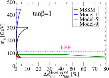
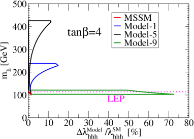
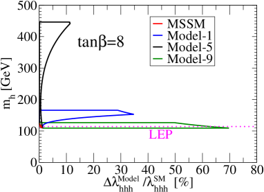
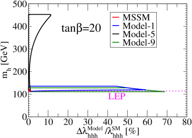
Figure 2: Possible allowed regions in the $m_{h}$-$(\Delta\lambda_{hhh}/\lambda_{hhh})$ plane in the MSSM, Model-1, Model-5 and Model-9 for each $\tan\beta$ value. We scan the parameter space as $0<\lambda_{HH\phi}<2.5$, $0.5\,\text{TeV}<m_{\tilde{t}_{1,2}}<1.5\,\text{TeV}$, and $0.5\,\text{TeV}<m_{\phi_{i}^{c}}$ for each model.

Let us discuss the $hhh$ coupling in the SSMs listed in Table 2. In the MSSM, it is evaluated at the one-loop level as

$$\lambda^{\rm{MSSM}}_{hhh}\simeq\frac{3m_{h}^{2}}{v}\left[1-\frac{m_{t}^{4}}{\pi^{2}v^{2}m_{h}^{2}}\left\{1-\frac{m_{t}^{2}(m_{\tilde{t}_{1}}^{2}+m_{\tilde{t}_{2}}^{2})}{2m_{\tilde{t}_{1}}^{2}m_{\tilde{t}_{2}}^{2}}+\frac{3X_{t}^{2}v^{2}\sin^{2}\beta}{4m_{\tilde{t}_{1}}^{2}m_{\tilde{t}_{2}}^{2}}\right\}\right],$$ (11)

up to the stop mixing ewbg-thdm2 . This result coincides with that in the SM in the decoupling limit $m_{\tilde{t}_{1,2}}\rightarrow\infty$ KKOSY ; nondec . On the contrary, in a class of the SSMs; Model-1, Model-5 and Model-9, the non-decoupling effect can appear in the $hhh$ coupling, similarly to the case of the THDM. Approximate formulae of the $\lambda_{hhh}^{\rm Model}/\lambda_{hhh}^{\rm SM}$ are given in Table 3. In the following, we explain the results in each model in order.

In Model-1 a scalar boson $S_{1}$ and a pseudo-scalar boson $S_{2}$ from extra isospin singlet field $S$ are running in the one-loop diagrams of the $hhh$ coupling. Their physical masses $m_{S_{c}}^{2}$ $(c=1,2)$ are given by

$$m_{S_{c}}^{2}=M_{S_{c}}^{2}+\frac{1}{2}\lambda_{HHS}^{2}v^{2}\;,$$ (12)

where $M_{S_{c}}$ represent the invariant mass parameters and $\lambda_{HHS}$ is a coupling constant of the $H_{u}\cdot H_{d}S$ in the superpotential. The loop effect decouples in the large $M_{S_{c}}^{2}$ limit in the same way as the THDM. The non-decoupling property appears when $\lambda_{HHS}^{2}v^{2}\gtrsim M_{S_{c}}^{2}$. However, differently from the THDM, $M_{S_{c}}^{2}$ may not be too small, because this is directly related to the mass of the singlino. When $M_{S_{c}}$ is taken to be around 500 GeV, the one-loop contribution still turns out to be important. For example if $M_{S_{c}}\simeq 500$ GeV, $\lambda_{HHS}\simeq 2.5$ and $\tan\beta\simeq 20$ ($m_{S_{c}}\simeq 660$ GeV), the correction to the SM prediction can be as large as 40%. Here we take $m_{\tilde{S}}\simeq m_{S}$. The quantum correction to the $hhh$ coupling in Model-1 strongly depends on $\tan\beta$ because the lightest Higgs boson mass $m_{h}$ depends on $\tan\beta$ (see Fig. 3).

As is seen in Table 3, similar effect can also be realized in Model-5 and Model-9. In Model-5 there are two types of the triplet fields ($T_{-}$ and $T_{+}$), each of which gives six degrees of freedom, namely two neutral scalar bosons, a pair of singly charged Higgs bosons, and a pair of doubly charged Higgs bosons. However, only neutral and singly charged degrees of freedom contribute to the loop effect of the $hhh$ coupling, because a term like $hhT^{++}T^{--}$ cannot exist in the Higgs potential. In this formula, for each $i$ ($=-$ or $+$), $T_{i}^{1}$ is the CP-even scalar boson, $T_{i}^{2}$ is the pseudo-scalar boson, and $(T_{i}^{3}\pm iT_{i}^{4})/\sqrt{2}$ represents a pair of the singly charged Higgs bosons. Their physical masses $m_{T_{i}^{c}}$ are

$$m_{T_{i}^{c}}^{2}=M_{T_{i}^{c}}^{2}+\frac{1}{2}\lambda_{HH\chi_{i}}^{2}v^{2}C_{i}\;,$$ (13)

where $M_{T_{i}^{c}}$ are the invariant mass parameter, and $C_{-}=\sin^{2}\beta$ and $C_{+}=\cos^{2}\beta$. Here $m_{T_{i}^{3}}=m_{T_{i}^{4}}$ ($\equiv m_{T_{i}^{\pm}}$) and $M_{T_{i}^{3}}=M_{T_{i}^{4}}$ are assumed. One might think that similarly to the THDM and Model-1, the correction to the $hhh$ coupling can be significant, when $m_{T_{i}^{c}}$ is mainly from the $\lambda_{HH\chi_{i}}v^{2}$ term. However, this is not the case because $m_{h}$ becomes also large by the same mechanism of enhancement as the $hhh$ coupling so that the net correction cannot be very significant.

Next we discuss the case of Model-9 where there are two extra doublets and two singly charged singlets. Notice that the extra doublets do not contribute to the one loop correction to the $hhh$ coupling because there is no corresponding F-term, so that only the one-loop effect of charged singlets can be important. Two singly charged scalar bosons ($\Omega_{i}$ with $i=-$ or $+$) are running in the one-loop diagram of the $hhh$ coupling. Their physical masses $m_{\Omega_{i}}$ are given by

$$m_{\Omega_{i}}^{2}=M_{\Omega_{i}}^{2}+\frac{1}{2}\lambda_{HH\Omega_{i}}^{2}v^{2}C_{i}\;,$$ (14)

where $M_{\Omega_{i}}$ are the invariant mass parameters. Differently from Model-5, we can expect large deviation in the $hhh$ coupling from the SM prediction in this model, because $m_{h}$ does not get a significant enhancement from the F-term contribution. We have similar large effect to that in Model-1 and THDM, when $m_{\Omega_{i}}$ is mainly from $\lambda_{HH\Omega_{i}}^{2}v^{2}$.

In summary, a non-decoupling quartic power-like scalar mass effect occurs in the $hhh$ coupling when additional scalar field $\phi$ (such as $S_{1,2}$, $H_{u,d}^{\prime}$, $T_{\pm}^{0,+}$, etc.) receives its mass mainly from $v$ via the operators $H_{i}H_{j}\phi\phi$, which are generated from $H_{i}H_{j}\phi$ in the superpotential, where $H_{i}$ ($i=u,d$) are the Higgs doublets. This effect appears in Model-1, Model-2, Model-5, Model-7, Model-8 and Model-9, while there is no such contribution in the other models. Even in models with this effect, the deviation from the SM prediction in the $hhh$ coupling cannot be significant, when $m_{h}$ is also enhanced by the same F-term contribution. For example, in Model-1 with a small $\tan\beta$ ($\sim 1$), large $\lambda_{HHS}$ gives a significant contribution to the numerator. However at the same time, the $m_{h}$ in the denominator gets the large contribution as seen in Eq. (5). Consequently, enhancement by the non-decoupling effect of particle $S$ are weakened, and the deviation in the $hhh$ coupling is not very important. Model-2, Model-5, Model-7 and Model-8 also correspond to this case. On the other hand, in Model-9 for example, the F-term of the operator $H_{u}\cdot H_{u}^{\prime}\Omega_{-}$ or $H_{d}\cdot H_{d}^{\prime}\Omega_{+}$ cannot contribute to $m_{h}$ but gives a quartic power contribution of $m_{\Omega_{+/-}}$ in the one-loop corrected $hhh$ coupling, so that the deviation in the $hhh$ coupling from the SM value can be significant.

IV.3 The correlation between $m_{h}$ and the $hhh$ coupling

We scan the parameter space in each model to find allowed regions in the $m_{h}$-$(\Delta\lambda_{hhh}^{\rm Model}/\lambda_{hhh}^{\rm SM})$ plane under the assumption of $\lambda_{HH\phi}<2.5$ at the EW scale, where $\Delta\lambda_{hhh}^{\rm Model}=\lambda_{hhh}^{\rm Model}-\lambda_{hhh}^{\rm SM}$. In Fig. 2, we show the possible allowed region for several value of $\tan\beta=1$, $4$, $8$ and $20$. The coupling constants $\lambda_{HH\phi}$ ($\phi=S$, $\chi_{\pm}$ and $\Omega_{\pm}$) are taken to be less than 2.5 as in Fig. 1. The stop masses are scanned as $0.5\,\text{TeV}\leq m_{\tilde{t}_{1,2}}\leq 1.5\,\text{TeV}$. We also scan the physical masses of the extra scalar bosons as $0.5\,\text{TeV}\leq m_{\phi}$. The mass of fermion component is taken as same as the mass of the scalar component for each extra field. We note that the parameters are scanned such that the additional contributions to the rho parameter are negligible. The region in the MSSM is indicated as the red-filled one. The possible allowed region in Model-1 depends largely on $\tan\beta$: for smaller (larger) $\tan\beta$, $m_{h}$ can be higher (lower) and $\Delta\lambda_{hhh}^{\rm Model\mbox{-}1}/\lambda_{hhh}^{\rm SM}$ is smaller (larger). Model-5 is relatively insensitive to the value of $\tan\beta$: $m_{h}$ can always be larger than about 300 GeV while $\Delta\lambda_{hhh}^{\rm Model\mbox{-}5}/\lambda_{hhh}^{\rm SM}$ remains less than about 10 %. On the other hand, in Model-9, although the possible value of $m_{h}$ is similar to that in the MSSM, the deviation in the $hhh$ coupling can be very large: i.e., $\Delta\lambda_{hhh}^{\rm Model\mbox{-}9}/\lambda_{hhh}^{\rm SM}\sim 30-60$ %. When we consider the higher value of $\Lambda$, which corresponds to the smaller upper bound on $\lambda_{HH\phi}$, the possible allowed region becomes the smaller.

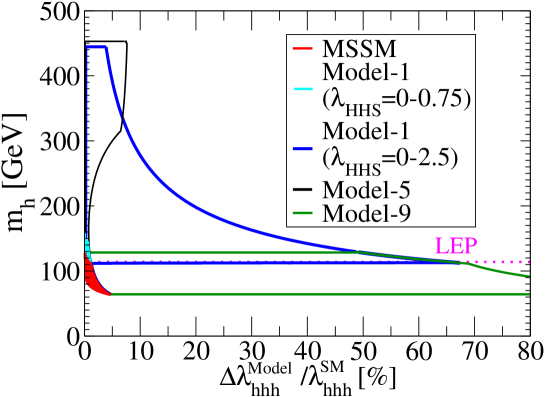
Figure 3: Possible allowed regions in the $m_{h}$-$(\Delta\lambda_{hhh}/\lambda_{hhh})$ plane in the MSSM, Model-1, Model-5 and Model-9 with scanned $\tan\beta$.

In Fig. 3, possible allowed regions with scanned $\tan\beta$ are shown in the $m_{h}$-$(\Delta\lambda_{hhh}^{\rm Model}/\lambda_{hhh}^{\rm SM})$ plane in Model-1, Model-5 and Model-9 as well as the MSSM. The maximal values of $\lambda_{HH\phi}$ in Model-1, Model-5 and Model-9 are taken to be the same as those in Fig. 2. The region in the MSSM (Model-1 with $0\lesssim\lambda_{HHS}\lesssim 0.75$, which corresponds to $\Lambda\simeq 10^{16}$ GeV ellwanger ) is indicated as the red-filled (cyan-filled) one. The possible allowed regions are different among the models so that the information of $m_{h}$ and $\Delta\lambda_{hhh}^{\rm Model}$ can be used to classify the SSMs.

V Discussion and Conclusion

We have studied $m_{h}$ and the $hhh$ coupling at the one-loop level in various SSMs, where $h$ is the lightest SM like Higgs boson. In a class of SSMs, the mass of the lightest Higgs boson, which is lower than 120-130 GeV in the MSSM, can be much higher due to the F-term contribution. Such an enhancement appears in the models with the extra neutral singlet or the triplet superfield. The upper bounds on $m_{h}$ are determined by the size of the coupling constants of the F-term, which can be constrained by the renormalization group equation analysis with an imposed cut-off scale $\Lambda$. Consequently, $m_{h}$ can be higher than 300-400 GeV when $\Lambda$ is at the TeV scale in Model-1 with small $\tan\beta$ values and Model-5.

Although the one-loop correction to the $hhh$ coupling due to the extra scalar components vanishes in the decoupling limit, it can be significant in particular SSMs such as Model-1 with large $\tan\beta$ and Model-9, when $\lambda_{HH\phi_{i}}^{2}v^{2}\sim M_{\phi_{i}}^{2}$ where $M_{\phi_{i}}$ is the invariant mass parameter of the extra field $\phi_{i}$ in the loop. In such a case, quartic powerlike mass contributions can appear as non-decoupling effects, and the correction can be larger than several times ten percent under the constraint from parturbativity. In this letter the analysis has been restricted in the effective potential method, where all the external momenta are set on zero. In the actual measurement of the $hhh$ coupling, one might think that the momentum dependences would be important. For example, at the LHC the $hhh$ coupling may be measured by $W$ fusion process $W^{+*}W^{-*}\rightarrow h^{*}\rightarrow hh$hhh_lhc , where the measured $hhh$ coupling is a function of $\sqrt{\hat{s}}$ the energy of the elementary process. At the ILC and its $\gamma\gamma$ option, the processes $e^{+}e^{-}\rightarrow Z^{\ast}\rightarrow Zh^{\ast}\rightarrow Zhh$hhh_lc and $\gamma\gamma\rightarrow h^{\ast}\rightarrow hh$gammagamma can be used. The energy dependence of the $hhh$ coupling has been discussed in Ref. KKOSY : see Fig. 3 in it. It is shown that unless $\sqrt{\hat{s}}\gg 2m_{h}$, the energy dependence is small in the bosonic loop contributions to the $hhh$ coupling . In addition, the non-decoupling effect in the wave function renormalization is at most quadratic instead of quartic in mass. Hence the wave function correction to the $hhh$ coupling is known to be as large as of order one percent and it is negligiblenondec . Consequently the calculation by using the effective potential gives a good approximation for our analysis.

In conclusion, even when only $h$ is observed in future, precision measurements of $m_{h}$ and the $hhh$ coupling can help discriminate the SSMs. Such discrimination can be improved if extra information for $\tan\beta$ can be used from, for example, future flavour experiments such as those for $B_{s}\rightarrow\mu\mu$, $B\rightarrow\tau\nu$ and so on.

In any case, the $hhh$ coupling is required to be measured with ${\cal O}(10)$ % accuracy, which may be expected at future colliders such as the LHC upgrade, the ILC and the CLIC hhh_lc .

- (1) The LEP Electroweak Working Group, http://lepewwg.web.cern.ch/LEPEWWG/
- (2) T. Aaltonen et al., Phys. Rev. Lett. 104, 061802 (2010).
- (3) A. Djouadi, W. Kilian, M. Muhlleitner and P. M. Zerwas, Eur. Phys. J. C 10, 45 (1999); U. Baur, T. Plehn and D. L. Rainwater, Phys. Rev. D 69, 053004 (2004); Phys. Rev. Lett. 89, 151801 (2002).
- (4) A. Djouadi, W. Kilian, M. Muhlleitner and P. M. Zerwas, Eur. Phys. J. C 10, 27 (1999); M. Battaglia, E. Boos and W. M. Yao, arXiv:hep-ph/0111276; Y. Yasui, et al., arXiv:hep-ph/0211047.
- (5) G. V. Jikia, Nucl. Phys. B 412, 57 (1994); R. Belusevic and G. Jikia, Phys. Rev. D 70, 073017 (2004) [arXiv:hep-ph/0403303].
- (6) Y. Okada, M. Yamaguchi and T. Yanagida, Prog. Theor. Phys. 85, 1 (1991); J. R. Ellis, G. Ridolfi and F. Zwirner, Phys. Lett. B 257, 83 (1991). H. E. Haber and R. Hempfling, Phys. Rev. Lett. 66, 1815 (1991).
- (7) J. R. Ellis, J. F. Gunion, H. E. Haber, L. Roszkowski and F. Zwirner, Phys. Rev. D 39, 844 (1989); M. Drees, Int. Jour. of Mod. Phys. A4, 3635 (1989); J. R. Espinosa and M. Quiros, Phys. Lett. B 279, 92 (1992).
- (8) T. Moroi and Y. Okada, Phys. Lett. B 295 73 (1992); U. Ellwanger, Phys. Lett. B 303, 271 (1993); G. L. Kane, C. F. Kolda and J. D. Wells, Phys. Rev. Lett. 70, 2686 (1993).
- (9) U. Ellwanger, C. Hugonie and A. M. Teixeira, arXiv:0910.1785 [hep-ph].
- (10) J. E. Kim and H. P. Nilles, Phys. Lett. B 138, 150 (1984).
- (11) J. R. Espinosa and M. Quiros, Phys. Rev. Lett. 81, 516 (1998).
- (12) P. Batra, A. Delgado, D. E. Kaplan and T. M. P. Tait, JHEP 0402, 043 (2004); R. Barbieri, E. Bertuzzo, M. Farina, P. Lodone and D. Pappadopulo, JHEP 1008, 024 (2010).
- (13) R. Harnik, G. D. Kribs, D. T. Larson and H. Murayama, Phys. Rev. D 70, 015002 (2004); S. Chang, C. Kilic and R. Mahbubani, Phys. Rev. D 71, 015003 (2005).
- (14) A. Zee, Phys. Lett. B 93, 389 (1980) [Erratum-ibid. B 95, 461 (1980)]; Phys. Lett. B 161, 141 (1985); Nucl. Phys. B 264, 99 (1986); K. S. Babu, Phys. Lett. B 203, 132 (1988); L. M. Krauss, S. Nasri and M. Trodden, Phys. Rev. D 67, 085002 (2003); M. Aoki, S. Kanemura and O. Seto, Phys. Rev. Lett. 102, 051805 (2009). M. Aoki, S. Kanemura, T. Shindou and K. Yagyu, JHEP 1007, 084 (2010).
- (15) R. Barbieri, L. J. Hall and V. S. Rychkov, Phys. Rev. D 74, 015007 (2006); E. Ma, Phys. Rev. D 73, 077301 (2006); J. Kubo, E. Ma and D. Suematsu, Phys. Lett. B 642, 18 (2006).
- (16) J. C. Pati and A. Salam, Phys. Rev. D 10, 275 (1974) [Erratum-ibid. D 11, 703 (1975)]; R. N. Mohapatra and J. C. Pati, Phys. Rev. D 11, 2558 (1975); G. Senjanovic and R. N. Mohapatra, Phys. Rev. D 12, 1502 (1975).
- (17) T. P. Cheng and L. F. Li, Phys. Rev. D 22, 2860 (1980); J. Schechter and J. W. F. Valle, Phys. Rev. D 22, 2227 (1980); A. Rossi, Phys. Rev. D 66, 075003 (2002).
- (18) S. R. Coleman and E. J. Weinberg, Phys. Rev. D 7, 1888 (1973).
- (19) J. R. Espinosa and M. Quiros, Phys. Lett. B 266, 389 (1991); R. Hempfling and A. H. Hoang, Phys. Lett. B 331, 99 (1994); M. S. Carena, M. Quiros and C. E. M. Wagner, Nucl. Phys. B 461, 407 (1996).
- (20) S. P. Martin, Phys. Rev. D 67, 095012 (2003); G. Degrassi, S. Heinemeyer, W. Hollik, P. Slavich and G. Weiglein, Eur. Phys. J. C 28, 133 (2003); B. C. Allanach, A. Djouadi, J. L. Kneur, W. Porod and P. Slavich, JHEP 0409, 044 (2004).
- (21) S. Kanemura, T. Shindou, and K. Yagyu, in preparation.
- (22) N. Cabibbo, L. Maiani, G. Parisi and R. Petronzio, Nucl. Phys. B 158, 295 (1979).
- (23) S. Kanemura, S. Kiyoura, Y. Okada, E. Senaha and C. P. Yuan, Phys. Lett. B 558, 157 (2003).
- (24) S. Kanemura, Y. Okada, E. Senaha and C. P. Yuan, Phys. Rev. D 70, 115002 (2004).
- (25) T. Appelquist and J. Carazzone, Phys. Rev. D 11, 2856 (1975).
- (26) S. Kanemura, T. Kubota and E. Takasugi, Phys. Lett. B 313, 155 (1993); A. G. Akeroyd, A. Arhrib and E. M. Naimi, Phys. Lett. B 490, 119 (2000); I. F. Ginzburg and I. P. Ivanov, Phys. Rev. D 72, 115010 (2005).
- (27) S. Kanemura, Y. Okada and E. Senaha, Phys. Lett. B 606, 361 (2005).
- (28) A. G. Cohen, D. B. Kaplan and A. E. Nelson, Phys. Lett. B 245, 561 (1990); Ann. Rev. Nucl. Part. Sci. 43, 27 (1993).
- (29) E. Asakawa, D. Harada, S. Kanemura, Y. Okada and K. Tsumura, Phys. Lett. B 672, 354 (2009) [arXiv:0809.0094 [hep-ph]].