Abstract. We study nongeneric planar trees and prove the existence of a Gibbs measure on infinite trees obtained as a weak limit of the finite volume measures. It is shown that in the infinite volume limit there arises exactly one vertex of infinite degree and the rest of the tree is distributed like a subcritical Galton-Watson tree with mean offspring probability $m<1$. We calculate the rate of divergence of the degree of the highest order vertex of finite trees in the thermodynamic limit and show it goes like $(1-m)N$ where $N$ is the size of the tree. These trees have infinite spectral dimension with probability one but the spectral dimension calculated from the ensemble average of the generating function for return probabilities is given by $2\beta-2$ if the weight $w_{n}$ of a vertex of degree $n$ is asymptotic to $n^{-\beta}$.

1 Introduction

In the recent past the interest of scientists in various classes of random graphs and networks has increased dramatically due to the many applications of these mathematical structures to describe objects and relationships in subjects ranging from pure mathematics and computer science to physics, chemistry and biology. An important class of graphs in this context are tree graphs, both because many naturally appearing random graphs are trees and also because trees are analytically more tractable than general graphs and one expects that some features of general random graphs can be understood by looking first at trees.

In this paper we study an equilibrium statistical mechanical model of planar trees. The parameters of the model are given by a sequence of non–negative numbers $(w_{i})_{i\geq 1}$, referred to as branching weights. To a finite tree $\tau$ we assign a Boltzmann weight

$$W(\tau)=\prod_{i\in V(\tau)}w_{\sigma_{i}}$$

where $V(\tau)$ is the vertex set of $\tau$ and $\sigma_{i}$ is the degree of the vertex $i$. The model is local, in the sense that the energy of a tree is given by the sum over the energies of individual vertices. In [7] the critical exponents of this model were calculated and its phase structure was described. It was argued that the model exhibits two phases in the thermodynamic limit: a fluid (elongated, generic) phase where the trees are of a large diameter and have vertices of finite degree and a condensed (crumpled) phase where the trees are short and bushy with exactly one vertex of infinite degree.

A complete characterization of the fluid phase, referred to as generic trees, was given in [17, 20] where it was shown that the Gibbs measures converge to a measure concentrated on the set of trees with exactly one non–backtracking path from the root to infinity having critical Galton-Watson outgrowths. In [20] it was furthermore proved that the trees have Hausdorff dimension $d_{H}=2$ and spectral dimension $d_{s}=4/3$ with respect to the infinite volume measure. The purpose of this paper is to establish analogous results for the condensed phase. Preliminary results in this direction were obtained in [31].

One of the motivations for the study of the tree model is that a similar phase structure is seen for more general class of graphs in models of simplicial gravity [1, 2]. In these models the elongated phase seems to be effectively described by trees [3] and it has been established by numerical methods that in the condensed phase a single large simplex appears whose size increases linearly with the graph volume [15, 24]. In [12] it was proposed that the same mechanism is behind the phase transition in the different models and the so called constrained mean field model was introduced in order to capture this feature. This idea was developed in a series of papers [6, 8, 9, 10, 11] where the model was studied under the name “balls in boxes” or “backgammon model”. The model consists of placing $N$ balls into $M$ boxes and assigning a weight to each box depending only on the number of balls it contains. In [9] the critical exponents were calculated and the two phases characterized. The distribution of the box occupancy number was derived and it was argued that in the condensed phase exactly one box contains a large number of balls which increases linearly with the system size.

A model equivelant to the “balls in boxes” model was studied in a recent paper [27]. It is an equilibrium statistical mechanical model with a local action of the form described above but the class of trees is restricted to so called caterpillar graphs. Caterpillars are trees which have the property that if all vertices of degree one and the edges containing them are removed, the resulting graph is linear. The caterpillar model was solved by proving convergence of the Gibbs measures to a measure on infinite graphs and the limiting measure was completely characterized. It was shown that in the fluid phase the measure is concentrated on the set of caterpillars of infinite length and that in the condensed phase it is concentrated on the set of caterpillars which are of finite length and have precisely one vertex of infinite degree. This was the first rigourous treatment of the condensed phase in models of the above type. A model of random combs, equivalent to the caterpillar model was studied in [18] where analagous results were obtained for the limiting measure. A closely related phenomenom of condensation also appears in dynamical systems such as the zero range process, see e.g. [21].

In this paper we use techniques similar to those of [27] with some additional input from probability theory to prove convergence of the Gibbs measures in the condensed phase of the planar tree model. In Section 2 we generalize the definition of planar trees to allow for vertices of infinite degree and define a metric on the set of planar trees which has the nice properties that the metric space is compact and that the subset of finite trees is dense. In Section 3 we recall the definition of generic and nongeneric trees, define the partition functions of interest and recall the relation to Galton-Watson processes. Section 4 is the technical core of the paper. There we review some results we need from probability theory and then show that the partition function $Z_{N}$ for nongeneric trees of size $N$ has the asymptotic behavior

$$Z_{N}\sim N^{-\beta}\zeta_{0}^{-N}$$ (1.1)

where $\zeta_{0}$ is a constant and $\beta$ is the exponent of the power decay of the weight $w_{n}$ of vertices of degree $n$, i.e. $w_{n}\sim n^{-\beta}$. In Section 5 we establish the existence of the infinite volume Gibbs measure and prove that in the condensed phase it is concentrated on the set of trees of finite diameter with precisely one vertex of infinite degree and that the rest of the tree is distributed as a subcritical Galton-Watson process with mean offspring probability $m<1$. We prove that for finite trees the degree of the large vertex grows linearly with the system size $N$ as $(1-m)N$ with high probability, confirming the result stated in [14]. We conclude in Section 6 by calculating the annealed spectral dimension of the trees in the condensed phase. In [16] it was claimed, on the basis of scaling arguments, that the spectral dimension is $d_{s}=2$. We prove, however, that if the spectral dimension exists it is given by $d_{s}=2\beta-2$. In fact, it takes the same value as the spectral dimension of the condensed phase in the caterpillar model [27].

2 Rooted planar trees

In this section we recall the definition of rooted planar trees and define a convenient metric on the set of all such trees. We establish some elementary properties of the trees as a metric space which will be needed in the construction of a measure on infinite trees. The combinatorial definition of planar trees below is in the spirit of [17] with the change that we allow for vertices of infinite degree. We require this extension since vertices of infinite degree appear in the thermodynamic limit in the nongeneric phase of the random tree model in Section 4.

The planarity condition means that links incident on a vertex are cyclically ordered. When the degree of a vertex is infinite there are nontrivial different possibilities of ordering the links and therefore the planarity condition must by carefully defined. We allow vertices of at most countably infinite degree and the edges are given the simplest possible ordering, i.e. if we look at the set of edges leading away from the root at a given vertex, then the smallest edge is the leftmost one which is required to exist and the remaining edges are ordered as $\mathbb{N}$. Note that we could just as well choose the rightmost edge as the smallest and order the remaining ones counterclockwise as $\mathbb{N}$. The root will always be taken to have order one for convenience but this is not an essential assumption.

Let $(D_{R})_{R\geq 0}$ be a sequence of pairwise disjoint, countable sets with the properties that if $D_{R}=\emptyset$ then $D_{r}=\emptyset$ for all $r\geq R$. The sets $D_{0}$ and $D_{1}$ are defined to have only a single element. The set $D_{R}$ will eventually denote the set of vertices at graph distance $R$ from the root. We will denote the number of elements in a set $A$ by $|A|$. To introduce the edges and the planarity condition, we define orderings on each of the sets $D_{R}$ and order preserving maps

$$\phi_{R}:D_{R}\longrightarrow D_{R-1},\quad\quad R\geq 1$$ (2.1)

which satisfy the following: For each vertex $v\in D_{R-1}$ such that
$|\phi^{-1}_{R}(v)|=\infty$, there exists an order preserving isomorphism

$$\psi_{v}:\mathbb{N}\longrightarrow\phi^{-1}_{R}(v).$$ (2.2)

In this notation $\phi_{R}(w)$ is the parent of the vertex $w$ and $|\phi^{-1}_{R}(v)|+1$ is the degree of the vertex $v$, denoted $\sigma_{v}$. One can show by induction on $R$ that such orderings on the sets $D_{R}$ can be defined and that they are well orderings, i.e. each subset of $D_{R}$ has a smallest element. It is not hard to check that given the ordered sets $D_{R},R\geq 0$, and the order preserving maps $\phi_{R},R\geq 1$ with the above properties the maps $\psi_{v}$ are unique. For a vertex $v$ of a finite degree we can also define the mappings $\psi_{v}$ and they are trivial.

Let $\tilde{\Gamma}$ be the set of all pairs of sequences $\{(D_{0},D_{1},D_{2},\ldots),(\phi_{1},\phi_{2},\ldots)\}$ which satisfy the above conditions. We define an equivalence relation $\sim$ on $\tilde{\Gamma}$ by

$$\{(D_{0},D_{1},\ldots),(\phi_{1},\phi_{2},\ldots)\}\sim\{(D^{\prime}_{0},D^{\prime}_{1},\ldots),(\phi^{\prime}_{1},\phi^{\prime}_{2},\ldots)\}$$ (2.3)

if and only if for all $R\geq 1$ there exist order isomorphisms $\chi_{R}:D_{R}\longrightarrow D^{\prime}_{R}$ such that $\phi^{\prime}_{R}=\chi_{R-1}\circ\phi_{R}\circ\chi_{R}^{-1}$. Note that since the sets $D_{R}$ are well ordered for all $R\geq 1$ the order isomorphisms $\chi_{R}$ are unique. Define $\Gamma=\tilde{\Gamma}/\sim$. If $\tau\in\tilde{\Gamma}$ we denote the equivalence class of $\tau$ by $[\tau]$ and call it a rooted planar tree. As a graph, the tree has a vertex set

$$V=\bigcup_{R=0}^{\infty}D_{R}$$ (2.4)

and an edge set

$$E=\{(v,\phi_{R}(v))~{}|~{}v\in D_{R},R\geq 1\}$$ (2.5)

which are independent of the representative $\{(D_{0},D_{1},\ldots),(\phi_{1},\phi_{2},\ldots)\}$ up to graph isomorphisms. The single element in $D_{0}$ is called the root and denoted by $r$. We denote the set of all rooted planar trees on $N$ edges by $\Gamma_{N}$ and the set of finite rooted planar trees by $\Gamma^{\prime}=\bigcup_{N=1}^{\infty}\Gamma_{N}$.

In the following, all properties of trees $[\tau]\in\Gamma$ that we are interested in are independent of representatives and we write $\tau$ instead of $[\tau]$. We then write $D_{R}(\tau)$, $\phi_{R}(\cdot,\tau)$, $\psi_{v}(\cdot,\tau)$, $\sigma_{v}(\tau)$ etc. when we need the more detailed information on $\tau$. If it is clear which tree we are working with we skip the argument $\tau$. When we draw the trees in the plane we use the convention that $\psi_{v}(k)$ is the $k$-th vertex clockwise from the nearest neighbour of $v$ closest to the root, see Figure 1.

Figure 1: The ordering of $\phi^{-1}_{R}(v)$.

For a tree $\tau\in\Gamma$ we denote its height, i.e. the maximal graph distance of its vertices from the root, by $h(\tau)$. For a pair of vertices $v$ and $w$ we denote the unique shortest path from $v$ to $w$ by $(v,w)$. The ball of radius $R$, $B_{R}(\tau)$ is defined as the subtree of $\tau$ generated by $D_{0}(\tau),D_{1}(\tau)\ldots D_{R}(\tau)$.

We define the left ball of radius $R$, $L_{R}(\tau)$, as the subtree of $B_{R}(\tau)$ generated by subsets $E_{S}\subseteq D_{S}(B_{R}(\tau))$, $S=0,...R$, such that $E_{0}=D_{0}(B_{R}(\tau))$, $E_{1}=D_{1}(B_{R}(\tau))$ and

$$E_{S}=\{\psi_{v}(i)~{}|~{}v\in E_{S-1},i=1,2,\ldots,\min\{R,\sigma_{v}\}-1\},$$ (2.6)

see Fig. 2. We denote the number of edges in a tree $\tau$ by $|\tau|$. It is easy to check that for all $\tau\in\Gamma$

$$|L_{R}(\tau)|\leq{\frac{(R-1)^{R}-1}{R-2}},$$ (2.7)

whereas the number of elements in $B_{R}(\tau)$ can be infinite.

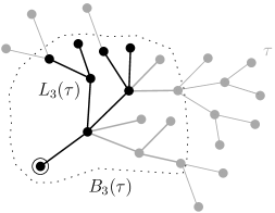
Figure 2: An example of the subgraphs $B_{R}(\tau)$ and $L_{R}(\tau)$.

We define a metric $d$ on $\Gamma$ by

$$d(\tau,\tau^{\prime})=\min\left\{\left.\frac{1}{R}~{}\right|~{}L_{R}(\tau)=L_{R}(\tau^{\prime}),~{}R\in\mathbb{N}\right\},\quad\quad\tau,\tau^{\prime}\in\Gamma.$$ (2.8)

It is elementary to check that this is in fact a metric. Note that if we allow any ordering on the infinite sets $|\phi^{-1}_{R}(v)|$, but still insist that they have a smallest element, then this ordering is in general not a a well ordering and $d$ is only a pseudometric.

Denote the open ball in $\Gamma$ centered at $\tau_{0}$ and with radius $r$ by

$$\mathcal{B}_{r}(\tau_{0})=\{\tau\in\Gamma~{}|~{}d(\tau_{0},\tau)<r\}.$$ (2.9)

Proposition 2.1

For $r>0$ and $\tau_{0}\in\Gamma$, the ball $\mathcal{B}_{r}(\tau_{0})$ is both open and closed and if $\tau_{1}\in\mathcal{B}_{r}(\tau_{0})$ then $\mathcal{B}_{r}(\tau_{1})=\mathcal{B}_{r}(\tau_{0})$.

• It is easy to see that open balls are also closed since the possible positive values of $d$ form a discrete set. To prove the second statement take a ball $\mathcal{B}_{r}(\tau_{0})$ and a tree $\tau_{1}\in\mathcal{B}_{r}(\tau_{0})$. First take an element $\tau_{2}\in\mathcal{B}_{r}(\tau_{1})$. We know that $L_{R}(\tau_{1})=L_{R}(\tau_{0})$ and $L_{R}(\tau_{1})=L_{R}(\tau_{2})$ for all $R<1/r$ so obviously $L_{R}(\tau_{0})=L_{R}(\tau_{2})$ for all $R<1/r$. Therefore

  $$d(\tau_{2},\tau_{0}) \leq \min\left\{\left.\frac{1}{R}~{}\right|~{}L_{R}(\tau_{2})=L_{R}(\tau_{0}),~{}R<1/r+1\right\}$$ (2.10)

  $$= \frac{1}{\lfloor 1/r+1\rfloor}<r.$$

  Therefore $\tau_{2}\in\mathcal{B}_{r}(\tau_{0})$ and thus $\mathcal{B}_{r}(\tau_{1})\subseteq\mathcal{B}_{r}(\tau_{0})$. With exactly the same argument we see that $\mathcal{B}_{r}(\tau_{0})\subseteq\mathcal{B}_{r}(\tau_{1})$ and therefore the equality is established.

  $\square$

Proposition 2.2

The metric space $(\Gamma,d)$ is compact and the set $\Gamma^{\prime}$ of finite trees is a countable dense subset of $\Gamma$.

• To prove compactness it is enough to note that by (2.7), for each $R\in\mathbb{N}$, the set $\{L_{R}(\tau)~{}|~{}\tau\in\Gamma\}$ is finite. The result then follows by the same arguments applied to the set of random walks in [17].

  In order to prove the density of $\Gamma^{\prime}$ we note that the sequence $\left(L_{n}(\tau)\right)_{n\in\mathbb{N}}$ is in $\Gamma^{\prime}$ by (2.7) and clearly converges to $\tau$.

  $\square$

3 Generic and nongeneric trees

In this section we define the tree ensemble that we study and discuss some of its elementary properties. Let $w_{n}$, $n\geq 1$ be a sequence of non–negative numbers which we call branching weights. For technical convenience we will always take

$$w_{1},w_{2}>0\quad\quad\text{and}\quad\quad w_{n}>0\quad\quad\text{for some $n\geq 3$}.$$ (3.1)

Let $V(\tau)$ be the set of vertices in $\tau$. The finite volume partition function is defined as

$$Z_{N}=\sum_{\tau\in\Gamma_{N}}~{}\prod_{i\in V(\tau)\setminus\{r\}}w_{\sigma_{i}}$$ (3.2)

where $\sigma_{i}$ is the degree of vertex $i$. We define a probability distribution $\nu_{N}$ on $\Gamma_{N}$ by

$$\nu_{N}(\tau)=Z_{N}^{-1}\prod_{i\in V(\tau)\setminus\{r\}}w_{\sigma_{i}}.$$ (3.3)

The weights $w_{n}$, or alternatively the measures $\nu_{N}$, define a tree ensemble. Note that $\nu_{N}$ is not affected by a rescaling of the branching weights of the form $w_{n}\rightarrow w_{n}ab^{n}$ where $a,b>0$. We introduce the generating functions

$$\mathcal{Z}(\zeta)=\sum_{N=1}^{\infty}Z_{N}\zeta^{N}$$ (3.4)

and

$$g(z)=\sum_{n=0}^{\infty}w_{n+1}z^{n}.$$ (3.5)

Then we have the standard relation

$$\mathcal{Z}(\zeta)=\zeta g(\mathcal{Z}(\zeta))$$ (3.6)

which is explained in Fig. 3.

Figure 3: A diagram explaining the recursion (3.6). The root is indicated by a circled point.

We denote the radius of convergence of $\mathcal{Z}(\zeta)$ and $g(z)$ by $\zeta_{0}$ and $\rho$, respectively, and define $\mathcal{Z}_{0}=\mathcal{Z}(\zeta_{0})$. If $\mathcal{Z}_{0}<\rho$, then by definition we have a generic ensemble of trees [20]. Otherwise we say that we have a nongeneric ensemble. If $\rho=\infty$ we always have a generic ensemble. If $\rho$ is finite we can assume that $\rho=1$ by scaling the branching weights $w_{n}\rightarrow w_{n}\rho^{n-1}$.

There is a useful relation between the tree ensemble $(\Gamma_{N},\nu_{N})$ and Galton–Watson (GW) trees (see e.g. [23]). Let $p_{n}$, $n=0,1,2\ldots$, be the offspring probability distribution for a GW tree. Then we link a vertex of order one (the root) to the ancestor of the GW tree and obtain a rooted tree with a root of degree 1. The GW process gives rise to a probability measure on the set of all finite trees

$$\mu(\tau)=\prod_{i\in V(\tau)\setminus\{r\}}p_{\sigma_{i}-1},\quad\quad\quad\text{where}\quad\quad\tau\in\Gamma^{\prime}.$$ (3.7)

Let $m$ be the average number of offsprings in the GW process. If $m>1$ the process is said to be supercritical and the probability that it survives forever is positive. If $m=1$ the process is said to be critical and it dies out with probability one. If $m<1$ the process is said to be subcritical and it dies out exponentially fast [23].

The probability distribution $\nu_{N}$ can be obtained from a GW process with offspring probabilities

$$p_{n}=\zeta_{0}w_{n+1}\mathcal{Z}_{0}^{n-1}$$ (3.8)

by conditioning the trees to be of size $N$

$$\nu_{N}(\tau)=\frac{\mu(\tau)}{\mu(\Gamma_{N})}.$$ (3.9)

The mean offspring probability is then

$$m=\mathcal{Z}_{0}\frac{g^{\prime}(\mathcal{Z}_{0})}{g(\mathcal{Z}_{0})}.$$ (3.10)

Generic trees always correspond to critical GW processes [20] and nongeneric trees can correspond to either critical or subcritical GW processes. In all cases $m\leq 1$. We now analyze this in more detail.

Fix a set of branching weights $w_{n}$ which give $\rho=1$ but let $w_{1}$ be a free parameter of the model which at this stage can be either generic or nongeneric. Define

$$h(\mathcal{Z})=\frac{g(\mathcal{Z})}{\mathcal{Z}}.$$ (3.11)

From (3.6) we see that $h(\mathcal{Z})=1/\zeta(\mathcal{Z})$ for $\mathcal{Z}\leq\mathcal{Z}_{0}$. Differentiating $h$ we get

$$h^{\prime}(\mathcal{Z})=\frac{g(\mathcal{Z})}{\mathcal{Z}^{2}}\left[\mathcal{Z}\frac{g^{\prime}(\mathcal{Z})}{g(\mathcal{Z})}-1\right]$$ (3.12)

and again

$$h^{\prime\prime}(\mathcal{Z})=\frac{g^{\prime\prime}(\mathcal{Z})}{\mathcal{Z}}-\frac{2}{\mathcal{Z}}h^{\prime}(\mathcal{Z}).$$ (3.13)

The genericity condition means that $h$ has a quadratic minimum at $\mathcal{Z}=\mathcal{Z}_{0}<1$, see Fig. 4. It follows that $m=1$, showing that the generic phase corresponds to critical GW trees. Furthermore, given $\mathcal{Z}_{0}<1$ and the branching weights $w_{n}$, $n\geq 2$, we have $w_{1}=\sum_{n=2}^{\infty}(n-2)w_{n}\mathcal{Z}_{0}^{n-1}$. We can therefore clearly make any model with $\rho=1$ generic by choosing

$$w_{1}<\sum_{n=2}^{\infty}(n-2)w_{n}\equiv w_{c}.$$ (3.14)

Here $w_{c}$ is a critical value for $w_{1}$ which depends on $w_{n}$ for $n\geq 3$. We note that if $w_{c}=\infty$, i.e. if $g^{\prime}(z)$ diverges as $z\rightarrow 1$, we always have a generic ensemble.

Figure 4: The three possible scenarios. a) Generic, critical, $w_{1}<w_{c}$.
b) nongeneric, critical, $w_{1}=w_{c}$. c) nongeneric, subcritical, $w_{1}>w_{c}$.

The next possible scenario is that $h$ has a quadratic minimum at $\mathcal{Z}=\mathcal{Z}_{0}=1$. This happens when $w_{1}=w_{c}$ or in other words when $m=1$. This is a nongeneric ensemble which still corresponds to critical GW trees.

Finally, by choosing $w_{1}>w_{c}$, $h$ has no quadratic minimum and $m<1$. In this case the trees are nongeneric and correspond to subcritical GW trees as we will explore in detail in the next section.

4 Subcritical nongeneric trees

In this section we examine the subcritical nongeneric phase and determine the asymptotic behaviour of $Z_{N}$. This will allow us to construct the infinite volume Gibbs measure in the next section.

We fix a number $\beta\geq 0$ and for $n\geq 2$ we choose the branching weights such that

$$w_{n}=n^{-\beta}(1+o(1)),\quad n\geq 2$$ (4.1)

and let $w_{1}$ be a free parameter. In this case $\rho=1$. If $\beta\leq 2$ then $g^{\prime}(1)=\infty$ and therefore we have the generic phase for all values of $w_{1}$. If $\beta>2$ we can have any one of the three cases discussed in the previous section depending on the value of $w_{1}$, see Fig. 5.

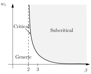
Figure 5: A diagram showing the possible phases of the trees. The critical line is determined by the equation $w_{1}=w_{c}$.

Now choose $\beta>2$ and $w_{1}>w_{c}$ such that

$$m=\frac{g^{\prime}(1)}{g(1)}<1$$ (4.2)

so we are in the nongeneric, subcritical phase. Then $\mathcal{Z}_{0}=\rho=1$ and we see from (3.6) that

$$\zeta_{0}=\frac{1}{g(1)}.$$ (4.3)

The main result of this section is the following.

Theorem 4.1

If the branching weights (4.1) satisfy (4.2) then the partition function has the asymptotic behaviour

$$Z_{N}=(1-m)^{-\beta}N^{-\beta}\zeta_{0}^{1-N}\left(1+o(1)\right).$$ (4.4)

The remainder of this section is devoted to a proof of this theorem. To determine the large $N$ behaviour of $Z_{N}$ we split it into two parts,

$$Z_{N}=Z_{1,N}+E_{N},$$ (4.5)

where $Z_{1,N}$ is the contribution to $Z_{N}$ from trees which have exactly $1$ vertex of maximal degree and $E_{N}$ is the contribution to $Z_{N}$ from trees which have $\geq$ 2 vertices of maximal degree. We will estimate these two terms seperately and show that for large $N$ the main contribution comes from $Z_{1,N}$. It follows from the proof that large trees, of size $N$, are most likely to have exactly one large vertex which is approximately of degree $(1-m)N$. This will be stated more precisely in Section 5. The arguments used in the proof of Theorem 4.1 rely on a “truncation method” and some classical results from probability theory. We begin the proof by defining truncated versions of the generating functions introduced in the previous section. Then we introduce some notation and terminology from probability theory and state a few lemmas. In Subsection 4.2 we analyse the asymptotic behaviour of $Z_{1,N}$ and in Subsection 4.3 we do the same for $E_{N}$.

For the truncation method, we will need the following definitions. Let $L_{i,N}$ be the finite volume partition function for trees on $N$ edges which have all vertices of degree $\leq i$ and define the generating functions

$$\mathcal{L}_{i}(\zeta)=\sum_{N=1}^{\infty}L_{i,N}\zeta^{N}$$ (4.6)

and

$$\ell_{i}(z)=\sum_{n=0}^{i-1}w_{n+1}z^{n}.$$ (4.7)

We have the standard relation

$$\mathcal{L}_{i}(\zeta)=\zeta\ell_{i}(\mathcal{L}_{i}(\zeta))$$ (4.8)

obtained in the same way as (3.6). Let $Y_{j,i,N}$ be the finite volume partition function for trees on $N$ edges which have all vertices of degree $\leq i$ and one marked (but not weighted) vertex of degree one at distance $j$ from the root. Define

$$\mathcal{Y}_{j,i}(\zeta)=\sum_{N=1}^{\infty}Y_{j,i,N}\zeta^{N}$$ (4.9)

and

$$\mathcal{Y}_{i}(\zeta)=\sum_{j=1}^{\infty}\mathcal{Y}_{j,i}(\zeta).$$ (4.10)

With generating function arguments we find that

$$\mathcal{Y}_{j,i}(\zeta)=\zeta\ell_{i}^{\prime}(\mathcal{L}_{i}(\zeta))\mathcal{Y}_{j-1,i}(\zeta)$$ (4.11)

for $j\geq 2$, see Fig. 6. Using $\mathcal{Y}_{1,i}(\zeta)=\zeta$ this yields by induction

$$\mathcal{Y}_{j,i}(\zeta)=\zeta\Big{(}\zeta\ell_{i}^{\prime}(\mathcal{L}_{i}(\zeta))\Big{)}^{j-1}.$$ (4.12)

Figure 6: A diagram explaining (4.11). The marked vertex is indicated by $\otimes$. The balloons containing “$\leq i$” are trees which have vertices of degree at most $i$. If the degree of the nearest neighbour to the root is $k+1$, there are $k$ different ways of placing the marked vertex in a balloon.

Summing over $j$ we get

$$\mathcal{Y}_{i}(\zeta)=\frac{\zeta}{1-\zeta\ell_{i}^{\prime}(\mathcal{L}_{i}(\zeta))}.$$ (4.13)

4.1 Tools from probability theory

It will be useful to formulate our problem in probabilistic language. Define the probability generating functions

$$f_{i}(z)=\frac{\ell_{i}(z)}{\ell_{i}(1)}\quad\quad\text{and}\quad\quad f(z)=\frac{g(z)}{g(1)}.$$ (4.14)

If $A$ is an event, we let $\mathbb{P}(A)$ denote the probability of $A$. Let $X^{(i)}_{1},X^{(i)}_{2},\ldots$ be i.i.d. random variables which have a probability generating function $f_{i}(z)$, i.e.

$$\mathbb{P}(X^{(i)}_{j}=k)=\left\{\begin{array}[]{ll}w_{k+1}/\ell_{i}(1)&\text{if $0\leq k\leq i-1$},\\ 0&\text{if $k>i-1,$}\end{array}\right.$$ (4.15)

and let $X_{1},X_{2},\ldots$ be i.i.d. random variables which have a probability generating function $f(z)$. Define

$$m_{i}=\mathbb{E}(X^{(i)}_{j}),\quad V_{i}=\text{Var}(X^{(i)}_{j}),\quad\quad S^{(i)}_{N}=X^{(i)}_{1}+\ldots+X^{(i)}_{N}$$ (4.16)

and

$$\quad\quad S_{N}=X_{1}+\ldots+X_{N}.$$ (4.17)

Note that $m=\mathbb{E}(X_{j})$ and from (4.2) we know that $m<1$. Clearly $m_{i}\longrightarrow m$ as $i\longrightarrow\infty$. We need now a few lemmas, the first three deal with convergence rates in the weak law of large numbers.

Lemma 4.2

For any $\epsilon>0$ and any $s<\beta-2$ we have

$$\lim_{N\rightarrow\infty}N^{s}\mathbb{P}\left(\left|\frac{S_{N}}{N}-m\right|>\epsilon\right)=0.$$ (4.18)

• It is clear that $\mathbb{E}(|X_{j}|^{t})<\infty$ for all $t<\beta-1$ and the same is true for the translated random variables $X_{j}-m$. The result then follows directly from [29, Theorem 28, p. 286].

  $\square$

The next Lemma is a classical result [5].

Lemma 4.3

(Bennett’s inequality) If $W_{1},W_{2},\ldots$ are independent random variables, $\mathbb{E}(W_{j})=0$, $\mathrm{Var}(W_{j})=V_{W}$ and $W_{j}\leq b$ a.s. for every $j$, where $b$ and $V_{W}$ are positive numbers, then for any $\epsilon>0$

$$\mathbb{P}\left(\frac{1}{N}\sum_{j=1}^{N}W_{j}>\epsilon\right)\leq\exp\left\{-\eta\left[\left(1+\frac{1}{\lambda}\right)\log\left(1+\lambda\right)-1\right]\right\}$$ (4.19)

with

$$\eta=\frac{N\epsilon}{b}\quad\quad\text{and}\quad\quad\lambda=\frac{b\epsilon}{V_{W}}.$$ (4.20)

By $f(x)=\Theta(g(x))$ as $x\rightarrow\infty$ we mean that for $x$ sufficiently large, there exist constants $c_{1}$ and $c_{2}$ such that $c_{1}g(x)\leq f(x)\leq c_{2}g(x)$.

Lemma 4.4

If $i=\Theta(N^{\gamma})$ where $\gamma<1$ then, for any $\epsilon>0$ small enough, there is a positive constant $C$ such that

$$\mathbb{P}\left(\frac{S^{(i)}_{N}}{N}-m_{i}>\epsilon\right)\leq\exp\left\{-C\epsilon N^{1-\gamma}\right\}.$$ (4.21)

• This follows directly from Bennett’s inequality with $W_{j}=X^{(i)}_{j}-m_{i}$. Then $V_{W}=V_{i}$ and we can take $b=i$ for $i$ large enough (since $m_{i}<1$ for $i$ large enough). If now $i=\Theta(N^{\gamma})$, then

  $$\eta=\epsilon\Theta(N^{1-\gamma}).$$ (4.22)

  If $\beta>3$ then $V_{i}<\infty$ and $\lambda=\Theta(N^{\gamma})$ and the result follows. If $2<\beta\leq 3$ then

  $$V_{i}=\left\{\begin{array}[]{ll}\Theta(i^{3-\beta})&\text{if $\beta<3$},\\ \Theta(\log(i))&\text{if $\beta=3$}\end{array}\right.$$ (4.23)

  so $\lambda\longrightarrow\infty$ as $N\longrightarrow\infty$ which completes the proof.

  $\square$

In the following we will repeatedly use Lagrange’s inversion formula, see e.g. [32, p. 167]. We denote the coefficient of $z^{n}$ in a formal power series $p(z)$ by $[z^{n}]\left\{p(z)\right\}$.

Lemma 4.5

(Lagrange’s inversion formula) If $h(z)$ is a formal power series in $z$ and $\mathcal{L}_{i}$ satisfies (4.8) then

$$[\zeta^{N}]\left\{h(\mathcal{L}_{i}(\zeta))\right\}=\frac{1}{N}[z^{N-1}]\left\{h^{\prime}(z)\ell_{i}(z)^{N}\right\}.$$ (4.24)

Using the above Lemma for the function $h(z)=z^{j}$ we get

$$[\zeta^{N}]\left\{\mathcal{L}_{i}(\zeta)^{j}\right\}=\frac{j}{N}[z^{N-j}]\left\{\ell_{i}(z)^{N}\right\}.$$ (4.25)

The following simple result will be useful. We omit the proof.

Lemma 4.6

If $X\geq 0$ and $Y$ are random variables, then for any $\epsilon>0$

$$\mathbb{P}\left(\left|X+Y\right|\leq\epsilon\right)\geq\mathbb{P}\left(X\leq\epsilon/2\right)\mathbb{P}\left(\left|Y\right|\leq\epsilon/2\right)$$ (4.26)

and

$$\mathbb{P}\left(\left|X+Y\right|>\epsilon\right)\leq\mathbb{P}\left(\left|Y\right|>\epsilon/2\right)+\mathbb{P}\left(X>\epsilon/2\right).$$ (4.27)

4.2 Calculation of $Z_{1,N}$

Using the Lemmas in the previous subsection we are ready to study the asymptotic behaviour of $Z_{1,N}$. It is is easy to see that

$$Z_{1,N} = \sum_{i=0}^{N-1}w_{i+1}[\zeta^{N}]\left\{\mathcal{Y}_{i}(\zeta)\mathcal{L}_{i}(\zeta)^{i}\right\}$$ (4.28)

as is illustrated in Fig. 7.

Figure 7: An illustration of Equation (4.28). The balloons which include the “$\leq i$” are trees which have vertices of degree at most $i$. There is thus precisely one vertex of maximum degree $i+1$.

Combining (4.8) and (4.13) one can use the Lagrange inversion formula (4.24) for the function

$$h_{ij}(z)=\frac{z^{j+1}}{\ell_{i}(z)-z\ell^{\prime}_{i}(z)}$$ (4.29)

to get

$$[\zeta^{N}]\left\{\mathcal{Y}_{i}(\zeta)\mathcal{L}_{i}(\zeta)^{j}\right\}=\frac{1}{N}[z^{N-j-1}]\Bigg{\{}\Bigg{(}\frac{j+1}{\ell_{i}(z)-z\ell_{i}^{\prime}(z)}+\frac{z^{2}\ell_{i}^{\prime\prime}(z)}{(\ell_{i}(z)-z\ell_{i}^{\prime}(z))^{2}}\Bigg{)}\ell_{i}(z)^{N}\Bigg{\}}.$$

(4.30)

Note that the left hand side in the above equation is increasing in $i$ and therefore the right hand side also. In the following we will use this fact repeatedly. Next we define the functions

$$f_{i,1}(z)=\frac{\ell_{i}(1)-\ell_{i}^{\prime}(1)}{\ell_{i}(z)-z\ell_{i}^{\prime}(z)}$$ (4.31)

and

$$f_{i,2}(z)=\\ \frac{z^{2}\ell_{i}^{\prime\prime}(z)}{(\ell_{i}(z)-z\ell_{i}^{\prime}(z))^{2}}\frac{(\ell_{i}(1)-\ell_{i}^{\prime}(1))^{2}}{\ell_{i}^{\prime\prime}(1)}.$$ (4.32)

It is easy to check that all derivatives of these functions are positive for $0\leq z\leq 1$ and $f_{i,1}(1)=f_{i,2}(1)=1$. We let $X^{(i,1)}$ and $X^{(i,2)}$ be random variables having $f_{i,1}$ and $f_{i,2}$, respectively, as probability generating functions. We will need the following Lemma.

Lemma 4.7

If $i=\Theta(N)$ as $N\longrightarrow\infty$, then for any $\epsilon>0$

1. $\mathbb{P}\left(X^{(i,1)}\geq\epsilon N\right)\leq C_{1}N^{2-\beta}$,

2. $\ell_{N}^{\prime\prime}(1)\mathbb{P}\left(X^{(i,2)}\geq\epsilon N\right)\leq C_{2}\left\{\begin{array}[]{ll}N^{3-\beta}&\text{if $\beta\neq 3$},\\ \log(N)&\text{if $\beta=3$}\end{array}\right.$

where $C_{1}$ and $C_{2}$ are positive numbers which in general depend on $\epsilon$ and $\beta$.

• We use a weighted version of Chebyshev’s inequality which states that if $X$ is a random variable, $\phi(x)>0$ for $x>0$ is monotonically increasing and $\mathbb{E}(\phi(X))$ exists, then

  $$\mathbb{P}\left(|X|\geq t\right)\leq\frac{\mathbb{E}(\phi(X))}{\phi(t)}.$$ (4.33)

  We first consider case $(i)$. Choose $\phi(x)=x^{\lfloor\beta\rfloor}$ where $\lfloor\cdot\rfloor$ denotes the floor function. It is clear that $f^{(n)}_{i,1}(1)<\infty$ for all $n$ and therefore $\mathbb{E}(\phi(X^{(i,1)}))<\infty$. One can check that as $i\longrightarrow\infty$

  $$\mathbb{E}(\phi(X^{(i,1)}))=\Theta(\ell_{i}^{(\lfloor\beta\rfloor+1)}(1))=\Theta(i^{-\beta+\lfloor\beta\rfloor+2}).$$ (4.34)

  If $i=\Theta(N)$ as $N\longrightarrow\infty$ then by (4.33) and (4.34) there exists a positive constant $C$ such that

  $$\mathbb{P}\left(X^{(i,1)}\geq\epsilon N\right)\leq C\dfrac{N^{2-\beta}}{\epsilon^{\lfloor\beta\rfloor}}.$$ (4.35)

  In order to prove $(ii)$ we first consider the case when $2<\beta\leq 3$. Then

  $$\ell_{N}^{\prime\prime}(1)=\left\{\begin{array}[]{ll}\Theta(N^{3-\beta})&\text{if $\beta\neq 3$},\\ \Theta(\log(N))&\text{if $\beta=3$}\end{array}\right.$$ (4.36)

  as $N\longrightarrow\infty$ which implies the desired result. If $\beta>3$, then $\ell_{N}^{\prime\prime}(1)$ has a finite limit as $N\longrightarrow\infty$ and the proof proceeds as in case $(i)$.

  $\square$

We are now ready to prove the main result of this subsection.

Lemma 4.8

$$Z_{1,N}=(1-m)^{-\beta}N^{-\beta}\zeta_{0}^{1-N}\left(1+o(1)\right).$$ (4.37)

• In this proof we let $C,C_{1},C_{2},\ldots$ denote positive constants independent of $N$ whose values may differ between equations. Define

  $$G_{N}(a,b) = g(1)^{1-N}N^{\beta-1}\sum_{a\leq n\leq b}w_{N-n}[z^{n}]\Bigg{\{}\ell_{N-n-1}(z)^{N}$$

  $$\times~{}\Bigg{(}\frac{N-n}{\ell_{N-n-1}(z)-z\ell_{N-n-1}^{\prime}(z)}+\frac{z^{2}\ell_{N-n-1}^{\prime\prime}(z)}{(\ell_{N-n-1}(z)-z\ell_{N-n-1}^{\prime}(z))^{2}}\Bigg{)}\Bigg{\}}.$$

  It follows from (4.28), (4.30) and (LABEL:theG) that

  $$N^{\beta}\zeta_{0}^{N-1}Z_{1,N}=G_{N}(0,N-1).$$ (4.39)

  The strategy of the proof is to split the sum over $n$ on the right hand side of (4.39) into four different parts. We will see that it is only the region around $n\approx mN$ which gives a nonvanishing contribution as $N\longrightarrow\infty$. Choose an $\epsilon>0$ small enough and a $\gamma$ such that $2/\beta<\gamma<1$. Then we can write

  $$N^{\beta}\zeta_{0}^{N-1}Z_{1,N} = G_{N}(0,\lfloor(m-\epsilon)N\rfloor)+G_{N}(\lfloor(m-\epsilon)N\rfloor+1,\lfloor(m+\epsilon)N\rfloor)$$

  $$+ G_{N}(\lfloor(m+\epsilon)N\rfloor+1,\lfloor N-N^{\gamma}\rfloor)+G_{N}(\lfloor N-N^{\gamma}\rfloor+1,N-1).$$

  We will show that as $N\longrightarrow\infty$ the second term on the right hand side of (LABEL:Gsplit) has a positive limit but the other terms converge to zero. To make the notation more compact we define

  $$N_{+}=N-\lfloor(m+\epsilon)N\rfloor-1\quad\quad\text{and}\quad\quad N_{-}=N-\lfloor(m-\epsilon)N\rfloor.$$ (4.41)

  The first term on the right hand side in (LABEL:Gsplit) can be estimated from above as follows:

  $$G_{N}(0,\lfloor(m-\epsilon)N\rfloor)$$

  $$\quad\quad\leq\left(\frac{N}{N_{-}}\right)^{\beta-1}\sum_{n=0}^{\lfloor(m-\epsilon)N\rfloor}[z^{n}]\left\{f(z)^{N}\left(C_{1}f_{N,1}(z)+\frac{C_{2}\ell_{N}^{\prime\prime}(1)}{N-n}f_{N,2}(z)\right)\right\}$$

  $$\quad\quad\leq C_{3}\mathbb{P}\left(\left|\frac{S_{N}+X^{(N,1)}}{N}-m\right|>\epsilon\right)+\frac{C_{4}\ell_{N}^{\prime\prime}(1)}{N}\mathbb{P}\left(\left|\frac{S_{N}+X^{(N,2)}}{N}-m\right|>\epsilon\right).$$

  (4.42)

  where $S_{N}$ is defined by (4.17). By Lemma 4.6 we have for $i=1,2$

  $$\mathbb{P}\left(\left|\frac{S_{N}+X^{(N,i)}}{N}-m\right|>\epsilon\right)\leq\mathbb{P}\left(\left|\frac{S_{N}}{N}-m\right|>\epsilon/2\right)+\mathbb{P}\left(X^{(N,i)}>N\epsilon/2\right).$$ (4.43)

  This, combined with (4.36) and Lemmas 4.2 and 4.7, shows that the two terms on the right hand side of (4.42) go to zero as $N\longrightarrow\infty$.

  We estimate the third term on the right hand side of (LABEL:Gsplit) from above as follows:

  $$G_{N}(\lfloor(m+\epsilon)N\rfloor+1,\lfloor N-N^{\gamma}\rfloor)\leq\left(\frac{N}{N-\lfloor N-N^{\gamma}\rfloor}\right)^{\beta-1}$$

  $$\quad\quad\times~{}\sum_{n=\lfloor(m+\epsilon)N\rfloor+1}^{\lfloor N-N^{\gamma}\rfloor}[z^{n}]\left\{f(z)^{N}\left(C_{1}f_{N,1}(z)+\frac{C_{2}\ell_{N}^{\prime\prime}(1)}{(N-\lfloor N-N^{\gamma}\rfloor)}f_{N,2}(z)\right)\right\}$$

  $$\leq C_{3}N^{(1-\gamma)(\beta-1)}\mathbb{P}\left(\left|\frac{S_{N}+X^{(N,1)}}{N}-m\right|>\epsilon\right)$$

  $$\quad\quad+~{}C_{4}N^{(1-\gamma)(\beta-1)-\gamma}\ell^{\prime\prime}_{N}(1)\mathbb{P}\left(\left|\frac{S_{N}+X^{(N,2)}}{N}-m\right|>\epsilon\right).$$ (4.44)

  Since $\gamma>2/\beta$ it holds that $(1-\gamma)(\beta-1)<\beta-2$ and $(1-\gamma)(\beta-1)-\gamma<\beta-3$. Then by (4.36), (4.43) and Lemmas 4.2 and 4.7 we see that last two terms on the right hand side of (4.44) converge to zero as $N\longrightarrow\infty$.

To estimate the fourth term of (LABEL:Gsplit) from above we first note that

$$[\zeta^{N}]\left\{\mathcal{Y}_{i}(\zeta)\right\}=[\zeta^{N}]\left\{\frac{\partial}{\partial w_{1}}\mathcal{L}_{i}(\zeta)\right\}\leq\frac{N}{w_{1}}[\zeta^{N}]\left\{\mathcal{L}_{i}(\zeta)\right\}$$ (4.45)

and thus

$$G_{N}(a,b)\leq w_{1}^{-1}g(1)^{1-N}N^{\beta}\sum_{a\leq n\leq b}w_{N-n}(N-n)[z^{n}]\left\{\ell_{N-n-1}(z)^{N}\right\}$$ (4.46)

for any $a,b$. Using (4.46) for $N$ large enough and $\epsilon$ small enough (but independent of $N$) we get

$$G_{N}(\lfloor N-N^{\gamma}\rfloor+1,N-1) \leq C_{1}N^{\beta}\sum_{n=\lfloor N-N^{\gamma}\rfloor+1}^{N-1}[z^{n}]\left\{f_{N-\lfloor N-N^{\gamma}\rfloor}(z)^{N}\right\}$$ (4.47)

$$= C_{1}N^{\beta}\mathbb{P}\left(\lfloor N-N^{\gamma}\rfloor+1\leq S^{(N-\lfloor N-N^{\gamma}\rfloor)}_{N}\leq N-1\right)$$

$$\leq C_{1}N^{\beta}\mathbb{P}\left(\frac{S^{(N-\lfloor N-N^{\gamma}\rfloor)}_{N}}{N}-m_{N-\lfloor N-N^{\gamma}\rfloor}\geq\epsilon\right)$$

$$\leq C_{1}N^{\beta}\exp\left(-C_{2}\epsilon N^{1-\gamma}\right)$$

where in the last step we used Lemma 4.4. The last expression converges to zero as $N\longrightarrow\infty$ since $\gamma<1$.

Finally, we show that the second term in (LABEL:Gsplit) has a nonzero contribution as $N\longrightarrow\infty$. By (4.1) we see that for $n$ large enough we have

$$(1-\epsilon)n^{-\beta}\leq w_{n}\leq(1+\epsilon)n^{-\beta}.$$ (4.48)

We then get the upper bound

$$G_{N}(\lfloor(m-\epsilon)N\rfloor+1,\lfloor(m+\epsilon)N\rfloor)\leq(1+\epsilon)g(1)\left(\frac{N}{N_{+}}\right)^{\beta-1}$$

$$\quad\quad\times~{}\Bigg{(}\frac{1}{\ell_{N}(1)-\ell_{N}^{\prime}(1)}\sum_{n=\lfloor(m-\epsilon)N\rfloor+1}^{\lfloor(m+\epsilon)N\rfloor}[z^{n}]\left\{f_{N,1}(z)f(z)^{N}\right\}$$

$$\quad\quad+~{}\frac{\ell_{N}^{\prime\prime}(1)}{(\ell_{N}(1)-\ell_{N}^{\prime}(1))^{2}N_{+}}\sum_{n=\lfloor(m-\epsilon)N\rfloor+1}^{\lfloor(m+\epsilon)N\rfloor}[z^{n}]\left\{f_{N,2}(z)f(z)^{N}\right\}\Bigg{)}$$

$$\leq(1+\epsilon)g(1)\left(\frac{N}{N_{+}}\right)^{\beta-1}\left(\frac{1}{\ell_{N}(1)-\ell_{N}^{\prime}(1)}+\frac{\ell_{N}^{\prime\prime}(1)}{(\ell_{N}(1)-\ell_{N}^{\prime}(1))^{2}N_{+}}\right)$$

$$\longrightarrow\frac{(1+\epsilon)(1-(m+\epsilon))^{1-\beta}}{1-m}$$ (4.49)

as $N\longrightarrow\infty$ by (4.36). In a similar way we get the lower bound

$$G_{N}(\lfloor(m-\epsilon)N\rfloor+1,\lfloor(m+\epsilon)N\rfloor)\geq(1-\epsilon)g(1)\left(\frac{N}{N_{-}}\right)^{\beta-1}\left(\frac{\ell_{N_{+}}(1)}{g(1)}\right)^{N}$$

$$\times~{}\Bigg{(}\frac{1}{\ell_{N_{+}}(1)-\ell_{N_{+}}^{\prime}(1)}\sum_{n=\lfloor(m-\epsilon)N\rfloor+1}^{\lfloor(m+\epsilon)N\rfloor}[z^{n}]\left\{f_{{N_{+}},1}(z)f_{N_{+}}(z)^{N}\right\}$$

$$+~{}\frac{\ell_{N_{+}}^{\prime\prime}(1)}{(\ell_{N_{+}}(1)-\ell_{N_{+}}^{\prime}(1))^{2}N_{-}}\sum_{n=\lfloor(m-\epsilon)N\rfloor+1}^{\lfloor(m+\epsilon)N\rfloor}[z^{n}]\left\{f_{{N_{+}},2}(z)f_{N_{+}}(z)^{N}\right\}\Bigg{)}.$$

(4.50)

By (4.36) the second term in the parenthesis above converges to zero as $N\longrightarrow\infty$. Looking at the first term we find that

$$\frac{(1-\epsilon)g(1)}{\ell_{N_{+}}(1)-\ell_{N_{+}}^{\prime}(1)}\left(\frac{N}{N_{-}}\right)^{\beta-1}\longrightarrow\frac{(1-\epsilon)(1-(m-\epsilon))^{1-\beta}}{1-m}$$ (4.51)

as $N\longrightarrow\infty$ and

$$\left(\frac{\ell_{N_{+}}(1)}{g(1)}\right)^{N}=\left(1-\frac{1}{g(1)}\sum_{n=N_{+}}^{\infty}w_{n+1}\right)^{N}=\left(1+\Theta(N^{-\beta+1})\right)^{N}\longrightarrow 1$$ (4.52)

as $N\longrightarrow\infty$ since $\beta>2$. Finally, we have for $N$ large enough

$$\sum_{n=\lfloor(m-\epsilon)N\rfloor+1}^{\lfloor(m+\epsilon)N\rfloor}[z^{n}]\left\{f_{{N_{+}},1}(z)f_{N_{+}}(z)^{N}\right\}$$ (4.53)

$$= \mathbb{P}\left(\left|\frac{S^{(N_{+})}_{N}+X^{(N_{+},1)}}{N}-m\right|\leq\epsilon\right)$$

$$\geq \mathbb{P}\left(\left|\frac{S^{(N_{+})}_{N}+X^{(N_{+},1)}}{N}-m_{N_{+}}\right|\leq\epsilon/2\right)$$

$$\geq \mathbb{P}\left(\left|\frac{S^{(N_{+})}_{N}}{N}-m_{N_{+}}\right|\leq\epsilon/4\right)\mathbb{P}\left(X^{(N_{+},1)}\leq N\epsilon/4\right)$$

$$\geq \left(1-\frac{V_{N_{+}}}{N\left(\epsilon/4\right)^{2}}\right)\left(1-CN^{2-\beta}\right)$$

where in the second last step we used Lemma 4.6 and in the last step we used Chebyshev’s inequality and Lemma 4.7. As $N\longrightarrow\infty$ it is clear from (4.23) that $V_{N_{+}}/N\longrightarrow 0$ and therefore the last expression converges to $1$.

From the above estimates (4.42), (4.44) and (4.47–4.53) we find that

$$\frac{(1-\epsilon)\left(1-\left(m-\epsilon\right)\right)^{1-\beta}}{1-m} \leq \liminf_{N\rightarrow\infty}N^{\beta}\zeta_{0}^{N-1}Z_{1,N}$$

$$\leq \limsup_{N\rightarrow\infty}N^{\beta}\zeta_{0}^{N-1}Z_{1,N}\leq\frac{(1+\epsilon)\left(1-\left(m+\epsilon\right)\right)^{1-\beta}}{1-m}.$$

(4.54)

Since this holds for all $\epsilon>0$, small enough, we have

$$\lim_{N\rightarrow\infty}N^{\beta}\zeta_{0}^{N-1}Z_{1,N}=\left(1-m\right)^{-\beta}$$ (4.55)

which completes the proof.

$\square$

4.3 Estimate on $E_{N}$

We now estimate $E_{N}$, the remaining contribution to $Z_{N}$. Note that $\mathcal{L}_{i+1}(\zeta)-\mathcal{L}_{i}(\zeta)$ is the grand canonical partition function for trees which have at least one vertex of degree $i+1$ and no vertex of degree greater than $i+1$. Consider a tree which has $\geq 2$ vertices of maximal degree $i+1$. Denote the two maximal degree vertices closest to the root and second closest to the root by $s_{1}$ and $s_{2}$, respectively. These vertices are not necessarily unique and can be at the same distance from the root, but for the following purpose we can choose any two we like. Denote the path from the root to $s_{2}$ by $(r,s_{2})$. Then either $s_{1}$ is on $(r,s_{2})$ or it is not so we can write

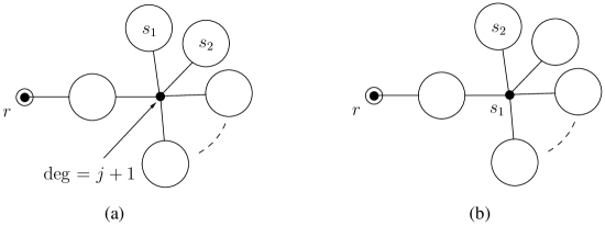
Figure 8: a) The case when $s_{1}\notin(r,s_{2})$. At least two balloons attached to the vertex of degree $j+1$ (excluding the rooted one) indicated in the figure have to have at least one vertex of degree $i+1$, namely $s_{1}$ and $s_{2}$. b) The case when $s_{1}\in(r,s_{2})$. At least one balloon attached to the vertex $s_{1}$ (excluding the rooted one) has to have at least one vertex of degree $i+1$ , namely $s_{2}$.

$$E_{N} = \sum_{i=0}^{N-1}\Bigg{(}\sum_{j=0}^{i-1}w_{j+1}[\zeta^{N}]\left\{\mathcal{Y}_{i}(\zeta)\sum_{n=2}^{j}\binom{j}{n}\underbrace{\left(\mathcal{L}_{i+1}(\zeta)-\mathcal{L}_{i}(\zeta)\right)^{n}}_{\text{$s_{1}$ and $s_{2}$ in here}}\mathcal{L}_{i}(\zeta)^{j-n}\right\}$$

$$\quad\quad\quad+~{}\underbrace{w_{i+1}}_{s_{1}}[\zeta^{N}]\left\{\mathcal{Y}_{i}(\zeta)\sum_{n=1}^{i}\binom{i}{n}\underbrace{\left(\mathcal{L}_{i+1}(\zeta)-\mathcal{L}_{i}(\zeta)\right)^{n}}_{\text{$s_{2}$ in here}}\mathcal{L}_{i}(\zeta)^{i-n}\right\}\Bigg{)}.$$

The outermost sum is over all possible maximal degrees. The first term in the brackets takes care of the case when $s_{1}\notin(r,s_{2})$. Then $j+1$ is the degree of the vertex where $(r,s_{1})$ and $(r,s_{2})$ start to differ. At least two of the subtrees attached to this vertex (excluding the rooted one) have to have at least one vertex of degree $i+1$, see Figure 8 (a). The second term in the brackets takes care of the case when $s_{1}\in(r,s_{2})$. At least one of the subtrees attached to $s_{1}$ (excluding the rooted one) has to have at least one vertex of degree $i+1$, see Figure 8 (b).

Lemma 4.9

For any $i$ and $N$ we have

$$[\zeta^{N}]\left\{\mathcal{L}_{i+1}(\zeta)-\mathcal{L}_{i}(\zeta)\right\}\leq\frac{w_{i+1}N}{i}[\zeta^{N}]\left\{\zeta\mathcal{L}_{i+1}(\zeta)^{i}\right\}.$$ (4.57)

• Use the Lagrange inversion theorem to obtain

  $$[\zeta^{N}]\left\{\mathcal{L}_{i+1}(\zeta)-\mathcal{L}_{i}(\zeta)\right\} = \frac{1}{N}[z^{N-1}]\left\{\ell_{i+1}(z)^{N}-\ell_{i}(z)^{N}\right\}$$ (4.58)

  $$= \frac{1}{N}[z^{N-1}]\left\{\left(\ell_{i+1}(z)-\ell_{i}(z)\right)\sum_{N_{1}+N_{2}=N-1}\ell_{i+1}(z)^{N_{1}}\ell_{i}(z)^{N_{2}}\right\}$$

  $$\leq w_{i+1}[z^{N-i-1}]\left\{\ell_{i+1}(z)^{N-1}\right\}$$

  Now use the Lagrange inversion theorem on the right hand side of (4.58) to obtain the result.

  $\square$

Lemma 4.10

For any $N$ we have

$$E_{N}\leq 2N^{2}\sum_{i=0}^{N-1}w_{i+1}^{2}[\zeta^{N-1}]\left\{\mathcal{Y}_{i+1}(\zeta)\mathcal{L}_{i+1}(\zeta)^{2i-1}\right\}.$$ (4.59)

• First note that

  $$\sum_{n=2}^{j}\binom{j}{n}\left(\mathcal{L}_{i+1}(\zeta)-\mathcal{L}_{i}(\zeta)\right)^{n}\mathcal{L}_{i}(\zeta)^{j-n}$$ (4.60)

  $$= \mathcal{L}_{i+1}(\zeta)^{j}-\mathcal{L}_{i}(\zeta)^{j}-j(\mathcal{L}_{i+1}(\zeta)-\mathcal{L}_{i}(\zeta))\mathcal{L}_{i}(\zeta)^{j-1}$$

  $$= (\mathcal{L}_{i+1}(\zeta)-\mathcal{L}_{i}(\zeta))\left(\sum_{j_{1}+j_{2}=j-1}\mathcal{L}_{i+1}(\zeta)^{j_{1}}\mathcal{L}_{i}(\zeta)^{j_{2}}-j\mathcal{L}_{i}(\zeta)^{j-1}\right)$$

  $$\leq j(\mathcal{L}_{i+1}(\zeta)-\mathcal{L}_{i}(\zeta))\left(\mathcal{L}_{i+1}(\zeta)^{j-1}-\mathcal{L}_{i}(\zeta)^{j-1}\right)$$

  $$= j(\mathcal{L}_{i+1}(\zeta)-\mathcal{L}_{i}(\zeta))^{2}\sum_{j_{1}+j_{2}=j-2}\mathcal{L}_{i+1}(\zeta)^{j_{1}}\mathcal{L}_{i}(\zeta)^{j_{2}}$$

  $$\leq j(j-1)(\mathcal{L}_{i+1}(\zeta)-\mathcal{L}_{i}(\zeta))^{2}\mathcal{L}_{i+1}(\zeta)^{j-2}.$$

  It is also clear that the above inequality holds inside $[\zeta^{N}]\left\{\cdot\right\}$ brackets. Therefore the sum over $j$ in (LABEL:errorterm) is estimated from above by

  $$\sum_{j=0}^{i-1}w_{j+1}[\zeta^{N}]\left\{\mathcal{Y}_{i}(\zeta)\sum_{n=2}^{j}\binom{j}{n}\left(\mathcal{L}_{i+1}(\zeta)-\mathcal{L}_{i}(\zeta)\right)^{n}\mathcal{L}_{i}(\zeta)^{j-n}\right\}$$ (4.61)

  $$\leq [\zeta^{N}]\left\{\mathcal{Y}_{i}(\zeta)(\mathcal{L}_{i+1}(\zeta)-\mathcal{L}_{i}(\zeta))^{2}\ell_{i}^{\prime\prime}(\mathcal{L}_{i+1}(\zeta))\right\}.$$

  Now use Lemma 4.9 to get

  $$[\zeta^{N}]\left\{\mathcal{Y}_{i}(\zeta)(\mathcal{L}_{i+1}(\zeta)-\mathcal{L}_{i}(\zeta))^{2}\ell_{i}^{\prime\prime}(\mathcal{L}_{i+1}(\zeta))\right\}$$ (4.62)

  $$= \sum_{N_{1}+N_{2}+N_{3}=N}[\zeta^{N_{1}}]\left\{\mathcal{Y}_{i}(\zeta)\ell_{i}^{\prime\prime}(\mathcal{L}_{i+1}(\zeta))\right\}[\zeta^{N_{2}}]\left\{\mathcal{L}_{i+1}(\zeta)-\mathcal{L}_{i}(\zeta)\right\}[\zeta^{N_{3}}]\left\{\mathcal{L}_{i+1}(\zeta)-\mathcal{L}_{i}(\zeta)\right\}$$

  $$\leq \frac{w_{i+1}^{2}}{i^{2}}N^{2}\sum_{N_{1}+N_{2}+N_{3}=N}[\zeta^{N_{1}}]\left\{\mathcal{Y}_{i}(\zeta)\ell_{i}^{\prime\prime}(\mathcal{L}_{i+1}(\zeta))\right\}[\zeta^{N_{2}}]\left\{\zeta\mathcal{L}_{i+1}(\zeta)^{i}\right\}[\zeta^{N_{3}}]\left\{\zeta\mathcal{L}_{i+1}(\zeta)^{i}\right\}$$

  $$= \frac{w_{i+1}^{2}}{i^{2}}N^{2}[\zeta^{N}]\left\{\zeta^{2}\mathcal{Y}_{i}(\zeta)\ell_{i}^{\prime\prime}(\mathcal{L}_{i+1}(\zeta))\mathcal{L}_{i+1}(\zeta)^{2i}\right\}.$$

  Next observe that

  $$\zeta\frac{\ell_{i}^{\prime\prime}(\mathcal{L}_{i+1}(\zeta))}{i^{2}}\mathcal{L}_{i+1}(\zeta)\leq\frac{\zeta\ell_{i+1}(\mathcal{L}_{i+1}(\zeta))}{\mathcal{L}_{i+1}(\zeta)}=1.$$ (4.63)

  Combining the above results we have the estimate

  $$\sum_{j=0}^{i-1}w_{j+1}[\zeta^{N}]\left\{\mathcal{Y}_{i}(\zeta)\sum_{n=2}^{j}\binom{j}{n}\left(\mathcal{L}_{i+1}(\zeta)-\mathcal{L}_{i}(\zeta)\right)^{n}\mathcal{L}_{i}(\zeta)^{j-n}\right\}$$ (4.64)

  $$\leq w_{i+1}^{2}N^{2}[\zeta^{N-1}]\left\{\mathcal{Y}_{i+1}(\zeta)\mathcal{L}_{i+1}(\zeta)^{2i-1}\right\}$$

  We get precisely the same estimate for the term in the second line in (LABEL:errorterm) (the calculations are even simpler) except that it is of order $N$ smaller and (4.59) follows.

  $\square$

The above lemma implies the following result.

Lemma 4.11

$$N^{\beta}\zeta_{0}^{N}E_{N}\longrightarrow 0\quad\quad\text{as}\quad\quad N\longrightarrow\infty.$$ (4.65)

• By Lemma 4.10

  $$N^{\beta}\zeta_{0}^{N}E_{N}\leq 2N^{\beta+2}\zeta_{0}^{N}\sum_{i=0}^{N-1}w_{i+1}^{2}[\zeta^{N-1}]\left\{\mathcal{Y}_{i+1}(\zeta)\mathcal{L}_{i+1}(\zeta)^{2i-1}\right\}.$$ (4.66)

  The sum on the right hand side has the same form as $Z_{1,N}$ with $\beta$ replaced by $2\beta$, cf. Equation (4.28). Equation (4.37), which describes the asymptotic behaviour of $Z_{1,N}$, can therefore be applied to show that the right hand side is $o(N^{2-\beta})$. Since $\beta>2$, this converges to zero as $N\longrightarrow\infty$.

  $\square$

Combining Lemmas 4.8 and 4.11 completes the proof of Theorem 4.1.

4.4 Generalization of $Z_{N}$

For technical reasons, which will be made clear in the next section, we need to generalize the sequence $Z_{N}$ as we now describe. If $r$ is the root of a tree we denote its unique nearest neighbour by $s$. Define

$$Z_{N}^{(R)}=\sum_{\tau\in\Gamma_{N}}w_{\sigma_{s}+R-1}\prod_{i\in V(\tau)\setminus\{r,s\}}w_{\sigma_{i}}.$$ (4.67)

In analogy with (3.4) and (3.5), define the generating functions

$$\mathcal{Z}(\zeta,R)=\sum_{N=1}^{\infty}Z_{N}^{(R)}\zeta^{N}$$ (4.68)

and

$$g_{R}(z)=\sum_{n=0}^{\infty}w_{n+R}z^{n}.$$ (4.69)

Clearly $Z_{N}=Z_{N}^{(1)},\mathcal{Z}(\zeta)=\mathcal{Z}(\zeta,1)$ and $g(z)=g_{1}(z)$. By the same arguments as for (3.6) we find the relation

$$\mathcal{Z}(\zeta,R)=\zeta g_{R}(\mathcal{Z}(\zeta)).$$ (4.70)

Let $\mathcal{Z}_{0,R}=\mathcal{Z}(\zeta_{0},R)$. The following Lemma is a generalization of Theorem 4.1.

Lemma 4.12

For the branching weights (4.1) which satisfy (4.2) it holds that

$$Z_{N}^{(R)}=\left(1-m+\frac{g_{R}^{\prime}(1)}{g(1)}\right)(1-m)^{-\beta}N^{-\beta}\zeta_{0}^{1-N}\left(1+o(1)\right).$$ (4.71)

• We write

  $$Z_{N}^{(R)}=Z_{1,N}^{(R)}+E_{N}^{(R)}$$ (4.72)

  in analogy with (4.5). One can show with the same methods as in the previous subsection that $\lim_{N\rightarrow\infty}E_{N}^{(R)}/Z_{N}=0$. Therefore we focus on the term $Z_{1,N}^{(R)}$, the contribution from trees with exactly one vertex of maximal degree. We split this term into two parts: one where the maximal degree vertex is the nearest neighbour of the root and another when it is not. We can then write

  $$Z_{1,N}^{(R)} = \sum_{i=0}^{N-1}w_{i+R}[\zeta^{N}]\left\{\zeta\mathcal{L}_{i}(\zeta)^{i}\right\}+\sum_{i=0}^{N-2}w_{i+1}[\zeta^{N}]\left\{\zeta\ell_{i,R}^{\prime}(\mathcal{L}_{i}(\zeta))\mathcal{Y}_{i}(\zeta)\mathcal{L}_{i}(\zeta)^{i}\right\}$$

  where we have defined

  $$\ell_{i,R}(z)=\sum_{n=0}^{i-1}w_{n+R}z^{n}.$$ (4.74)

  Let

  $$h(z)=\frac{z^{i+1}}{\ell_{i}(z)}$$ (4.75)

  and

  $$k(z)=\frac{\ell^{\prime}_{i,R}(z)z^{i+2}}{\ell_{i}(z)\left(\ell_{i}(z)-z\ell^{\prime}_{i}(z)\right)}.$$ (4.76)

  Using the Lagrange inversion formula for the functions $h$ and $k$ we find that

  $$[\zeta^{N}]\left\{\zeta\mathcal{L}_{i}(\zeta)^{i}\right\}=\frac{1}{N}[z^{N-i-1}]\left\{\left(\frac{i+1}{\ell_{i}(z)}-\frac{z\ell_{i}^{\prime}(z)}{\ell_{i}(z)^{2}}\right)\ell_{i}(z)^{N}\right\}$$ (4.77)

  and

  $$[\zeta^{N}]\left\{\zeta\ell_{i,R}^{\prime}(\mathcal{L}_{i}(\zeta))\mathcal{Y}_{i}(\zeta)\mathcal{L}_{i}(\zeta)^{i}\right\} = \frac{1}{N}[z^{N-i-2}]\Bigg{\{}\Bigg{(}\frac{(i+2)\ell_{i,R}^{\prime}(z)}{\ell_{i}(z)(\ell_{i}(z)-z\ell_{i}^{\prime}(z))}$$

  $$+~{}z\frac{d}{dz}\Bigg{(}\frac{\ell_{i,R}^{\prime}(z)}{\ell_{i}(z)(\ell_{i}(z)-z\ell_{i}^{\prime}(z))}\Bigg{)}\Bigg{)}\ell_{i}(z)^{N}\Bigg{\}}.$$

  We now use exactly the same arguments as in the proof of Lemma 4.8 to estimate the asymptotic behaviour of (LABEL:zr). One can show that the contribution from the second term in the curly brackets in (4.77) and (LABEL:zn2) is negligible. Then one can show that for any $\epsilon>0$

  $$\liminf_{N\rightarrow\infty}N^{\beta}\zeta_{0}^{N-1}Z_{1,N}^{(R)}\geq(1-\epsilon)\left(1-\left(m-\epsilon\right)\right)^{1-\beta}\left(1+\frac{g_{R}^{\prime}(1)}{g(1)-g^{\prime}(1)}\right)$$ (4.79)

  and

  $$\limsup_{N\rightarrow\infty}N^{\beta}\zeta_{0}^{N-1}Z_{1,N}^{(R)}\leq(1+\epsilon)\left(1-\left(m+\epsilon\right)\right)^{1-\beta}\left(1+\frac{g_{R}^{\prime}(1)}{g(1)-g^{\prime}(1)}\right).$$ (4.80)

  Since this holds for all $\epsilon>0$ the desired result follows.

  $\square$

5 The infinite volume limit

In this section we show that the measures $\nu_{N}$ converge as $N\longrightarrow\infty$ and we characterize the limits for the three different cases discussed in Section 3. If $m$ is the mean offspring probability defined in (3.10) then the three cases are: generic, critical case ($w_{1}<w_{c}$, $m=1$), the nongeneric, critical case ($w_{1}=w_{c}$, $m=1$) and the nongeneric, subcritical case ($w_{1}>w_{c}$, $m<1$).

All the results stated for generic trees have already been established [20] but are rederived here in a slightly different way. In the generic case, Equation (3.6) can be solved for $\mathcal{Z}(\zeta)$ close to the critical point $\zeta_{0}$ and one can then find the asymptotic behaviour of $Z_{N}$, the coefficients of $\mathcal{Z}(\zeta)$, see [28, Theorem 3.1]. In the non–generic critical case, the function $\mathcal{Z}(\zeta)$ has the same critical behaviour as in the generic case as long as $g^{\prime\prime}(1)<\infty$, see [25, Lemma A.2]. By the same arguments as in [22, 25] one finds the following result for $Z_{N}^{(R)}$.

Lemma 5.1

Under the stated assumption on the branching weights (3.1) and assuming that $m=1$ and $g^{\prime\prime}(\mathcal{Z}_{0})<\infty$ it holds that

$$Z_{N}^{(R)}=\sqrt{\frac{g(\mathcal{Z}_{0})}{2\pi g^{\prime\prime}(\mathcal{Z}_{0})}}\zeta_{0}g_{R}^{\prime}(\mathcal{Z}_{0})N^{-3/2}\zeta_{0}^{-N}\left(1+o(1)\right).$$ (5.1)

An analogous result for the asymptotic behaviour of $Z_{N}$, for a special choice of branching weights corresponding to nongeneric critical trees with $g^{\prime\prime}(1)=\infty$, is stated in [22, VI.18 and VI.19, page 407]. A generalization to $Z_{N}^{(R)}$ is straightforward and is stated in the following Lemma.

Lemma 5.2

For the nongeneric, critical branching weights defined by (4.1), with $2<\beta<3$ and $w_{1}=w_{c}$ we have

$$Z_{N}^{(R)}=C\zeta_{0}g_{R}^{\prime}(1)N^{-\frac{\beta}{\beta-1}}\zeta_{0}^{-N}\left(1+o(1)\right)$$ (5.2)

where $C>0$ is a constant.

We now prove that the measures $\nu_{N}$ converge as $N\rightarrow\infty$ provided that $Z^{(R)}_{N}$ has the right asymptotic behaviour. We call a self avoiding, infinite, linear path starting at the root a spine.

Theorem 5.3

If

$$Z^{(R)}_{N}=C\left(1-m+\zeta_{0}g_{R}^{\prime}(Z_{0})\right)N^{-\delta}\zeta_{0}^{-N}(1+o(1))$$ (5.3)

where $C$ is a positive constant and $\delta>1$, then the measures $\nu_{N}$ converge weakly, as $N\longrightarrow\infty$, to a probability measure $\nu$ which has the following properties:

• If $m=1$, $\nu$ is concentrated on the set of trees with exactly one spine having finite, independent, critical GW outgrowths defined by the offspring probabilities in (3.8). The numbers $i$ and $j$ of left and right outgrowths from a vertex on the spine are independently distributed by

  $$\phi(i,j)=\frac{1}{m}\zeta_{0}w_{i+j+2}Z_{0}^{i+j}.$$ (5.4)

• If $m<1$, $\nu$ is concentrated on the set of trees with exactly one vertex of infinite degree which we denote by $t$. The length $\ell$ of the path $(r,t)$ is distributed by

  $$\psi(\ell)=(1-m)m^{\ell-1}.$$ (5.5)

  The outgrowths from the path $(r,t)$ are finite, independent, subcritical GW trees defined by the offspring probabilities in (3.8). The numbers $i$ and $j$ of left and right outgrowths from a vertex $v\in(r,t),v\neq t$ are independently distributed by (5.4).

• First we prove existence of $\nu$. Since the metric space $(\Gamma,d)$ has the properties stated in Propositions (2.1 and 2.2) it is enough, as explained in [13, 17], to show that for any $k\in\mathbb{N}$ and $\tau^{\prime}\in\Gamma^{\prime}$ the probabilities

  $$\nu_{N}\left(\mathcal{B}_{\frac{1}{k}}\left(\tau^{\prime}\right)\right)$$ (5.6)

  converge as $N\longrightarrow\infty$. Since $\Gamma$ is compact, tightness is automatically fulfilled. The ball in (5.6) can be expressed as

  $$\mathcal{B}_{\frac{1}{k}}\left(\tau^{\prime}\right)=\left\{\tau\in\Gamma~{}|~{}L_{R}(\tau)=\tau_{0}\right\}$$ (5.7)

  where $R=k+1$ and $\tau_{0}=L_{R}(\tau^{\prime})$. Denote the number of vertices in $\tau_{0}$ of degree $R$ by $S$ and the number of vertices in $\tau_{0}$ at distance $R$ from the root by $T$. It is clear that $S+T\geq 0$.

  

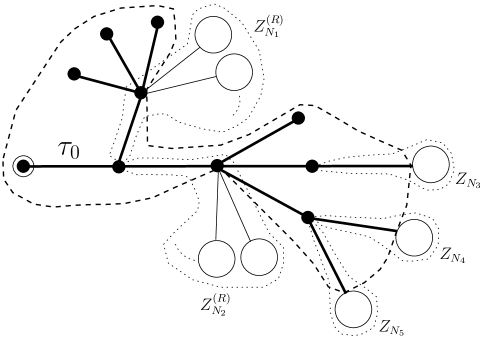
  Figure 9: An example of the set (5.7) where $R=4$, $S=2$ and $T=3$. When conditioning on trees of size $N$ one attaches the weights $Z^{(R)}_{N_{i}}$, $i=1\ldots S$ and $Z_{N_{j}}$, $j=S+1\ldots S+T$ as indicated in the figure.

  We can now write

  $$\nu_{N}\left(\left\{\tau\in\Gamma~{}|~{}L_{R}(\tau)=\tau_{0}\right\}\right)=$$

  $$\quad\quad\quad Z_{N}^{-1}W_{0}\sum_{N_{1}+\ldots+N_{S+T}=N-|\tau_{0}|+T+S}~{}\prod_{i=1}^{S}Z_{N_{i}}^{(R)}\prod_{j=S+1}^{S+T}Z_{N_{j}}$$ (5.8)

  where

  $$W_{0}=\prod_{\begin{subarray}{c}v\in V(\tau_{0})\setminus\{r\}\\ \sigma_{v},|(r,v)|\neq R\end{subarray}}w_{\sigma_{v}}$$ (5.9)

  is the weight of the tree $\tau_{0}$ (except the contribution from the vertices which are explicitly excluded), and $|(r,v)|$ denotes the length of the path $(r,v)$, see Fig. 9. For one of the indices $k$ in each term of the above sum it holds that $N_{k}\geq\frac{N-|\tau_{0}|+S+T}{S+T}$. Consider the contribution from terms for which $N_{n}>A$ for some other index $n\neq k$ and $A>0$. The indices $n$ and $k$ belong to one of the sets $\{1,\ldots,S\}$ and $\{S+1,\ldots,S+T\}$, a total of four possibilities. First assume that $S\geq 2$ and $n,k\in\{1,\ldots,S\}$. Using (5.3), this contribution can be estimated from above by

  $$C_{1}\zeta_{0}^{N}Z_{N}S^{2}\sum_{\begin{subarray}{c}N_{1}+\ldots+N_{S+T}=N-|\tau_{0}|+T+S\\ N_{1}\geq\frac{N-|\tau_{0}|+S+T}{S+T},~{}N_{2}>A\end{subarray}}Z_{N_{1}}^{(R)}\zeta_{0}^{N_{1}}~{}\prod_{i=2}^{S}Z_{N_{i}}^{(R)}\zeta_{0}^{N_{i}}\prod_{j=S+1}^{S+T}Z_{N_{j}}\zeta_{0}^{N_{j}}$$

  $$\leq C_{2}\left(\frac{(S+T)N}{N-|\tau_{0}|+T+S}\right)^{\delta}\sum_{\begin{subarray}{c}N_{3},\ldots,N_{S+T}\geq 1\\ N_{2}>A\end{subarray}}~{}\prod_{i=2}^{S}Z_{N_{i}}^{(R)}\zeta_{0}^{N_{i}}\prod_{j=S+1}^{S+T}Z_{N_{j}}\zeta_{0}^{N_{j}}$$

  $$\leq C_{3}\mathcal{Z}_{0,R}^{S-2}\mathcal{Z}_{0}^{T}\sum_{N_{2}>A}N_{2}^{-\delta}\leq C_{4}A^{1-\delta}$$ (5.10)

  where $C_{1}$, $C_{2}$, $C_{3}$ and $C_{4}$ are positive numbers independent of $N$ and $A$. Exactly the same upper bound is obtained, up to a multiplicative constant, for the other possible values of $k$ and $n$. The last expression goes to zero as $A\rightarrow\infty$ since $\delta>1$.

  The remaining contribution to the probability (5.8) is then

  $$\sum_{k=1}^{S+T}Z_{N}^{-1}W_{0}\sum_{\begin{subarray}{c}N_{1}+\ldots+N_{S+T}=N-|\tau_{0}|+T+S\\ N_{n}\leq A,~{}n\neq k\end{subarray}}~{}\prod_{i=1}^{S}Z_{N_{i}}^{(R)}\prod_{j=S+1}^{S+T}Z_{N_{j}}$$

  $$\xrightarrow[N\rightarrow\infty]{}W_{0}\zeta_{0}^{|\tau_{0}|-S-T}\Bigg{(}S(1-m+\zeta_{0}g_{R}^{\prime}(Z_{0}))\left(\sum_{n=1}^{A}Z_{n}^{(R)}\zeta_{0}^{n}\right)^{S-1}\left(\sum_{n=1}^{A}Z_{n}\zeta_{0}^{n}\right)^{T}$$

  $$\quad\quad\quad\quad\quad\quad\quad\quad\quad\quad\quad\quad+~{}T\left(\sum_{n=1}^{A}Z_{n}^{(R)}\zeta_{0}^{n}\right)^{S}\left(\sum_{n=1}^{A}Z_{n}\zeta_{0}^{n}\right)^{T-1}\Bigg{)}$$

  $$\xrightarrow[A\rightarrow\infty]{}W_{0}\zeta_{0}^{|\tau_{0}|-S-T}\left(S(1-m+\zeta_{0}g_{R}^{\prime}(Z_{0}))Z_{0,R}^{S-1}Z_{0}^{T}+TZ_{0,R}^{S}Z_{0}^{T-1}\right).$$ (5.11)

  This completes the proof of the existence of $\nu$. We now characterize $\nu$ separately for the cases $m=1$ and $m<1$.

  The case $m=1$: Let $\tau_{1}$ be a finite tree which has a vertex $s$ of degree one at a distance $R$ from the root. Let $A_{R}(\tau_{1})$ be the set of trees which have $\tau_{1}$ as a subtree and the property that if the subrees attached to $s$ which do not contain the root are removed one obtains $\tau_{1}$, see Fig. 10. It is clear that $A_{R}(\tau_{1})$ can be written as a finite union of pairwise disjoint balls as in $(\ref{ball})$. Therefore, by summing (5.11) over those balls we get

  $$\nu(A_{R}(\tau_{1}))=W_{1}\zeta_{0}^{|\tau_{1}|-1}$$ (5.12)

  where

  $$W_{1}=\prod_{v\in V(\tau_{1})\setminus\{r,s\}}w_{\sigma_{v}}.$$ (5.13)

  Note that Equation (5.12) has the same form as (5.11) with $S=0$ and $T=1$. Now define $A_{R}$ as the union of $A_{R}(\tau_{1})$ over all trees $\tau_{1}$ with the above properties. The sets $A(\tau_{1})$ and $A(\tau^{\prime}_{1})$ are disjoint if $\tau_{1}\neq\tau^{\prime}_{1}$ and therefore by summing (5.12) over $\tau_{1}$ we find that

  $$\nu(A_{R}) = \sum_{\tau_{1}}\Big{(}\prod_{v\in V(\tau_{1})\setminus\{r,s\}}w_{\sigma_{v}}\Big{)}\zeta_{0}^{|\tau_{1}|-1}=\Big{(}\zeta_{0}\sum_{i=0}^{\infty}(i+1)w_{i+2}Z_{0}^{i}\Big{)}^{R-1}$$ (5.14)

  $$= (\zeta_{0}g^{\prime}(Z_{0}))^{R-1}=m^{R-1}=1$$

  for all $R$. Therefore, by taking $R$ to infinity one finds that $\nu$ is concentrated on trees with exactly one spine with finite outgrowths. The distribution of the outgrowths follows from (5.12) and (5.13).

  

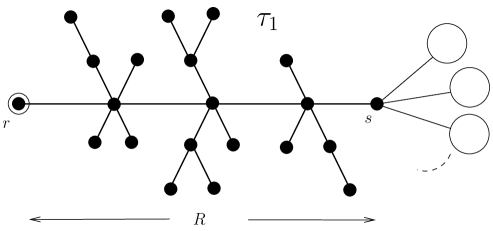
  Figure 10: An illustration of the set $A_{R}(\tau_{1})$.

The case $m<1$: Let $\tau_{2}$ be a finite tree which has a vertex $t$ of degree $R$ at a distance $\ell$ from the root. Let $A_{R,\ell}(\tau_{2})$ be the set of all trees which have $\tau_{2}$ as a subtree and the property that if the subtrees attached to $t$ in the $R$–th, $R+1$–st, $\ldots$ position clockwise from $(r,t)$ are removed one obtains $\tau_{2}$, see Fig. 11. Summing (5.11) as in the case $m=1$ one finds that

$$\nu(A_{R,\ell}(\tau_{2}))=W_{2}\zeta_{0}^{|\tau_{2}|-1}\left(1-m+\frac{g_{R}^{\prime}(1)}{g(1)}\right),$$ (5.15)

where

$$W_{2}=\prod_{v\in V(\tau_{2})\setminus\{r,t\}}w_{\sigma_{v}}.$$ (5.16)

Note that Equation (5.15) resembles (5.11) with $S=1$, $T=0$. Now define $A_{R,\ell}$ as the union of $A_{R,\ell}(\tau_{2})$ over all trees $\tau_{2}$ with the above properties. By summing (5.15) over $\tau_{2}$ we get

$$\nu(A_{R,\ell})=\left(1-m+\frac{g_{R}^{\prime}(1)}{g(1)}\right)m^{\ell-1}.$$ (5.17)

The sets $A_{R,\ell}$ are decreasing in $R$ so taking $R$ to infinity in (5.17) one finds, by the monotone convergence theorem, that the probability of exactly one vertex having an infinite degree and being at a distance $\ell$ from the root is $(1-m)m^{\ell-1}$. Summing this over $\ell$ gives 1 which shows that the measure is concentrated on trees with exactly one vertex of infinite degree. The distribution of the outgrowths follows from (5.15) and (5.16).

$\square$

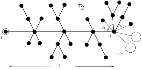
Figure 11: An illustration of the set $A_{R,\ell}(\tau_{2})$.

Theorem 5.4

Theorem 5.3 applies to the generic and nongeneric, critical ensembles in Lemmas 5.1 and 5.2 and the nongeneric, subcritical ensembles defined by (4.1) and (4.2).

• This follows from Lemmas 4.12, 5.1 and 5.2 since (5.3) holds with

  $$\delta=\left\{\begin{array}[]{ll}3/2&\quad\quad\text{generic, and nongeneric critical with $g^{\prime\prime}(1)<\infty$}\\ \beta/(\beta-1)&\quad\quad\text{nongeneric critical with $2<\beta<3$}\\ \beta&\quad\quad\text{nongeneric subcritical.}\end{array}\right.$$ (5.18)

  $\square$

The final result of this section concerns the size of the large vertex, in finite trees, which arises in the nongeneric, subcritical phase.

Theorem 5.5

Consider the nongeneric branching weights defined by (4.1) and (4.2). Let $C_{N,\epsilon}$ be the event that a tree in $\Gamma_{N}$ has exactly one vertex of maximal degree $\sigma_{\mathrm{max}}$ and $(1-m-\epsilon)N\leq\sigma_{\mathrm{max}}\leq(1-m+\epsilon)N$. For any $\epsilon,\delta>0$ there exists an $N_{0}\in\mathbb{N}$ such that

$$\nu_{N}\left(C_{N,\epsilon}\right)>1-\delta$$ (5.19)

for all $N\geq N_{0}$.

• This follows directly from the estimates (4.42), (4.44) and (4.47–4.53).

  $\square$

6 The spectral dimension of subcritical trees

In this section we will calculate the so called annealed spectral dimension of the nongeneric subcritical trees. A simple random walk on a graph $G$ is a sequence of nearest neighbour vertices, $\omega$, together with a probability weight

$$\prod_{t=0}^{|\omega|-1}\left(\sigma_{\omega_{t}}\right)^{-1}$$ (6.1)

where $\omega_{t}$ denotes the $(t+1)$-st vertex of $\omega$ and $|\omega|$ is the number of vertices in $\omega$. The random walk is a process where at time $t$ a walker, located at $\omega_{t}$, moves to one of its neighbours with probabilities $\left(\sigma_{\omega_{t}}\right)^{-1}$.

Let $p_{G}(t)$ be the probability that a simple random walk which begins at the root in $G$, is located at the root at time $t$. The spectral dimension of the graph $G$ is defined as $d_{s}$ provided that

$$p_{G}(t)\asymp t^{-d_{s}/2}$$ (6.2)

where we write $f(t)\asymp t^{-\gamma}$ if

$$\lim_{t\rightarrow\infty}\frac{\log{(f(t))}}{\log(t)}=-\gamma.$$ (6.3)

If $p_{G}(t)$ falls off faster than any power of $t$ then we say that $d_{s}=\infty$. The definition of $d_{s}$ is only useful on infinite graphs since on finite graphs, the return probability is asymptotically a positive constant. It is straightforward to verify that the spectral dimension of a connected, locally finite graph is independent of the choice of a root. The spectral dimension of the $d$–dimensional hyper–cubic lattice $\mathbb{Z}^{d}$ is $d_{s}=d$ in which case it agrees with our usual notion of dimension. For general graphs the spectral dimension need not be an integer and furthermore it might not exist.

For an infinite random graph $(\mathcal{G},\nu)$, where $\nu$ is a probability distribution on some set of graphs $\mathcal{G}$, one can define the spectral dimension in different ways. First of all the graphs can have, $\nu$ almost surely, a spectral dimension $d_{s}$ defined as above. Secondly, we define the annealed spectral dimension as $\bar{d}_{s}$ provided that

$$\langle p_{G}(t)\rangle_{\nu}\asymp t^{-\bar{d}_{s}/2}$$ (6.4)

where $\langle\cdot\rangle_{\nu}$ denotes expectation value with respect to $\nu$. These definitions need not agree and we will see an example where $\bar{d}_{s}$ exists and is finite, whereas $d_{s}$ is almost surely infinite. For a discussion of the spectral dimension of some random graph ensembles, see [19, 20, 26].

The Hausdorff dimension of a graph $G$ is defined in terms of how the volume of a graph ball $B_{R}(G)$ centered on the root scales with large $R$. The Hausdorff dimension is defined as $d_{H}$ if

$$|B_{R}(G)|\asymp R^{d_{H}}.$$ (6.5)

Similarly the annealed Hausdorff dimension is defined as $\bar{d}_{H}$ provided that

$$\langle|B_{R}(G)|\rangle_{\nu}\asymp R^{\bar{d}_{H}}.$$ (6.6)

The spectral and Hausdorff dimensions do not agree in general.

The Hausdorff dimension of subcritical trees is almost surely infinite and the annealed Hausdorff dimension is infinite. This follows from the fact that a vertex of infinite degree is almost surely at a finite distance from the root and that its expected distance from the root is finite. It is clear that the spectral dimension is almost surely infinite since a random walk will eventually hit the vertex of infinite degree and thereafter almost surely never return to the root. However, it turns out that the annealed spectral dimension is finite and takes the same values as in the case of subcritical caterpillars [27]. The main result of this section is the following theorem.

Theorem 6.1

For any $\beta>2$ the annealed spectral dimension of the subcritical trees defined by (4.1) and (4.2) is

$$\bar{d}_{s}=2(\beta-1)$$ (6.7)

provided it exists.

The return probabilities which we study to prove the above theorem, are most conveniently analysed through their generating functions. For a rooted tree $T$ define

$$Q_{T}(x)=\sum_{t=0}^{\infty}p_{T}(t)(1-x)^{t/2}.$$ (6.8)

The generating function variable $x$ is defined in this way for convenience in later calculations. Note that since $T$ is a tree only integer exponents appear on $1-x$. Let $p^{1}_{T}(t)$ be the probability that a random walk which leaves the root at time zero returns to the root for the first time after $t$ steps. Define the generating function

$$P_{T}(x)=\sum_{t=0}^{\infty}p^{1}_{T}(t)(1-x)^{t/2}.$$ (6.9)

By decomposing a walk which returns to the root into the first return walk, the second return walk etc. we find the relation

$$Q_{T}(x)=\sum_{n=0}^{\infty}(P_{T}(x))^{n}=\frac{1}{1-P_{T}(x)}.$$ (6.10)

Let $n$ be the smallest nonnegative integer for which $Q^{(n)}_{T}(x)$, the $n$–th derivative of $Q(x)$, diverges as $x\longrightarrow 0$. If

$$(-1)^{n}Q_{T}^{(n)}(x)\asymp x^{-\alpha}$$ (6.11)

for some $\alpha\in[0,1)$ then clearly

$$d_{s}=2(1-\alpha+n),$$ (6.12)

if $d_{s}$ exists. For random graphs, the same relation holds between the singular behaviour of $\langle Q^{(n)}_{T}\rangle_{\nu}$ as $x\longrightarrow 0$ and the annealed spectral dimension. We will prove Theorem 6.1 by establishing separately a lower bound and an upper bound on $\bar{d}_{s}$.

6.1 A lower bound on $\bar{d}_{s}$

We first present a formula for the $n$–th derivative of a composite function (see e.g. [4]) which will be used repeatedly.

Lemma 6.2

(Faà di Bruno’s formula) If $f$ and $g$ are $n$ times differentiable functions then

$$\frac{d^{n}}{dx^{n}}f(g(x))=\sum_{\sum_{i=1}^{n}iq_{i}=n}\frac{n!}{q_{1}!q_{2}!\cdots q_{n}!}f^{(q_{1}+\ldots+q_{n})}(g(x))\prod_{j=1}^{n}\left(\frac{g^{(j)}(x)}{j!}\right)^{q_{j}}.$$ (6.13)

The following lemma will be needed to obtain the lower bound on $\bar{d}_{s}$.

Lemma 6.3

Let $\mu$ be a subcritical GW measure on $\Gamma^{\prime}$ corresponding to the offspring probabilities (3.8). For any $n<\beta-1$ and any nonnegative integers $\theta_{1},\ldots,\theta_{k}$, $k\leq n$ such that $\theta_{k}\neq 0$ and $\sum_{a=1}^{k}a\theta_{a}\leq n$ it holds that

$$\left\langle\prod_{a=1}^{k}\left((-1)^{a}P^{(a)}_{T}(x)\right)^{\theta_{a}}\right\rangle_{\mu}<\infty$$ (6.14)

for all $x\in[0,1]$.

• The result is obvious for $x>0$ since the coefficients of $P_{T}(x)$ are smaller than one. First, take a fixed finite tree $T$ with root of degree one. Denote the degree of the nearest neighbour of the root by $N$ and the finite trees attached to that vertex by $T_{1},\ldots,T_{N-1}$. Then from [20] we have the recursion

  $$P_{T}(x)=\frac{1-x}{S_{T}(x)}$$ (6.15)

  where

  $$S_{T}(x)=N-\sum_{i=1}^{N-1}P_{T_{i}}(x).$$ (6.16)

  Note that $S_{T}(x)\geq 1$, since $P_{T_{i}}(x)\leq 1$ for all $i$. By Faà di Bruno’s formula (with $f(x)=1/x$, $g(x)=S_{T}(x)$) and throwing away negative powers of $S_{T}(x)$ we find that

  $$\frac{(-1)^{b}P_{T}^{(b)}(x)}{b!} \leq \sum_{\sum_{i=1}^{b}iq_{i}=b}\binom{q_{1}+\cdots+q_{b}}{q_{1},\ldots,q_{b}}\prod_{j=1}^{b}\left(\frac{(-1)^{j+1}S_{T}^{(j)}(x)}{j!}\right)^{q_{j}}$$

  $$+\sum_{\sum_{i=1}^{b-1}iq_{i}=b-1}\binom{q_{1}+\cdots+q_{b-1}}{q_{1},\ldots,q_{b-1}}\prod_{j=1}^{b-1}\left(\frac{(-1)^{j+1}S_{T}^{(j)}(x)}{j!}\right)^{q_{j}}$$

  where $\binom{q_{1}+\cdots+q_{b}}{q_{1},\ldots,q_{b}}$ is the multinomial coefficient. Looking at the product from the first sum we find that

  $$\prod_{j=1}^{b}\left(\frac{(-1)^{j+1}S_{T}^{(j)}(x)}{j!}\right)^{q_{j}}=\prod_{j=1}^{b}\sum_{p_{1}+\cdots+p_{N-1}=q_{j}}\binom{q_{j}}{p_{1},\ldots,p_{N-1}}\prod_{i=1}^{N-1}\left(\frac{(-1)^{j}P_{T_{i}}^{(j)}(x)}{j!}\right)^{p_{i}}.$$ (6.18)

  Expanding the above products and keeping track of the factors in each term which depend on the same outgrowth $T_{i}$, $i=1,\ldots,N-1$ we find that they are of the form

  $$C_{i}\prod_{j=1}^{b}\left(\frac{(-1)^{j}P_{T_{i}}^{(j)}(x)}{j!}\right)^{\alpha_{j}}$$ (6.19)

  where $\sum_{j=1}^{b}j\alpha_{j}\leq b$ and $C_{i}$ is a number independent of $T_{i}$ (the terms in the latter sum in (LABEL:fadibruno) are of the same form, if $b$ is replaced by $b-1$). The equality $\sum_{j=1}^{b}j\alpha_{j}=b$ holds only when $p_{i}=\alpha_{j}=q_{j}$ in which case $p_{a}=0$ if $a\neq i$ and $C_{i}=1$. The total contribution from such terms in (6.18) is therefore

  $$\sum_{i=1}^{N-1}\prod_{j=1}^{b}\left(\frac{(-1)^{j}P_{T_{i}}^{(j)}(x)}{j!}\right)^{q_{j}}.$$ (6.20)

  Now choose numbers $\theta_{1},\ldots,\theta_{k}$ such that $\theta_{k}\neq 0$ and $\sum_{a=1}^{k}a\theta_{a}\leq n$. Define $\Theta=\sum_{a=1}^{k}a\theta_{a}$. The following product of (LABEL:fadibruno) over $b$ has an upper bound

  $$\prod_{b=1}^{k}\left(\frac{(-1)^{b}P_{T}^{(b)}(x)}{b!}\right)^{\theta_{b}}\leq\sum_{i=1}^{N-1}\prod_{b=1}^{k}\left(\frac{(-1)^{j}P_{T_{i}}^{(b)}(x)}{b!}\right)^{\theta_{b}}$$

  $$~{}+C\sum_{M=1}^{\Theta}\sum_{\alpha(M)}\sum_{1\leq i_{1}<i_{2}<\cdots<i_{M}\leq N-1}\prod_{p=1}^{M}\prod_{b=1}^{k}\left(\frac{(-1)^{b}P_{T_{i_{p}}}^{(b)}(x)}{b!}\right)^{\alpha_{b,i_{p}}}+C$$

  where $\sum_{\alpha(M)}$ is a sum over nonnegative integers $\alpha_{b,i_{p}}$ which satisfy either

  $$\text{(i)}~{}\sum_{b=1}^{k}b\alpha_{b,i_{p}}<\Theta\quad\quad\text{or}\quad\quad\text{(ii)}~{}\sum_{b=1}^{k-1}b\alpha_{b,i_{p}}=\Theta$$ (6.21)

  and $C$ is a number which only depends on $k$ and $(\theta_{1},\ldots,\theta_{k})$. Taking the $\mu$ expectation value of the above inequality and using the fact that the subtrees $T_{i}$, $i=1,\ldots,N-1$ are identically and independently distributed and distributed as $T$ itself, yields

  $$\left\langle\prod_{b=1}^{k}\left(\frac{(-1)^{b}P_{T}^{(b)}(x)}{b!}\right)^{\theta_{b}}\right\rangle_{\mu}\leq$$

  $$\frac{C}{(1-m)g(1)}\sum_{M=1}^{\Theta}\sum_{\alpha(M)}\frac{g^{(M)}(1)}{M!}\prod_{p=1}^{M}\left\langle\prod_{b=1}^{k}\left(\frac{(-1)^{b}P_{T_{i_{p}}}^{(b)}(x)}{b!}\right)^{\alpha_{b,p}}\right\rangle_{\mu}+\frac{C}{1-m}.$$

  (6.22)

  Note, that $M\leq\Theta\leq n<\beta-1$ and thus $g^{(M)}(1)<\infty$. Therefore, for $x>0$, the right hand side of (6.22) is finite. To show that the left hand side is finite at $x=0$ we proceed by induction on the sequences $(\theta_{1},\theta_{2},\ldots,\theta_{k})$. We define a partial ordering on the set of such sequences in the following way (see also Fig. 12). Sequences $(\theta_{1},\ldots,\theta_{k})$ and $(\theta^{\prime}_{1},\ldots,\theta^{\prime}_{\ell})$ obey $(\theta^{\prime}_{1},\ldots,\theta^{\prime}_{\ell})<(\theta_{1},\ldots,\theta_{k})$ if and only if

  $$\text{(i)}~{}\sum_{i=1}^{\ell}i\theta^{\prime}_{i}<\sum_{i=1}^{k}i\theta_{i}\quad\quad\text{or}\quad\quad\text{(ii)}~{}\sum_{i=1}^{\ell}i\theta^{\prime}_{i}=\sum_{i=1}^{k}i\theta_{i}\quad\text{and}\quad\ell<k.$$

  For the smallest values, $k=1$ and $\Theta=1$, we find with the same calculations as above that

  $$\left\langle-P^{\prime}_{T}(x)\right\rangle_{\mu}\leq\frac{1}{1-m}.$$ (6.23)

  Next assume that (6.14) holds for for all sequences $(\theta^{\prime}_{1},\theta^{\prime}_{2},\ldots,\theta^{\prime}_{k^{\prime}})$ which are less than a given sequence $(\theta_{1},\theta_{2},\ldots,\theta_{k})$ with $k,\Theta\leq n$. Then, by (6.21), all the terms on the right hand side of (6.22) are finite and therefore the left hand side is finite for all $x\in[0,1]$. This shows that (6.14) holds for the sequence $(\theta_{1},\theta_{2},\ldots,\theta_{k})$.

  $\square$

Figure 12: A sequence $(\theta_{1},\theta_{2},\ldots,\theta_{k})$ is represented by a Young tableau where $\theta_{i}$ represents the number of rows of size $i$. The size of a tableau is $\Theta$ and the number of elements in the top row (grey boxes) is the value of $k$. The tableaux are first ordered by $\Theta$ and then by $k$ if possible. Tableaux with the same values of $\Theta$ and $k$ are incomparable.

Let $\nu$ be the measure corresponding to nongeneric subcritical trees as characterized in Theorem 5.3. To find a lower bound on $\bar{d}_{s}$ with respect to $\nu$ we study an upper bound on a suitable derivative of the $\nu$-average return probability generating function. Let $M_{\ell}$ be a linear graph of length $\ell$ with the root, $r$, at one end and a vertex of infinite degree, $t$, on the other end. Let $B_{\ell,k}$ be the set of trees with graph distance $\ell$ between $r$ and $t$ and such that at least one vertex on the path $(r,t)$ has degree $k$ and all the other vertices have degree no greater than $k$ (with the exception of $t$ of course). Define

$$\langle\cdot\rangle_{\nu,\tau\in A}=\nu(A)^{-1}\sum_{\tau\in A}\nu(\tau)\left(\cdot\right)$$ (6.24)

as the expectation value with respect to $\nu$ conditioned on the event $A$ and define

$$\phi(k)=\sum_{i+j=k-2}\phi(i,j).$$ (6.25)

We can write

$$\left\langle Q_{\tau}(x)\right\rangle_{\nu}=\sum_{\ell=1}^{\infty}\psi(\ell)\sum_{k=2}^{\infty}c(k,\ell)\langle Q_{\tau}(x)\rangle_{\nu,\tau\in B_{\ell,k}}$$ (6.26)

where

$$c(k,\ell)=\left(\sum_{i=2}^{k}\phi(i)\right)^{\ell-1}-\left(\sum_{i=2}^{k-1}\phi(i)\right)^{\ell-1}.$$ (6.27)

In a tree in $B_{\ell,k}$, denote the vertices on the path $(r,t)$ strictly between $r$ and $t$ by $s_{1},s_{2},\ldots,s_{\ell-1}$. Denote the outgrowths attached to $s_{i}$ by $T(s_{i})$, where $i=1,\ldots,\ell-1$ and denote the $j$-th outgrowth from $s_{i}$ by $T_{j}(s_{i})$ where $j=1,\ldots,\sigma_{s_{i}}-2$, see Fig. 13. The first return probability generating function for $T(s_{i})$ (viewing $s_{i}$ as the root) can be written in terms of the first return probability generating functions for $T_{j}(s_{i})$ in the following way

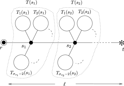
Figure 13: A tree from $B_{\ell,k}$.

$$P_{T(s_{i})}(x)=\frac{1}{\sigma_{s_{i}}-2}\sum_{j=1}^{\sigma_{s_{i}}-2}P_{T_{j}(s_{i})}(x).$$ (6.28)

Now take a $\tau\in B_{\ell,k}$. We can write

$$Q_{\tau}(x)=\sum_{\begin{subarray}{c}\omega:~{}r\rightarrow r\\ \text{on }M_{\ell}\end{subarray}}K_{\tau}(x,\omega)W_{\omega}(M_{\ell})(1-x)^{|\omega|/2}$$ (6.29)

where

$$K_{\tau}(x,\omega)=\prod_{\begin{subarray}{c}t=1\\ \omega_{t}\in\{s_{1},\ldots,s_{\ell-1}\}\end{subarray}}^{|\omega|-1}\frac{2}{2+(\sigma_{\omega_{t}}-2)(1-P_{T(\omega_{t})}(x))}$$ (6.30)

and

$$W_{\omega}(M_{\ell})=\prod_{t=0}^{|\omega|-1}(\sigma_{\omega_{t}}({M_{\ell}}))^{-1},$$ (6.31)

see [26]. Choose $n$ such that $n+1<\beta\leq n+2$. Differentiating $n$ times we get

$$\frac{(-1)^{n}Q^{(n)}_{\tau}(x)}{n!}=\sum_{n_{1}+n_{2}=n}\sum_{\begin{subarray}{c}\omega:~{}r\rightarrow r\\ \text{on }M_{\ell}\end{subarray}}W_{\omega}(M_{\ell})\frac{(-1)^{n_{1}}K^{(n_{1})}_{\tau}(x,\omega)}{n_{1}!}\frac{(-1)^{n_{2}}}{n_{2}!}\frac{d^{n_{2}}}{dx^{n_{2}}}(1-x)^{|\omega|/2}.$$ (6.32)

Let $\omega$ be a random walk and denote the maximal subsequence of $\omega$ which consists only of the vertices $s_{1},\ldots,s_{\ell-1}$ by $\omega^{\prime}$. Then

$$\frac{(-1)^{b}K^{(b)}_{\tau}(x,\omega)}{b!}=\sum_{n_{1}+\cdots+n_{|\omega^{\prime}|}=b}\prod_{t=1}^{|\omega^{\prime}|}\frac{(-1)^{n_{t}}}{n_{t}!}\frac{d^{n_{t}}}{dx^{n_{t}}}\left(\frac{2}{2+(\sigma_{\omega^{\prime}_{t}}-2)(1-P_{T(\omega^{\prime}_{t})}(x))}\right).$$

By Faà di Bruno’s formula we get

$$\frac{(-1)^{p}}{p!}\frac{d^{p}}{dx^{p}}\left(\frac{2}{2+(\sigma_{\omega^{\prime}_{t}}-2)(1-P_{T(\omega^{\prime}_{t})}(x))}\right)=$$

$$\frac{2}{2+(\sigma_{\omega^{\prime}_{t}}-2)(1-P_{T(\omega^{\prime}_{t})}(x))}\sum_{q_{1}+2q_{2}+\cdots+pq_{p}=p}\binom{q_{1}+\cdots+q_{p}}{q_{1},\ldots,q_{p}}$$

$$\times~{}\Big{(}\underbrace{\frac{2(\sigma_{\omega^{\prime}_{t}}-2)}{2+(\sigma_{\omega^{\prime}_{t}}-2)(1-P_{T(\omega^{\prime}_{t})}(x))}}_{(\ast)}\Big{)}^{q_{1}+\cdots+q_{p}}\prod_{a=1}^{p}\left(\frac{(-1)^{a}P^{(a)}_{T(\omega^{\prime}_{t})}(x)}{a!}\right)^{q_{a}}.$$

(6.33)

Now, $P_{T(\omega^{\prime}_{t})}(x)\leq 1-x$. Also note that the quantitiy ($\ast$) in (6.33) is increasing in $\sigma_{s_{i}}$ and since $\sigma_{s_{i}}\leq k$ for $i=1,\ldots,\ell-1$ we find that

$$(\ast)\leq\frac{2(k-2)}{2+(k-2)x}.$$ (6.34)

Observe that $\dfrac{2(k-2)}{2+(k-2)x}\leq 1$ for $k=2,~{}3$ and that $\dfrac{2(k-2)}{2+(k-2)x}\geq 1$ for $k\geq 4$. Finally, note that $\binom{q_{1}+\cdots+q_{p}}{q_{1},\ldots,q_{p}}\leq p^{p}$. Combining these results and using (6.28) we get the upper bound

$$\frac{(-1)^{b}K^{(b)}_{\tau}(x,\omega)}{b!}\leq b^{b}\left(\frac{2(k-2)}{2+(k-2)x}\right)^{(1-\delta_{k,2})(1-\delta_{k,3})b}$$

$$\sum_{n_{1}+\cdots+n_{|\omega^{\prime}|}=b}\prod_{t=1}^{|\omega^{\prime}|}\sum_{q_{1}+2q_{2}+\cdots+{n_{t}}q_{n_{t}}=n_{t}}\prod_{a=1}^{n_{t}}\frac{1}{(\sigma_{\omega^{\prime}_{t}}-2)^{q_{a}}}$$

$$\times~{}\sum_{p_{1}+\cdots+p_{\sigma_{\omega^{\prime}_{t}}-2}=q_{a}}\binom{q_{a}}{p_{1},\ldots,p_{\sigma_{\omega^{\prime}_{t}}-2}}\prod_{j=1}^{\sigma_{\omega^{\prime}_{t}}-2}\left(\frac{(-1)^{a}P^{(a)}_{T_{j}(\omega^{\prime}_{t})}(x)}{a!}\right)^{p_{j}}.$$

(6.35)

Expanding the above products and keeping track of the factors in each term which depend on the same outgrowth $T_{j}(s_{i})$, $i=1,\ldots,\ell-1$, $j=1,\ldots,\sigma_{s_{j}}-2$, we find that they are of the form

$$C_{ij}\prod_{a=1}^{n}\left((-1)^{a}P^{(a)}_{T_{j}(s_{i})}(x)\right)^{\theta_{a}}$$ (6.36)

where $\sum_{a=1}^{n}a\theta_{a}\leq n$ and $C_{ij}$ is independent of $T_{j}(s_{i})$. By Lemma 6.3, the expected value of (6.36) over the outgrowths $T_{j}(s_{i})$ is finite, and since the total number of terms on the right hand side of (6.35) is a polynomial in $|\omega^{\prime}|$ we find that

$$\left\langle(-1)^{b}K^{(b)}_{\tau}(x,\omega)\right\rangle_{\nu,\tau\in B_{\ell,k}}\leq H(|\omega|)\left(\frac{2(k-2)}{2+(k-2)x}\right)^{(1-\delta_{k,2})(1-\delta_{k,3})b}$$ (6.37)

where $H(|\omega|)$ is a polynomial with positive coefficients. From this inequality and the fact that $(-1)^{i}Q^{(i)}_{M_{\ell}}(0)$ is a polynomial in $\ell$ of degree $2i+1$, it follows that

$$\langle(-1)^{n}Q^{(n)}_{\tau}(x)\rangle_{\nu,\tau\in B_{\ell,k}}\leq\sum_{i=0}^{n}S_{i}(\ell)\left(\frac{2(k-2)}{2+(k-2)x}\right)^{(1-\delta_{k,2})(1-\delta_{k,3})i}$$ (6.38)

where $S_{i}(\ell)$, $i=0,\ldots,n$ are polynomials with positive coefficients. Noting that $c(k,\ell)\leq\phi(k)(\ell-1)$ we get from (6.26) that

$$\langle(-1)^{n}Q^{(n)}_{\tau}(x)\rangle_{\nu}\leq\sum_{i=0}^{n}\sum_{\ell=1}^{\infty}S_{i}(\ell)\psi(\ell)(\ell-1)\sum_{k=2}^{\infty}\phi(k)\left(\frac{2(k-2)}{2+(k-2)x}\right)^{(1-\delta_{k,2})(1-\delta_{k,3})i}.$$ (6.39)

The sum over $\ell$ is convergent since $\psi$ falls off exponentially and the sum over $k$ can be estimated by an integral yielding

$$\langle(-1)^{n}Q^{(n)}_{\tau}(x)\rangle_{\nu}\leq Cx^{\beta-n-2}\int_{x}^{\infty}\frac{y^{n+1-\beta}}{(2+y)^{n+1}}dy$$ (6.40)

where $C$ is a constant. If $\beta<n+2$ the last integral is convergent when $x\rightarrow 0$ but if $\beta=n+2$ it diverges logarithmically. In both cases we get the lower bound $\bar{d}_{s}\geq 2(1-\beta)$, provided $\bar{d}_{s}$ exists.

$\square$

6.2 An upper bound on $\bar{d}_{s}$

To find an upper bound on $\bar{d}_{s}$ we study a lower bound on a suitable derivative of the average return probability generating function. The aim is to cut off the branches of the finite outgrowths from the path $(r,t)$ so that only single leaves are left. We then use monotonicity results from [26] to compare return probability generating functions. As before we choose $n$ such that $n+1<\beta\leq n+2$. We begin by differentiating (6.26) $n$ times and throwing away every term in the sum over $\ell$ except the $\ell=2$ term

$$\left\langle(-1)^{n}Q^{(n)}_{\tau}(x)\right\rangle_{\nu}\geq(1-m)m\sum_{k=2}^{\infty}\phi(k)\left\langle(-1)^{n}Q^{(n)}_{\tau}(x)\right\rangle_{\nu,\tau\in B_{2,k}}.$$ (6.41)

Let $M_{2,k}$ be the graph constructed by attaching $k-2$ leaves to the vertex $s_{1}$ in $M_{2}$ defined in the previous section. Take a tree $\tau\in B_{2,k}$. Denote the nearest neighbours of $s_{1}$, excluding $r$ and $t$, by $u_{1},\ldots,u_{k-2}$. Denote the finite tree attached to $u_{i}$ by $U(u_{i})$, $i=1,\ldots,k-2$, and view $u_{i}$ as its root, see Fig. 14.

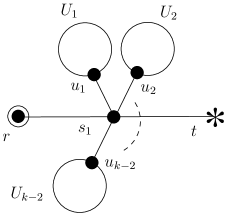
Figure 14: A graph $\tau\in B_{2,k}$.

We can write

$$Q_{\tau}(x)=\sum_{\begin{subarray}{c}\omega:~{}r\rightarrow r\\ \text{on }M_{2,k}\end{subarray}}F_{\tau}(x,\omega)W_{\omega}(M_{2,k})((1-x)^{|\omega|/2}$$ (6.42)

where

$$F_{\tau}(x,\omega)=\prod_{\begin{subarray}{c}t=1\\ \omega_{t}\in\{u_{1},\ldots,u_{k-2}\}\end{subarray}}^{|\omega|-1}\frac{1}{1+(\sigma_{\omega_{t}}-1)(1-P_{U(\omega_{t})}(x))}.$$ (6.43)

Define

$$H(x)=\sum_{\begin{subarray}{c}\omega:~{}r\rightarrow r\\ \text{on }M_{2,k}\end{subarray}}\ \left\langle F_{\tau}(x,\omega)\right\rangle_{\nu,\tau\in B_{2,k}}W_{\omega}(M_{\ell})\frac{d^{n-1}}{dx^{n}}(1-x)^{|\omega|/2}.$$ (6.44)

Differentiating once we easily find that

$$(-1)^{n}H^{\prime}(x)\leq\left\langle(-1)^{n}Q^{(n)}_{\tau}(x)\right\rangle_{\nu,\tau\in B_{2,k}}$$ (6.45)

and using the methods of [26, Section 4] we find that there exists a sequence $\xi_{i}$ converging to zero as $i\longrightarrow\infty$ on which

$$(-1)^{n}Q^{(n)}_{M_{2,k}}(\xi_{i})\leq(-1)^{n}H^{\prime}(\xi_{i}).$$ (6.46)

Using the relation (6.10) one can show that $(-1)^{n}Q_{\tau}(x)\geq(-1)^{n}P_{\tau}(x)$ for any $\tau$. Thus, we finally have

$$\left\langle(-1)^{n}Q^{(n)}_{\tau}(\xi_{i})\right\rangle_{\nu}\geq(1-m)m\sum_{k=2}^{\infty}\phi(k)(-1)^{n}P^{(n)}_{M_{2,k}}(\xi_{i})$$ (6.47)

on a sequence $\xi_{i}$ converging to zero. In [27] it is shown that

$$P^{(n)}_{M_{2,k}}(x)=(-1)^{n}\frac{n!(k-1)^{n-1}k}{(2+(k-2)x)^{n+1}}$$ (6.48)

and therefore the sum over $k$ in (6.47) can be estimated from the below by the same integral as in (6.40) up to a multiplicative constant. This proves that $\bar{d}_{s}\leq 2(\beta-1)$ provided $\bar{d}_{s}$ exists.

$\square$

7 Conclusions

We have studied an equilibrium statistical mechanical model of trees and shown that it has two phases, an elongated phase and a condensed phase. We have proven convergence of the Gibbs measures in both phases and on the critical line separating them. The main result is a rigorous proof of the emergence of a single vertex of infinite degree in the condensed phase. The phenomenon of condensation appears in more general models of graphs [1, 2] and it would be interesting to prove analogous results in those cases.

In the generic phase the annealed Hausdorff dimension is $\bar{d}_{H}=2$ and the annealed spectral dimension is $\bar{d_{s}}=4/3$, see [20]. The proof of this result relies only on the fact that the infinite volume measure is concentrated on the set of trees with exactly one spine having finite critical Galton–Watson outgrowths and that $g^{\prime\prime}(1)<\infty$. Therefore, it follows from Theorem 5.3 that $\bar{d}_{H}=2$ and $\bar{d}_{s}=4/3$ on the critical line when $g^{\prime\prime}(1)<\infty$.

It remains an open problem to calculate the dimension of trees on the critical line when $g^{\prime\prime}(1)=\infty$. It is easy to see that the annealed Hausdorff dimension is infinite in this case since the expected value of the degree of any vertex on the spine is infinite. However, we expect from the analogous case of caterpillars [27] and on the basis of scaling arguments [14, 16] that

$$d_{H}=\frac{\beta-1}{\beta-2}\quad\quad\quad\text{and}\quad\quad\quad d_{s}=\frac{2(\beta-1)}{2\beta-3}$$ (7.1)

holds almost surely, where $2<\beta\leq 3$. Note that by Theorem 5.3, the infinite volume measure is still concentrated on the set of trees with exactly one spine having critical Galton–Watson outgrowths. Therefore, a possible way to prove (7.1) is to follow the arguments in [20], but taking into account the different behaviour of critical Galton–Watson processes having $g^{\prime\prime}(1)=\infty$. Some results on such Galton–Watson processes can be found in [30].

In the condensed phase the Hausdorff and spectral dimension are almost surely infinite due to the infinite degree vertex. The same applies to the annealed Hausdorff dimension. However, the annealed spectral dimension takes the values $\bar{d}_{s}=2(\beta-1)$ where $\beta>2$. This is different from the value $\bar{d}_{s}=2$ which was obtained in [16] using scaling arguments. The reason is that the scaling ansatz used in [16] is apparently not valid when a vertex of infinite degree appears.
Acknowledgement. The work of SÖS was supported by the Eimskip fund at the University of Iceland. This work was partly supported by Marie Curie grant MRTN-CT-2004-005616 and the University of Iceland Research Fund. We are indebted to B. Durhuus, G. Miermont and W. Westra for helpful discussions.

References

- [1] M. E. Agishtein and A. A. Migdal, Critical behavior of dynamically triangulated quantum gravity in four dimensions, Nuclear Physics B, 385 (1992), pp. 395–412.
- [2] J. Ambjørn and J. Jurkiewicz, Four-dimensional simplicial quantum gravity, Physics Letters B, 278 (1992), pp. 42–50.
- [3] , Scaling in four-dimensional quantum gravity, Nuclear Physics B, 451 (1995), pp. 643–676.
- [4] G. E. Andrews, The theory of partitions, Cambridge Mathematical Library, Cambridge University Press, Cambridge, 1998. Reprint of the 1976 original.
- [5] G. Bennett, Probability inequalities for the sum of independent random variables, Journal of the American Statistical Association, 57 (1962), pp. 33–45.
- [6] P. Bialas, L. Bogacz, Z. Burda, and D. Johnston, Finite size scaling of the balls in boxes model, Nuclear Physics B, 575 (2000), pp. 599–612.
- [7] P. Bialas and Z. Burda, Phase transition in fluctuating branched geometry, Phys. Lett., B384 (1996), pp. 75–80.
- [8] , Collapse of 4d random geometries, Physics Letters B, 416 (1998), pp. 281–285.
- [9] P. Bialas, Z. Burda, and D. Johnston, Condensation in the backgammon model, Nucl. Phys., B493 (1997), pp. 505–516.
- [10] , Balls in boxes and quantum gravity, Nuclear Physics B - Proceedings Supplements, 63 (1998), pp. 763–765.
- [11] , Phase diagram of the mean field model of simplicial gravity, Nuclear Physics B, 542 (1999), pp. 413–424.
- [12] P. Bialas, Z. Burda, B. Petersson, and J. Tabaczek, Appearance of mother universe and singular vertices in random geometries, Nuclear Physics B, 495 (1997), pp. 463–476.
- [13] P. Billingsley, Convergence of probability measures, John Wiley & Sons Inc., New York, 1968.
- [14] Z. Burda, J. D. Correia, and A. Krzywicki, Statistical ensemble of scale-free random graphs, Phys. Rev., E64 (2001), p. 046118.
- [15] S. Catterall, G. Thorleifsson, J. Kogut, and R. Renken, Singular vertices and the triangulation space of the d-sphere, Nuclear Physics B, 468 (1996), pp. 263–276.
- [16] J. D. Correia and J. F. Wheater, The spectral dimension of non-generic branched polymer ensembles, Phys. Lett., B422 (1998), pp. 76–81.
- [17] B. Durhuus, Probabilistic Aspects of Infinite Trees and Surfaces, Acta Physica Polonica B, 34 (2003), p. 4795.
- [18] , Hausdorff and spectral dimension of infinite random graphs, Acta Physica Polonica B, 40 (2009), p. 3509.
- [19] B. Durhuus, T. Jonsson, and J. F. Wheater, Random walks on combs, J. Phys., A39 (2006), pp. 1009–1038.
- [20] , The spectral dimension of generic trees, Journal of Statistical Physics, 128 (2007), pp. 1237–1260.
- [21] M. R. Evans and T. Hanney, Nonequilibrium statistical mechanics of the zero-range process and related models, J. Phys. A, 38 (2005), pp. R195–R240.
- [22] P. Flajolet and R. Sedgewick, Analytic combinatorics, Cambridge University Press, Cambridge, 2009.
- [23] T. E. Harris, The theory of branching processes, Springer-Verlag, Berlin, 1963.
- [24] T. Hotta, T. Izubuchi, and J. Nishimura, Singular vertices in the strong coupling phase of four-dimensional simplicial gravity, Nuclear Physics B - Proceedings Supplements, 47 (1996), pp. 609–612.
- [25] S. Janson, Random cutting and records in deterministic and random trees, Random Struct. Algorithms, 29 (2006), pp. 139–179.
- [26] T. Jonsson and S. Ö. Stefánsson, The spectral dimension of random brushes, J. Phys. A: Math. Theor., 41 (2008), p. 045005.
- [27] , Appearance of vertices of infinite order in a model of random trees, J. Phys. A: Math. Theor., 42 (2009), p. 485006.
- [28] A. Meir and J. W. Moon, On the altitude of nodes in random trees, Canad. J. Math., 30 (1978), pp. 997–1015.
- [29] V. V. Petrov, Sums of independent random variables, Springer-Verlag, New York, 1975.
- [30] R. Slack, A branching process with mean one and possibly infinite variance, Z. Wahrsche, 9 (1968), pp. 139–145.
-
[31]
S. Ö. Stefánsson, Random brushes and non-generic trees,
Master’s thesis, University of Iceland, 2007.
Available at:
http://raunvis.hi.is/sigurdurorn/files/MSSOS.pdf. - [32] H. S. Wilf, Generatingfunctionology, A. K. Peters, Ltd., Natick, MA, USA, 2006.