Weak disorder: anomalous transport and diffusion are normal yet again

Abstract

We have carried out a detailed study of the motion of particles driven by a constant external force over a landscape consisting of a periodic potential corrugated by a small amount of spatial disorder. We observe anomalous behavior in the form of subdiffusion and superdiffusion and even subtransport over very long time scales. Recent studies of transport over slightly random landscapes have focused only on parameters leading to normal behavior, and while enhanced diffusion has been identified when the external force approaches the critical value associated with the transition from locked to running solutions, the regime of anomalous behavior had not been recognized. We provide a qualitative explanation for the origin of these anomalies.

Solid state surfaces frequently present periodic potentials marred by some disorder. Herein we show that an overdamped particle moving over such a potential in one dimension (1D) may exhibit anomalous behavior in the form of superdiffusion, subdiffusion, and even subtransport. Although we cannot prove that these are steady state regimes, our numerical simulation data show them to be present over time spans of several orders of magnitude.

That diffusion of particles over both periodic and random surfaces lead to some forms of anomalous behavior is of course well known and continues to attract a great deal of attention both theoretically and experimentally Theory ; anomalous ; PhysRevE70 ; SPIE ; katja2 ; Katja ; khoury:diffusion ; Lutz ; Grier ; Reimann . In periodic potentials with low friction, extremely long (in time) dispersionless transport regimes can be observed when forces exceed a critical force Katja . Moreover, in these same systems, in both overdamped and underdamped regimes, the diffusion coefficient versus the applied force presents a pronounced peak around the critical force that allows the coexistence of locked and running states Theory ; SPIE ; katja2 ; Katja ; khoury:diffusion . The The enhancement is quantitatively larger than the free particle diffusion coefficient. This behavior has been observed experimentally when tracking the motion of colloidal spheres through a periodic potential created with optical vortex traps Grier .

The enhancement of the diffusion coefficient is even more pronounced when disorder is also present Grier . This phenomenon has been tested by numerical simulations on a surface in which a small amount of spatial disorder in the form of a random potential is added to the periodic potential Reimann . Dramatic diffusive enhancement occurs even for very small amounts of disorder, e.g., when the amplitude of the random contribution of the potential is as small as $\sim 5\%$ of that of the periodic contribution.

Although dramatic, diffusive enhancement turns out to be only a limited aspect of the story because it is not the only manifestation of disorder. Here we present a range of additional anomalous transport and diffusion phenomena arising from weak disorder that have not been previously noted. Our model and the behaviors it exhibits are inspired by Grier ; Reimann .

We consider the overdamped motion of identical noninteracting Brownian particles moving in a 1D potential landscape $U(x)$ following the Langevin equation $\gamma\dot{x}(t)=-U^{\prime}(x)+F+\xi(t)$. Here $x$ is the position of the particle, $t$ denotes time, $\gamma$ is the dissipation parameter, $F$ is the applied force, and $\xi(t)$ is Gaussian thermal noise at temperature $T$. The correlation function of the noise obeys the fluctuation-dissipation relation $\langle\xi(t)\,\xi(t^{\prime})\rangle=2\gamma k_{B}T\delta(t-t^{\prime})$. The potential $U(x)$ consists of a periodic part, $V_{p}(x)=V_{0}\,\cos\left(2\pi x/\lambda_{p}\right)$, and a Gaussian spatially random contribution $V_{r}(x)$ with correlation function

$$g_{r}(x)\equiv\langle V_{r}(x)\,V_{r}(0)\rangle=\frac{V_{0}^{2}}{2}\exp\left(-\frac{2\pi^{2}x^{2}}{l_{r}^{2}}\right).$$ (1)

We need to choose parameters to capture the relative contribution of each, as well as their relative amplitudes and length scales. The relative contributions are determined by the parameter $\sigma$ in the combination

$$U(x)=(1-\sigma)V_{p}(x)+\sigma V_{r}(x),\qquad\sigma\in[0,1].$$ (2)

Furthermore, we have chosen the potential correlations $g_{r}(x)$ and $g_{p}(x)=(V_{0}^{2}/2)\cos\left(2\pi x/\lambda_{p}\right)$ to be equal at $x=0$, $g_{p}(0)=g_{r}(0)$. This ensures that the total potential amplitude is of order $V_{0}$ independently of $\sigma$. Also, with the particular choice $l_{r}=\lambda_{p}$ the two correlation functions are identical up to second order in a Taylor expansion.

The equation of motion can be rescaled into dimensionless form in terms of the spatial variable $z=2\pi x/\lambda_{p}$ and the temporal variable $\tau=[(2\pi)^{2}V_{0}/\gamma\lambda_{p}^{2}]t$. This yields

$$\dot{z}=(1-\sigma)f_{p}(z)+(\sigma/\lambda)f_{r}(z/\lambda)+{\mathcal{F}}+\eta(\tau),$$ (3)

where $f_{p}$ and $f_{r}$ are the dimensionless forces arising from $V_{p}$ and $V_{r}$, respectively, and $\eta$ is the dimensionless noise. The dimensionless parameters are

$$\lambda=\frac{l_{r}}{\lambda_{p}};\qquad{\mathcal{F}}=\frac{\lambda_{p}F}{2\pi V_{0}};\qquad{\mathcal{T}}=\frac{ḱk_{B}T}{V_{0}}.$$ (4)

Throughout this work we set ${\mathcal{T}}=0.01$ and $\lambda_{p}=2\pi$. Variations in ${\mathcal{T}}$ do not lead to any additional phenomenology. The specific choice of $\lambda_{p}$ is only important for passage between dimensionless and dimensioned units. An important note is that in these variables a decrease of $\lambda$ even for fixed $\sigma$ leads to an increase in the relative contribution of the random force.

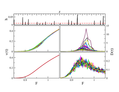
Figure 1: (Color online) Upper panel: Barriers $h$ of one realization of the total potential in a spatial domain of $\sim 32$ periods with $\lambda=0.5$ and ${\mathcal{F}}=1$. Middle and lower panels: Numerical data for 50 different disordered potentials and $N=100$ particles in each potential. Left panels: $v(\tau)$. Right panels: $D(\tau)$. Middle panels: $\lambda=1$. Lower panels: $\lambda=2\pi$ (regime of Ref. Reimann ). $\sigma=0.05$, $\tau=10^{4}$.

We have carried out numerical simulations of Eq. (3) over a large number (100) of particle trajectories and a large number of realizations of the random potential contribution (typically 50-100) in order to calculate the velocity and diffusion coefficient using the prescriptions

$$v(\tau)=\frac{\langle z(\tau)\rangle}{\tau},\qquad D(\tau)=\frac{\langle z^{2}(\tau)\rangle-\langle z(\tau)\rangle^{2}}{2\tau}.$$ (5)

The brackets $\langle\cdots\rangle$ denote averages over many trajectories and potentials. The numerical procedures are entirely standard. The usual assumption is that stationary values are reached at long times, an assumption that we show here to be at the very least questionable. Representative outcomes of this procedure are shown in the middle and lower panels of Fig. 1. These outcomes qualitatively capture an unanticipated range of behaviors in the right middle panel.

The velocity reaches a well-defined stationary value for any value of the force in the figure (left panels), even in the regime of sharp increase around ${\mathcal{F}}=1$. Also, as noted earlier, for the parameters used in Ref. Reimann , we see the enhancement of the (well defined) diffusion coefficient around the critical deterministic force ${{\mathcal{F}}}_{c}$, as discussed in that work (lower right panel). However, entirely different behavior is now seen in the middle right panel of the figure, which shows huge variations in the diffusion coefficient. Note that these variations extend over orders of magnitude. The question then is - what leads to these variations and why were they not identified in Ref. Reimann ?

The answer lies in the choice of the correlation length of the random potential. In Reimann the correlation length is much greater than a single period of the periodic potential, that is, the randomness is very smooth. However, entirely different behavior is seen when the random potential is more corrugated, as it is in our case. We see that the traditional diffusion coefficient is no longer well-defined in this regime but instead presents very strong fluctuations around its peak value, making a precise estimation of $D$ questionable. Note also the very large scale differences of the middle and lower right panels of the figure. These are signatures of anomalous behavior. While it is not clear whether a well-defined value of $D$ would be obtained at much longer times beyond our computational reach, we have repeated these calculations for many more particles and potential realizations and continue to find this variability.

To understand the origin of these anomalies, in the upper panel of Fig. 1 we plot the barriers $h$ of the total potential $U(z)-{\mathcal{F}}z$ for a particular realization of the random potential. The heights and locations of the barriers are random, and most of them exceed the thermal energy (dashed line). Smaller values of $\lambda$ lead to a greater number and height of the barriers. As a particle moves along such a landscape, it must overcome these barriers, some of which are extremely high. Indeed, $V_{r}(z)$ allows for barriers of any height, limited only by finite system sizes and simulation times. Thus, even with a small amount of disorder the particle motion is dominated by random waiting times due to the dispersion of the barrier heights, and a few long waiting times that greatly influence the outcome. We go on to show that the diffusion anomaly in Fig. 1 is a consequence of such landscapes and that it is qualitatively different from a simple large enhancement of the diffusion coefficient. In fact, strong fluctuations in the usual ensemble calculation of the diffusion coefficient point to the fact that our system is exhibiting behavior reminiscent of aging or of weak ergodicity breaking Sokolov ; Bouchaud ; Klages over the time scales of our simulations. We approach the problem with this observation in mind.

Our numerical results are collected as follows. Particles are initially located at random positions uniformly extended over a region of about 1000 sites, and for each we observe the times $t_{p}$ that it takes a single particle to cover the underlying spatial period $\lambda_{p}$ over the course of its trajectory over a long time. We collect these statistics for many particles and many realizations of the random potential. If the motion of the particles is “normal” then following the reasoning in Theory ; Lutz and also used in Reimann leads to the average velocity and diffusion coefficient expressions

$$v=\frac{\lambda_{p}}{\langle t_{p}\rangle},\qquad D=\frac{\lambda_{p}^{2}}{2}\,\frac{\langle\Delta^{2}t_{p}\rangle}{\langle t_{p}\rangle^{3}}.$$ (6)

Here $\langle t_{p}\rangle$ is the average of the $t_{p}$ over all trajectories, particles, and potential realizations and $\langle\Delta^{2}t_{p}\rangle$ is their dispersion about the average. It is of course evident that these expressions are only well defined if the first and second moments of the distribution of the $t_{p}$ are finite. We present numerical evidence that indicates that in the presence of a small amount of disorder in the potential the distribution $P(t_{p})$ of the time $t_{p}$ to cover a single period can have a power-law tail for long stretches of time,

$$P(t_{p})\sim t_{p}^{-\beta}.$$ (7)

This behavior leads to the observed anomalies if $\beta$ is sufficiently small. For $\beta>3$, the first and second moments are finite, so transport and diffusion are normal. In the range $2<\beta<3$, the first moment is finite but the second moment diverges. This leads to a finite average velocity $v$, but the diffusion coefficient as defined in Eq. (6) diverges (superdiffusion). In the interval $3/2<\beta<2$ the first moment diverges and the average velocity thus vanishes (subtransport). The second moment again diverges (superdiffusion). For $1<\beta<3/2$ we again have substransport, and the diffusion coefficient decays to zero (subdiffusion). In this case the particle remains extremely localized around its point of origin. Interestingly, we observe all of these behaviors.

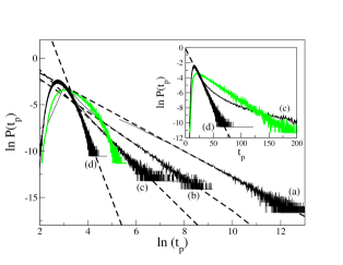
Figure 2: (Color online) Log-log plot of the time distribution for different values of $\lambda$. (a) $\lambda=0.1$ ($\beta=1.4$), (b) $\lambda=0.4$ ($\beta=1.8$), (c) $\lambda=0.8$ ($\beta=2.6$), and (d) $\lambda=2\pi$ ($\beta=6.9$). The parameter values are ${\mathcal{F}}=1$ and $\sigma=0.05$. Inset: Log plot of $P(t_{p})$ for cases (c) and (d). Also shown is the exponential distribution for a purely periodic potential with the same force (green online).Time $\tau\geq 10^{4}$ as needed to obtain reliable histograms.

To obtain values of $\beta$, we focus on the tails of the distribution. If they follow a power law, exponents $\beta$ are estimated, as depicted in Fig. 2. In the upper panel of Table 1, we present a set of typical results of simulations leading to different values of the exponent $\beta$, obtained for two levels of disorder and for different forces. We observe that, in many cases, a value $\beta<3$ associated with anomalous behavior is found. Table 1 also shows that a lower level of disorder ($\sim 2\%$) leads to higher exponents. These estimated values are of course informative but should not be interpreted too narrowly because they are based on sparse statistics. For the sake of comparison with Ref. Reimann , we also show the case $\lambda=2\pi$ for a $5\%$ level of disorder. We observe what we expected from Eq. (3) when $\lambda$ increases, that is, the effect of the random part of the potential is greatly muted. This implies that most of the exponents are in the range $\beta>3$ (normal behavior) for the range of forces selected, which explains why the anomalies explored herein were not found in Ref. Reimann . Much smaller forces would need to be explored to find robust anomalous behavior there. For our parameter choices, using $\lambda$ as a control parameter (keeping $\mathcal{F}$ fixed) also leads to $\beta$ values covering all the possible regimes (see bottom panel of Table 1).

	0.82	0.92	0.95	0.98	1.0	1.02	1.05
0.05 ($\lambda=1$)	1.1	1.7	2.2	2.7	2.9	3.6	4.8
0.02 ($\lambda=1$)	1.4	2.3	3.2	4.3	4.6	$>5$	$>5$
0.05 ($\lambda=2\pi$)	2.2	3.0	$>5$	$>5$	$>5$	$>5$	$>5$
	0.1	0.4	0.6	0.8	1.2	1.4	$2\pi$
0.05 (${\mathcal{F}}=1$)	1.4	1.8	2.1	2.6	3.5	4.0	$>5$

Table 1: Upper panel: Exponents $\beta$ for different values of the force and two values of $\sigma$ and $\lambda$. Bottom panel: Exponents $\beta$ for different values of $\lambda$, with ${\mathcal{F}}=1$ and $\sigma=0.05$

As the value of $\beta$ increases with increasing $\lambda$, the shape of the distribution $P(t_{p})$, particularly its tail, changes from a power law form to the more typical exponential associated with normal behavior. This occurs because changing $\lambda$ induces a change of the effective contribution of the random part of the potential, as already noted earlier. We pointed out that increasing $\lambda$ diminishes the effects of the disorder. In fact, case (d) of Fig. 2 is no longer a power law, as shown in the inset of the figure, but is instead better described as an exponential, characteristic of normal diffusive behavior.

Figure 3: (Color online) Log-log plot of the time evolution of the velocity (left) and of the diffusion coefficient (right) for different values of $\lambda$: $\lambda=0.1$ (solid line), $\lambda=0.4$ (dashed line), $\lambda=0.8$ (dotted line) and $\lambda=2\pi$ (dotted-dashed line). Parameter values: $\sigma=0.05$, ${\mathcal{F}}=1$. Number of potential realizations: 100, except for $\lambda=2\pi$ where 20 realizations are sufficient.

Finally, temporal evolutions of the velocity and the diffusion coefficient for the four different regimes of behavior are shown in Fig. 3. They are in qualitative agreement with this analysis, at least during a transient of several decades. The subtransport regimes of the two cases with the lowest values of $\lambda$ are clearly seen, as are the subdiffusive and superdiffusive behaviors of the diffusion coefficient.

In conclusion, we have carried out a detailed numerical study of the motion of particles driven by a constant external force over a one-dimensional landscape consisting of a periodic potential modified by a small amount of spatial disorder. We have identified a set of dramatic anomalous behaviors as diverse as subtransport, subdiffusion, and superdiffusion on the same surfaces as the driving force or the random corrugation length is varied. These behaviors are observed over very long time scales. Their asymptotic persistence behavior is not known. Earlier studies have focused only on parameters of normal behavior Grier ; Reimann , and while they have identified the occurrence of enhanced diffusion when the external force approaches the critical value associated with the transition from locked to running solutions, they have not recognized the regime of anomalous behavior.

The regimes that exhibit these anomalous behaviors are identified by the correlation length $l_{r}$ of the random portion of the potential. We find anomalous behavior when $l_{r}\lesssim\lambda_{p}$, the period of the periodic portion, that is, when the periodic potential is slightly corrugated over short distances. Earlier studies had focused on the regime $l_{r}=2\pi\lambda_{p}$, that is, on regimes of very long smooth variation of the random contribution to the potential. Experiments with more corrugated surfaces than have been used so far Grier are clearly desirable to see the effects that we have identified.

It would of course also be desirable to extend these studies to higher dimensions and to find an analytic characterization of these systems, one which would allow insight into the asymptotic behavior. Such an analysis has recently been presented for the case of a piecewise linear random potential Denisov , but seems not yet to be available for the more realistic potentials considered here.

This work was supported by the MICINN (Spain) under the project FIS2009-13360 (AML, MK and JMS), by Generalitat de Catalunya Projects 2009SGR14 (JMS, MK) and 2009SGR878 (AML), and the grant FPU-AP2005-4765 (MK). KL gratefully acknowledges the NSF under Grant No. PHY-0855471.

References

- (1) P. Reimann, C. Van den Broeck, H. Linke, P. Hänggi, J.M. Rubi, and A. Pérez-Madrid, Phys. Rev. Lett 87, 010602 (2001).
- (2) J.M. Sancho, A.M. Lacasta, Katja Lindenberg, I.M. Sokolov and A.H. Romero, Phys. Rev. Lett. 92, 250601 (2004).
- (3) A. M. Lacasta, J.M. Sancho, A.H. Romero, I.M. Sokolov, and Katja Lindenberg, Phys. Rev. E 70, 051104 (2004).
- (4) Katja Lindenberg, A.M. Lacasta, J.M. Sancho, and A.H. Romero, Proc. SPIE 5845, 201 (2005).
- (5) Katja Lindenberg, A.M. Lacasta, J.M. Sancho and A.H. Romero, New Journal of Physics 7, 29 (2005).
- (6) Katja Lindenberg, J.M. Sancho, A.M. Lacasta and I.M. Sokolov, Phys. Rev. Lett. 98, 020602 (2007).
- (7) M. Khoury, James P. Gleeson, J. M. Sancho, A.M. Lacasta, and Katja Lindenberg, Phys. Rev. E 80, 021123 (2009).
- (8) B. Lindner, M. Kostur, and L. Schimansky-Geier, Fluct. Noise Lett. 1, R25 (2001).
- (9) Sang-Hyuk Lee, and David G. Grier, Phys. Rev. Lett 96, 190601 (2006).
- (10) P. Reimann and R. Eichhorn, Phys. Rev. Lett. 101, 180601 (2008).
- (11) Y. He. S. Burov, R. Metzler, and E. Barkai, Phys. Rev. Lett. 101, 058101 (2008); I.M. Sokolov, E. Heinsalu, P. Hänggi, and I. Goychuck, Europhys. Lett. 86, 30009 (2009).
- (12) J. P. Bouchaud, J. De Physique 12, 1705 (1992).
- (13) E. Barkai, “Anomalous Kinetics Leads to Weak Ergodicity Breaking,” in Anomalous Transport, edited by R. Klages, G. Radons, and I. M. Sokolov (Wiley-VCH, Weinheim, 2008).
- (14) S.I. Denisov, E.S. Denisova, and H. Kantz, Europhys. J. B76, 1 (2010).