Fourier transformation and response functions

Abstract

We improve on Fourier transforms (FT) between imaginary time $\tau$ and imaginary frequency $\omega_{n}$ used in certain quantum cluster approaches using the Hirsch-Fye method. The asymptotic behavior of the electron Green’s function can be improved by using a “sumrule” boundary condition for a spline. For response functions a two-dimensional FT of a singular function is required. We show how this can be done efficiently by splitting off a one-dimensional part containing the singularity and by performing a semi-analytical FT for the remaining more innocent two-dimensional part.

Quantum cluster cluster theories, such as the dynamical cluster approximation (DCA) or the cellular dynamical mean-field theory (CDMFT),Jarrell make it possible to calculate dynamical quantities, e.g., electron Green’s functions or response functions, for strongly correlated systems. These calculations, however, are numerically very demanding. In the Hirsch-FyeHirsch method for solving the resulting cluster problem, one has to switch between imaginary times $\tau$ and imaginary frequencies $\omega_{n}$, which requires Fourier transforms (FT). In this paper we address efficient methods for performing FT in this context. In the weak-coupling versionRubtsov ; CT ; Assaad of continuous time approachesRubtsov ; CT ; Assaad ; CTAUX properties can be very easily measured directly in frequency space and no FT is needed.

The FT of the electron Green’s function has to be performed with great care, and it is important to obtain the correct asymptotic behavior for large $\omega_{n}$.Blumer ; Comanac ; Knecht ; Gull Inaccuracies for large $\omega_{n}$ can lead to problems, for instance in the DMFT description of a Mott transition.Blumer The large $\omega_{n}$ behavior can be greatly improved if exact moments are calculated. The FT can then be performed using a natural spline, which works well for a symmetric half-filled Hubbard model.Blumer For a nonsymmetric or doped Hubbard model, however, the accuracy is not optimum. Here we show how this can be improved by introducing “sumrule” boundary conditions for the spline interpolation.

The main part of this paper deals with response functions. This is important not only for studying susceptibilities but also for diagrammatic extensions of the dynamical mean-field theory, such as the dynamical vertex approximationdynamical and the dual fermion method.dual The most convenient way of of calculating them within DCA is to work directly in $\omega_{n}$-space. Yet, in the Hirsch-Fye method this requires FT for functions $g(\tau_{i},\tau_{j})$ depending on two imaginary times, $\tau_{i}$ and $\tau_{j}$, for each Monte-Carlo step. The FT is complicated by the fact that these functions have singularities and that the precise asymptotic behavior is difficult to work out. We show that a very efficient solution is to split up $g(\tau_{i},\tau_{j})$ into two parts. One part, $g^{(0)}(\tau_{i}-\tau_{j})$, depends only on the difference $\tau_{i}-\tau_{j}$ and contains the singularity. The second part, $\delta g(\tau_{i},\tau_{j})$ depends on both variables independently but is well behaved. To perform spline interpolations in both variables is very time consuming. We show how the FT can be performed in a very efficient way for $\delta g(\tau_{i},\tau_{j})$.

If $G(\tau)$ is only known for discrete values of $\tau$ separated by $\Delta\tau$, a direct FT can only give accurate results up to $\omega_{n}\sim 1/\Delta\tau$. To improve the accuracy for large $\omega_{n}$, on can subtract a model Green’s function, $G_{m}(\tau)$, from $G(\tau)$, where $G_{m}$ has the right asymptotic behavior. The difference, $G(\tau)-G_{m}(\tau)$, is then FT and $G_{m}(i\omega_{n})$ is added. For instance, $G_{m}(\tau)$ can be obtained from perturbation theory.Freericks Alternatively, one can calculate the lowest moments of the spectral function exactly from appropriate expectation values.Blumer $G_{m}(i\omega_{n})$ can be chosen so that these moments are exactly satisfied, meaning that the corresponding coefficients in a $(1/\omega_{n})$ expansion of $G_{m}(i\omega_{n})$ are correct. $G(\tau)-G_{m}(\tau)$ is then FT using a natural spline.Blumer If the FT of $G(\tau)-G_{m}(\tau)$ correctly gives the lowest moments equal to zero, it follows that the corresponding moments of $G(i\omega_{n})$ are correct.

To illustrate this, we consider the relation between the spectral function, $A(\omega)$, and $G(\tau)$

$$G(\tau)=\int_{-\infty}^{\infty}{e^{-\omega\tau}\over 1+e^{-\omega\beta}}A(\omega)d\omega,$$ (1)

where $\beta=1/T$ and $T$ is the temperature. This gives the following, very useful, relations

$$G^{(n)}(0)+G^{(n)}(\beta)=\int_{-\infty}^{\infty}(-\omega)^{n}A(\omega)d\omega\equiv(-1)^{n}M_{n},$$ (2)

where $G^{(n)}(\tau)=d^{n}G(\tau)/d\tau^{n}$ and $M_{n}$ is the $n$th moment. For large $\omega_{n}$, $G(\omega_{n})\sim\sum_{k}M_{k}/(i\omega_{n})^{k+1}$. For the difference $\Delta G(\tau)\equiv G(\tau)-G_{m}(\tau)$, it then follows that

$$\Delta G^{(n)}(0)+\Delta G^{(n)}(\beta)=0\hskip 28.45274ptn=0,1,2,$$ (3)

if $G_{m}$ has the correct 0th, 1st and 2nd moments.

Let $\Delta G(\tau)$ be given for $n$ $\tau$-values, $\tau_{1}$, …, $\tau_{n}$. In a third order spline, each interval between two $\tau$-values is interpolated with a third order polynomial. It is required that the polynomials give the correct $\Delta G(\tau_{i})$ and that the first two derivatives are continuous at each $\tau_{i}$. There are then $4(n-1)$ unknown coefficients and $4(n-2)+2$ conditions. We then have to provide two more conditions.

For a natural spline, it is assumed that $\Delta G^{(2)}(0)=\Delta G^{(2)}(\beta)=0$, while the first derivatives are left open. The assumption about $\Delta G^{(2)}$ is too strong, since we only know that $\Delta G^{(2)}(0)+\Delta G^{(2)}(\beta)=0$. The second moment is nevertheless correct, since it only depends on the sum. The incorrect assumption about $\Delta G^{(2)}$, however, influences the estimates of $\Delta G^{(1)}$ and $\Delta G^{(1)}(0)+\Delta G^{(1)}(\beta)=0$ is in general not satisfied. This leads to incorrect results already for the important first moment. Due to symmetry, the natural spline may give $\Delta G^{(1)}(0)+\Delta G^{(1)}(\beta)=0$ in special cases, e.g., at half-filling for the symmetric Hubbard model.

A better approach is to use the two conditions of Eq. (3) for $n=1$ and 2. We refer to this as the sumrule spline. This gives correct first and second moments and large $\omega_{n}$ behavior, even if the estimates of $\Delta G^{(n)}(0)$ and $\Delta G^{(n)}(\beta)$ individually are not accurate.

Fig.1 compares the two approaches for the two-dimensional (2d) Hubbard model in the DCA. We have used $t=-0.4$ and $t_{p}=-0.3t$ for the nearest and next nearest neighbor hopping, respectively, $U=8|t|$ for the on-site Coulomb interaction and $\beta|t|=12$. All energies are in eV. The occupancy is $n=0.9$ and we considered an eight site cluster. The number of $\tau$-points is $N_{\tau}=120$. For large $\omega_{n}$, the local Green’s function behaves as $G(z)\sim 1/(z-a-b/z)$, where $z=i\omega_{n}$ and $a=M_{1}$ and $b=M_{2}-M_{1}^{2}$ are given by the first two moments. If we define $\Sigma(z)=z-G^{-1}(z)$, we have

$$\Sigma(z)\sim a+b/z$$ (4)

for large $|z|$. The figure shows that Re $\Sigma(z)\to a$ is obtained for the sumrule spline but not for the natural spline. Also for Im $\Sigma(z)\sim b/z$ (not shown in the figure) the natural spline is less accurate than the sumrule spline, since an error in $M_{1}$ also enters in $b$, but for large $|z|$ the error for Im $\Sigma(z)$ is much smaller than for Re $\Sigma(z)$. As the write up of this work was being finished, we became aware of very similar approaches in the thesises by ComanacComanac and by Gull.Gull

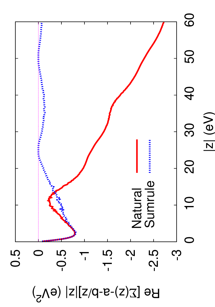
Figure 1: (color on-line) Deviation of the local $\Sigma(z)$ ($z=i\omega_{n}$) from the asymptotic form $\Sigma(z)\sim a+b/z$ for natural and sumrule boundary conditions. For natural boundary conditions the frequency independent part $a$ has an error.

We now discuss the FT for response functions, and use DCA as an illustration. The response function is calculated for a cluster in a bath. From the cluster response function vertex corrections are deduced. The Bethe-Salpeter equation for the lattice is then solved, assuming that the vertex corrections are the same as for the cluster. The embedded cluster problem is solved for imaginary time, while the Bethe-Salpeter equation is solved for imaginary frequency. The necessary FT to imaginary frequencies is numerically difficult.

We consider the electron-hole response function

$$\chi_{\sigma\sigma^{{}^{\prime}}}(q,k,k^{{}^{\prime}})=-{1\over\beta^{2}}\int_{0}^{\beta}d\tau_{1}\int_{0}^{\beta}d\tau_{2}\int_{0}^{\beta}d\tau_{3}\int_{0}^{\beta}d\tau_{4}$$

$$\times{\rm exp}\{-i[\omega_{n}\tau_{1}-(\omega_{n}+\nu)\tau_{2}+(\omega_{n^{{}^{\prime}}}+\nu)\tau_{3}-\omega_{n^{{}^{\prime}}}\tau_{4}]\}$$

$$\times\langle T_{\tau}[c^{\dagger}_{{\bf k}\sigma}(\tau_{1})c_{{\bf k+q}\sigma}(\tau_{2})c^{\dagger}_{{\bf k^{{}^{\prime}}+q}\sigma^{{}^{\prime}}}(\tau_{3})c_{{\bf k^{{}^{\prime}}}\sigma^{{}^{\prime}}}(\tau_{4})]\rangle,$$ (5)

with the compact notations $k=({\bf k},\omega_{n})$ and $q=({\bf q},\nu)$. Here $T_{\tau}$ is a time ordering symbol, $c^{\dagger}_{{\bf k}\sigma}$ creates an electron with wave vector ${\bf k}$ and spin $\sigma$ and $c(\tau)={\rm exp}(H\tau)c{\rm exp}(-H\tau)$, where $H$ is the Hamiltonian.

The $c$ operators are contracted pairwise and their expectation values are calculated. This is done for a very large number of configurations. It is convenient to perform the FT to imaginary frequency and reciprocal space for each configuration and to store the results in the $k$- and $q$-variables,Jarrell rather than storing the results in imaginary time and real space. We then need

$$g_{\sigma}(k,k^{{}^{\prime}})=\sum_{i=1}^{N_{\tau}}\sum_{j=1}^{N_{\tau}}\sum_{{\bf R}_{i}{\bf R}_{j}}e^{-i[\omega_{n}\tau_{i}-\omega_{n^{{}^{\prime}}}\tau_{j}]}$$ (6)

$$\times e^{i[{\bf k}\cdot{\bf R}_{i}-{\bf k^{{}^{\prime}}}\cdot{\bf R}_{j}]}\langle T_{\tau}[c^{\phantom{\dagger}}_{{\bf R}_{j}\sigma}(\tau_{j})c^{\dagger}_{{\bf R}_{i}\sigma}(\tau_{i})]\rangle(\Delta\tau)^{2},$$

where the integrals over $\tau$ have been replaced by sums over $N_{\tau}$ discrete values of $\tau$ separated by $\Delta\tau$ and ${\bf R}$ is a site index. Although this has the form of a Green’s function, it is calculated for a specific configuration and only the zeroth moment is known. This makes it harder to perform a FT. There is a singularity at $\tau_{i}=\tau_{j}$, which makes a straightforward spline in $\tau_{i}$ and $\tau_{j}$ less useful. The singularity can be handled by treating $\tau_{i}<\tau_{j}$ and $\tau_{i}>\tau_{j}$ separately. But a spline in two variables is still numerically very demanding because of the large number of points needed. To see this, we simplify the calculation in Eq. (6), by splitting it in two parts. Thus we calculate

$$f_{\sigma}(k,{\bf R}_{j},\tau_{j})=\sum_{i,{\bf R}_{i}}e^{-i(\omega_{n}\tau_{i}-{\bf k}\cdot{\bf R}_{i})}$$ (7)

$$\times\langle T_{\tau}[c_{{\bf R}_{j}\sigma}(\tau_{j})c^{\dagger}_{{\bf R}_{i}\sigma}(\tau_{i}))]\rangle,$$

and

$$g_{\sigma}(k,k^{{}^{\prime}})=\sum_{j,{\bf R}_{j}}e^{i(\omega_{n^{{}^{\prime}}}\tau_{j}-{\bf k^{{}^{\prime}}}\cdot{\bf R}_{j})}f_{\sigma}(k,{\bf R}_{j},\tau_{j}).$$ (8)

This gives

$$\chi_{\sigma\sigma^{{}^{\prime}}}(q,k,k^{{}^{\prime}})=-{1\over\beta^{2}}[g_{\sigma}(k+q,k)g_{\sigma^{{}^{\prime}}}(k^{{}^{\prime}},k^{{}^{\prime}}+q)$$

$$-g_{\sigma}(k^{{}^{\prime}},k)g_{\sigma}(k+q,k^{{}^{\prime}}+q)\delta_{\sigma\sigma^{{}^{\prime}}}](\Delta\tau)^{2}$$ (9)

Let the number of sites be $N_{c}$, the number of $\omega_{n}$-values $N_{\omega}$ and the number of $\nu$-values $N_{\nu}$. The number of ${\bf k}$-values is then also $N_{c}$. Let $N_{\tau}^{\rm c}$ be the number of $\tau$-points for which the correlation function in Eq. (7) is known and $N_{\tau}^{\rm s}$ the number of $\tau$-values needed to obtain an accurate FT. Eq. (7) and Eq. (8) then require of the order of $2(N_{\omega}+N_{\nu})N_{\tau}^{\rm c}N_{\tau}^{\rm s}N_{c}^{3}$ and $2(N_{\omega}+N_{\nu})^{2}N_{\tau}^{\rm s}N_{c}^{3}$ operations, respectively, for each configuration. Here we have assumed that the spline in the first $\tau$-variable is only done for each of the $N_{\tau}^{\rm c}$ values of the second $\tau$-variable. After the corresponding FT has been performed, the second variable is splined and FT. The calculations can easily be arranged so that the time needed for calculating the exponents is negligible and efficient machine routines can be used for the multiplications. Still, the calculations are very time consuming if $N_{\tau}^{\rm s}$ is large enough to give accurate FT. We therefore follow a different route, reducing the time requirement for Eqs (7, 8) very substantially and requiring no interpolation of the $\tau$-variables.

We first notice that

$$g_{{\sigma\bf R}_{i},{\bf R}_{j}}(\tau_{i},\tau_{j})=\langle[T_{\tau}c^{\phantom{\dagger}}_{{\bf R}_{j}\sigma}(\tau_{j})c^{\dagger}_{{\bf R}_{i}\sigma}(\tau_{i}))]\rangle$$ (10)

depends on $\tau_{i}$ and $\tau_{j}$ individually and not only on their difference, since it is calculated for one particular configuration. However, we can separate it as

$$g_{{\sigma\bf R}_{i}{\bf R}_{j}}(\tau_{i},\tau_{j})\equiv g^{0}_{{\sigma\bf R}_{i}{\bf R}_{j}}(\tau_{i}-\tau_{j})+\delta g_{{\sigma\bf R}_{i}{\bf R}_{j}}(\tau_{i},\tau_{j}),$$ (11)

where

$$g^{0}_{{\sigma\bf R}_{i}{\bf R}_{j}}(\tau_{i})={1\over N_{\tau}}\sum_{j=1}^{N_{\tau}}g_{{\sigma\bf R}_{i}{\bf R}_{j}}(\tau_{i+j-1},\tau_{j}),$$ (12)

only depends on one $\tau$-variable and we have defined $g_{{\sigma\bf R}_{i}{\bf R}_{j}}(\tau_{i+j-1},\tau_{j})=-g_{{\sigma\bf R}_{i}{\bf R}_{j}}(\tau_{i+j-1-N_{\tau}},\tau_{j})$ if $i+j-1>N_{\tau}$ or $g_{{\sigma\bf R}_{i}{\bf R}_{j}}(\tau_{i+j-1},\tau_{j})=-g_{{\sigma\bf R}_{i}{\bf R}_{j}}(\tau_{i+j-1+N_{\tau}},\tau_{j})$ $i+j-1<1$. Here, $g^{0}_{{\sigma\bf R}_{i}{\bf R}_{j}}(\tau_{i})$ is not a noninteracting Green’s function, but the time translationally invariant part of $g_{{\sigma\bf R}_{i}{\bf R}_{j}}(\tau_{i+j-1},\tau_{j})$. The singularities are now in $g^{0}_{{\sigma\bf R}_{i}{\bf R}_{j}}(\tau)$, and $\delta g_{{\sigma\bf R}_{i}{\bf R}_{j}}(\tau_{i},\tau_{j})$ is free of singularities, and can more easily be Fourier transformed.

Since $g^{0}_{{\sigma\bf R}_{i}{\bf R}_{j}}(\tau)$ only depends on one variable, it can easily be FT using a spline. Alternatively, we can use Filon’s rule,Abramowitz where second order polynomials are fitted to the $N_{\tau}$ $\tau$-points. These polynomials are then FT analytically. Even for $\omega_{n}\Delta\tau\gg 1$, the FT can be very accurate. This automatically gives the appropriate $1/(i\omega_{n})$ behavior for large $\omega_{n}$, due to end point corrections.

It is possible to FT $\delta g_{{\sigma\bf R}_{i}{\bf R}_{j}}(\tau_{i},\tau_{j})$ by performing a Filon’s rule for first $\tau_{i}$ and then for $\tau_{j}$. However, we have found it preferable to fit a two-dimensional polynomial

$$a_{00}+a_{10}\tau+a_{01}\tau^{\prime}+a_{11}\tau\tau^{\prime},$$ (13)

to the values of $\delta g_{{\sigma\bf R}_{i}{\bf R}_{j}}(\tau,\tau^{\prime})$ in the points $(\tau_{i},\tau_{j})$, $(\tau_{i+1},\tau_{j})$, $(\tau_{i},\tau_{j+1})$ and $(\tau_{i+1},\tau_{j+1})$. This is multiplied by the appropriate exponent and integrated analytically. Substantial simplification follow from the fact that $\delta g_{{\sigma\bf R}_{i}{\bf R}_{j}}(\tau,\tau^{{}^{\prime}})$ is antiperiodic and exp$[i(\omega_{n}\tau-\omega_{n^{{}^{\prime}}}\tau^{\prime}]\delta g_{{\sigma\bf R}_{i}{\bf R}_{j}}(\tau,\tau^{{}^{\prime}})$ is periodic in $\tau$ and $\tau^{\prime}$. Then

$$\int_{0}^{\beta}d\tau\int_{0}^{\beta}d\tau^{\prime}e^{i[\omega_{n}\tau-\omega_{n^{{}^{\prime}}}\tau^{\prime}]}\delta g_{{\sigma\bf R}_{i}{\bf R}_{j}}(\tau,\tau^{{}^{\prime}})=$$ (14)

$${1\over 4}c(\omega_{n},\omega_{n^{{}^{\prime}}},\Delta\tau/2)\sum_{i,j=1}^{N_{\tau}}e^{i[\omega_{n}\tau_{i}-\omega_{n^{{}^{\prime}}}\tau_{j}]}\delta g_{{\sigma\bf R}_{i}{\bf R}_{j}}(\tau_{i},\tau_{j}),$$

where $\tau_{i}=(i-1)\Delta\tau$ and $(N_{\tau}+1)\Delta\tau=\beta$. Here

$$c(x,y,\Delta)=$$

$$e^{-i\Delta(x-y)}[b_{0}^{x}b_{0}^{-y}+b_{0}^{x}b_{1}^{-y}+b_{1}^{x}b_{0}^{-y}+b_{1}^{x}b_{1}^{-y}]$$

$$e^{-i\Delta(x+y)}[b_{0}^{x}b_{0}^{-y}-b_{0}^{x}b_{1}^{-y}+b_{1}^{x}b_{0}^{-y}-b_{1}^{x}b_{1}^{-y}]$$

$$e^{i\Delta(x+y)}[b_{0}^{x}b_{0}^{-y}+b_{0}^{x}b_{1}^{-y}-b_{1}^{x}b_{0}^{-y}-b_{1}^{x}b_{1}^{-y}]$$

$$e^{i\Delta(x-y)}[b_{0}^{x}b_{0}^{-y}-b_{0}^{x}b_{1}^{-y}-b_{1}^{x}b_{0}^{-y}+b_{1}^{x}b_{1}^{-y}]$$

where

$$b_{0}^{x}=-{i\over x}(e^{ix\Delta}-e^{-ix\Delta})$$ (15)

$$b_{1}^{x}={1\over x^{2}\Delta}[e^{ix\Delta}(1-ix\Delta)-e^{-ix\Delta}(1+ix\Delta)]$$

This approach can easily be extended to the case of a nonuniform grid.

If $\delta g_{{\sigma\bf R}_{i}{\bf R}_{j}}(\tau,\tau^{{}^{\prime}})$ were a very smooth function, a more accurate integration method could be devised by fitting a polynomial of higher order. However, since $\delta g$ is obtained for a specific configuration, this does not seem useful.

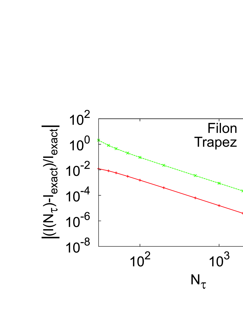
Figure 2: (color on-line) The relative accuracy of the FT of Eq. (16) according to the approach of Eq. (14) (Filon) or using the trapezoidal rule (Trapez).

To test the method, we have FT a function

$$f(\tau_{1},\tau_{2})=\sum_{ij}a_{ij}({\tau_{1}-\beta/2\over\beta/2})^{i}({\tau_{2}-\beta/2\over\beta/2})^{j},$$ (16)

where $a_{ij}$ is only nonzero for odd values of $i$ and $j$ to assure that the function is antiperiodic. Specifically, we chose $a_{11}=0.7$, $a_{13}=1.3$, $a_{15}=0.9$, $a_{31}=-1.2$, $a_{33}=1.5$, $a_{35}=-0.6$, $a_{51}=-0.8$, $a_{53}=1.1$, $a_{55}=-0.7$. We used the frequencies $\omega_{n}=13.5(2\pi/\beta)$ and $\omega_{n}^{{}^{\prime}}=9.5(2\pi/\beta)$, where $\beta=15$. Fig. 2 shows results obtained by using Eq. (14) (Filon) or the simple trapezoidal rule (Trapez). In the figure, the approach of Filon leads to a comparable accuracy as the trapezoidal rule for a $N_{\tau}$ that is almost one order of magnitude smaller.

In this Filon like approach the exponent is treated exactly and the error in the FT is entirely due to the limited information about the function to be FT. It is then no gain in adding extra points by interpolating the function to be FT. In a Hirsch-Fye approach this means that we put $N_{\tau}=N_{\tau}^{\rm c}$, the number of points determined by the discretization used.

From $\chi_{\sigma\sigma^{{}^{\prime}}i}(q,k,k^{{}^{\prime}})$ [Eq. (Fourier transformation and response functions)] we can calculate $\Pi(\tau)=\langle{\bf j}(\tau)\cdot{\bf j}(0)\rangle/(3N)$, where $N$ is the number of lattice sites and ${\bf j}$ is the current operator. The FT of $\Pi(\tau)$ is related to the optical conductivity $\sigma(\omega)$ via

$$\Pi(\nu)={1\over\pi}\int_{-\infty}^{\infty}{\omega^{2}\over\nu^{2}+\omega^{2}}\sigma(\omega)d\omega.$$ (17)

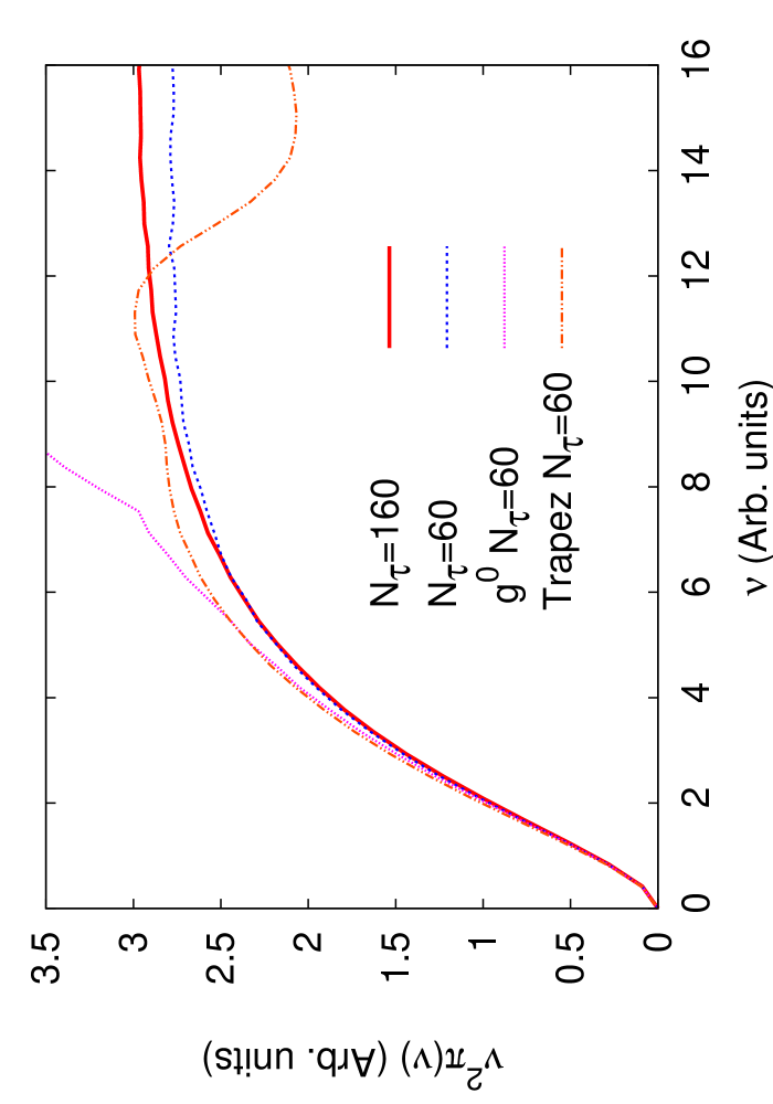
Figure 3: (color on-line)The quantity $\nu^{2}\Pi(\nu)$ as a function of $\nu$ for different values of $N_{\tau}$. The figure also shows results when $g^{0}$ has been split off [Eq. (11)] but the trapezoidal rule was used for $\delta g$ ($g^{0}$) or the total $g$ was integrated using a trapezoidal rule (Trapez).

Eq. (17) shows that $\nu^{2}\Pi(\nu)$ approaches a constant for large $\nu$. Problems of the FT should show up in particular for large $\nu$ and the accuracy should increase with $N_{\tau}$. We then choose $N_{\tau}$ so large that $\nu^{2}\Pi(\nu)$ is constant for large values of $\nu$-values. This should then be an accurate result.

Fig. 3 shows results for $\nu^{2}\Pi(\nu)$ for the 2d Hubbard model. The parameters are the same as in Fig. 1, except that $\beta=15$. The bath obtained for $N_{\tau}=160$ was used also for $N_{\tau}=60$. For $N_{\tau}=160$, $\nu^{2}\Pi(\nu)$ is constant for large $\nu$ over the whole range shown. The comparison with $N_{\tau}=60$ suggests that the FT is quite accurate at least for $\nu\Delta\tau\lesssim 2$ and it stays fairly accurate for substantially larger values $\nu\Delta\tau$. The deviation between $N_{\tau}=60$ and 160 could also be due to other inaccuracies for $N_{\tau}=60$ than the FT, and in that case the FT is accurate for even larger $\nu\Delta\tau$. The figure also shows a calculation where we split off $g^{0}$, [Eq. (11)], and FT it using Filon’s rule, but FT $\delta g$ using the trapezoidal rule ($g^{0}$ in the figure). We also performed the FT on the full $g$, without splitting off $g^{0}$, using the trapezoidal rule (Trapez in the figure). The figure shows that for $N_{\tau}^{\rm c}=60$ both approaches fail dramatically for large $\nu$.

To summarize, the FT of the Green’s function can be improved by using a spline with sumrule boundary conditions. This gives a $G(i\omega_{n})$ with correct first and second moments, while a natural spline in general gives an incorrect first moment. To calculate a response function, we need a FT a function $g(\tau_{i},\tau_{j})$ with a singularity. We show how a $g^{0}$ can be split off, which only depends on the difference $\tau_{i}-\tau_{j}$ and which contains the singularity. This function can be FT very accurately. For the rest, $\delta g$, we developed a two-dimensional FT in the spirit of Filon’s rule. This leads to accurate results, even if $g(\tau_{i},\tau_{j})$ is only known on a rather sparse mesh. ”After this paper had been submitted, an alternative prescription for efficient Fourier transforms of two-particle Green’s functions has been proposed by Kunes.Kunes

We would like to thank E. Gull, F. Assaad and A. Toschi for useful discussions and J. Bauer for a careful reading of the manuscript. One of us (G.S.) acknowledges support from the FWF under “Lise-Meitner” Grant No. M1136

References

• (1) T. Maier, M. Jarrell, T. Pruschke and M. H. Hettler, Rev. Mod. Phys. 77, 1027 (2005).
• (2) J. Hirsch and R. Fye, Phys. Rev. Lett. 56, 2521 (1986).
• (3) A.N. Rubtsov, V.V. Savkin, and A.I. Lichtenstein, Phys. Rev. B 72, 035122 (2005).
• (4) E. Gull, P. Werner, O. Parcollet and M. Troyer, EPL 82, 57003 (2008).
• (5) D.J. Luitz and F. Assaad, Phys. Rev. B 81, 024509 (2010).
• (6) P. Werner, A. Comanac, L. de’ Medici, M. Troyer, and A. J. Millis, Phys. Rev. Lett. 97, 076405 (2006).
• (7) See, e.g., N. Blümer, Ph. D. thesis, University of Augsburg, 2002.
• (8) A. Comanac, Ph.D. thesis, Columbia University (2007).
• (9) C. Knecht, Master thesis, Universität Mainz (2003).
• (10) E. Gull, Ph. D. thesis, DISS.ETH No. 18124 (2008).
• (11) A. Toschi, A. A. Katanin, and K. Held, Phys. Rev. B 75, 045118 (2007). A. Valli, G. Sangiovanni, O. Gunnarsson, A. Toschi, and K. Held, Phys. Rev. Lett. 104, 246402 (2010).
• (12) A. N. Rubtsov, M. I. Katsnelson, and A. I. Lichtenstein, Phys. Rev. B 77, 033101 (2008), S. Brener, H. Hafermann, A. N. Rubtsov, M. I. Katsnelson, and A. I. Lichtenstein, Phys. Rev. B 77, 195105 (2008).
• (13) J. K. Freericks, M. Jarrell and G.D. Mahan, Phys. Rev. Lett. 77, 4588 (1996).
• (14) P.J. Davis and I. Polonsky, in Handbook of Mathematical Functions, edited by M. Abramowitz and I.A. Stegun (Dover, NY,1970), p. 890.
• (15) J. Kunes (http://arxiv.org/abs/1010.3809).