Chiral Spin Textures of Strongly Interacting Particles in Quantum Dots

Abstract

We probe for statistical and Coulomb induced spin textures among the low-lying states of repulsively-interacting particles confined to potentials that are both rotationally and time-reversal invariant. In particular, we focus on two-dimensional quantum dots and employ configuration-interaction techniques to directly compute the correlated many-body eigenstates of the system. We produce spatial maps of the single-particle charge and spin density and verify the annular structure of the charge density and the rotational invariance of the spin field. We further compute two-point spin correlations to determine the correlated structure of a single component of the spin vector field. In addition, we compute three-point spin correlation functions to uncover chiral structures. We present evidence for both chiral and quasi-topological spin textures within energetically degenerate subspaces in the three- and four-particle system.

I Introduction

The investigation of correlations among electrons confined to quantum dots (QDs) is an active area of research in condensed matter physics due to their experimental tunability,Kouwenhoven et al. (2001); Bukowski and Simmons (2002) their theoretical efficacy,Reimann and Manninen (2002) and their application in, for example, quantum information science.Burkard (2006); Engel et al. (2004); Krenner et al. (2005); Taylor et al. (2005); Foletti et al. (2009); Laird et al. (2010) For two-dimensional QDs with circular confinement, the combination of confinement and long-range Coulomb repulsion results in charge densities peaked in annular regions about the dot center. Calculations of two-point correlation functionsGhosal et al. (2007) have further revealed that these confined electrons exhibit textures akin to Wigner molecules. Numerical work has shown these behaviors to depend on the size and shape of the quantum dot, as well as the strength of the applied magnetic field.Ghosal et al. (2006)

Since the spin of confined electrons provides a viable implementation of qubits,Loss and DiVincenzo (1998); Burkard et al. (1999) an understanding of the configurations and correlations formed among confined spins is crucial for the implementation of spin-qubits. Furthermore, the degree of control in fabrication and manipulation of QDs makes them ideal environments for the study of fundamental behaviors of both spin and charge. In this paper, we investigate the correlations that exist between the spins of electrons trapped in circular QDs. We are specifically interested in the formation of topological spin textures that may arise due to interaction or statistical effects among the confined charges.

A significant challenge in the development of spin-based quantum dot quantum computing is the suppression of decoherence of the spin-states for time-scales much longer than the time required to controllably flip a spin.Hanson et al. (2007); Ramsay (2010) The potential to encode information using topological degrees of freedom is appealing since the enhanced stability can mitigate the burden of error-correction. Various schemes which exploit a system’s topological structure have been proposed.Averin and Goldman (2001); Kitaev (2003); Das Sarma et al. (2005); Bombin and Martin-Delgado (2007) The advantage of these is that they are physically fault-tolerant; they are immune to local perturbations that degrade the coherent evolution of the state, a necessary ingredient in quantum computation.DiVincenzo (2000) Possible systems include two-dimensional spin modelsKitaev (2003) (for example, atoms in an optical latticeDuan et al. (2003)) and fractional quantum Hall systems.Das Sarma et al. (2005) These proposals rely on the existence of non-Abelian anyons in the excitation spectrum of the models for the information processing.

However, even in the absence of anyonic excitations, textures with topological structure are expected to be long-lived in-and-of-themselves due to their global correlations. Since correlations decrease decoherence,Bertoni et al. (2005); Climente et al. (2006, 2007) these topological structures could form an important processing element in more conventional quantum computing schemes. Even in finite-sized systems, where true topological stability likely does not occur, the relevant relaxation and decoherence times can be significantly enhanced. In Ref. Bertoni et al., 2005, for example, even moderate charge correlations were sufficient to more than double the decoherence time.

Numerical work has predicted the formation of spin textures in QDs immersed in a magnetic field.Governale (2002) Experimental evidence suggests the existence of fermionic spin textures in a two-dimensional electron gas (2DEG) confined in semiconductor heterostructures,Kumada et al. (2006) in vertical QDs,Nishi et al. (2006) and in few-electron lateral QDs.Ciorga et al. (2003); Sachrajda et al. (2004)

A topological spin qubit would be advantageous as it could be more robust against local environmental perturbations. Nuclear magnetic resonance measurements of GaAs/AlGaAs quantum wells have shown evidence for the localization of topological skyrmion spin textures as the temperature approaches 0 K.Khandelwal et al. (2001); Gervais et al. (2005) Recently, topological spin textures have been experimentally observed in topological insulators by means of spin-resolved angle-resolved photoemission spectroscopy.Hsieh et al. (2009) The emergence of a skyrmion lattice has also been detected in the chiral magnet MnSi using neutron scattering.Mühlbauer et al. (2009) Topological textures that are predicted to appear in QDs include vorticesSaarikoski et al. (2004); Tavernier, Anisimovas, and Peeters (2004); Saarikoski and Harju (2005); Yang et al. (2007); Anisimovas, Tavernier, and Peeters (2008) and merons.Yang et al. (2005); Petkovic and Milovanovic (2007); Milovanovic, Dobardzic, and Radovic (2009) Vortices occur in the presence of a strong external magnetic field, when electron current circulates in a plane around localized regions of low electron density. Merons are topological spin textures characterized by a central “up” or “down” spin which smoothly transitions into an in-plane 2$\pi$-winding along its boundary.Moon et al. (1995) As developed in the theory, the realization of both types of quasiparticles requires the presence of an external magnetic field.

In this work, we present evidence for the existence of spin textures in circular QDs for both three-electron and four-electron systems in the absence of an external magnetic field. The electronic wave functions are calculated by configuration interaction techniques. Two-point and three-point spin correlations are calculated in order to uncover both correlation and chirality in the spin textures which are concealed in superpositions of different configurations.

In Sec. II, we introduce our model and the foundation upon which our calculations are based. Section III describes specifically the spin correlation calculations used to examine the spin textures in the QD. We then go on to describe our results for systems of three (Sec. IV) and four (Sec. V) interacting particles. We conclude with a summary of our findings, their implications, and suggestions for further investigations in Sec. VI.

II Quantum Dot System

Our system consists of $N$ interacting quasiparticles of charge $e$, bound to a two-dimensional (2D) plane and laterally confined by a parabolic potential. The 2D Hamiltonian used to describe this “standard model” is

$$\hat{\mathcal{H}}=\sum_{i}^{N}\hat{h}_{i}+\frac{1}{2}\sum_{i\neq j}^{N}\frac{e^{2}}{\epsilon|\hat{\boldsymbol{{r}}}_{i}-\hat{\boldsymbol{{r}}}_{j}|},$$ (1a)

where $$\epsilon \hat{h}$$ is the dielectric constant of the medium and is the single-particle Hamiltonian describing harmonic confinement;

$$\hat{h}=\frac{1}{2m^{*}}\left(\hat{\boldsymbol{{p}}}+\frac{e}{c}\widehat{\boldsymbol{{A}}}\left(\hat{\boldsymbol{{r}}}\right)\right)^{2}+\frac{1}{2}m^{*}\omega_{0}^{2}\hat{r}^{2},$$ (1b)

where $m^{*}$ is the effective mass, $\hat{\boldsymbol{{r}}}=(\hat{x},\hat{y})$ the position operator, and $\omega_{0}$ the parabolic confinement frequency. Throughout this paper, we take the magnetic field to be zero, and therefore set the vector potential $\widehat{\boldsymbol{{A}}}\left(\hat{\boldsymbol{{r}}}\right)=0$.

Two harmonic-oscillator quantum numbers, $n,m=0,1,2,\ldots$, characterize the eigenstates of the single-particle Hamiltonian,Jacak et al. (1997) Eq. (1b). These eigenstates are the “atomic orbitals” of the QD, and are given by

$$\left|{nm}\right\rangle=\frac{1}{\sqrt{n!m!}}(a^{\dagger})^{n}(b^{\dagger})^{m}\left|{00}\right\rangle,$$ (2)

where, $a^{\dagger}$ and $b^{\dagger}$ are the usual Bose creation operators, and $\left|{00}\right\rangle$ is the single-particle ground state. These orbitals have energy $\varepsilon_{nm}$ given by

$$\varepsilon_{nm}=\hbar\Omega_{+}(n+\tfrac{1}{2})+\hbar\Omega_{-}(m+\tfrac{1}{2}),$$ (3)

where $\Omega_{\pm}=(\sqrt{4\omega_{0}^{2}+\omega_{c}^{2}}\pm\omega_{c})/2$, and $\omega_{c}=e\boldsymbol{{B}}/(m^{*}c)$ is the cyclotron frequency. This energy reduces to $\hbar\,\omega_{0}(n+m+1)$ in the absence of a magnetic field.

The single-particle Hamiltonian, the $z$-component of the orbital angular momentum, $\hat{L}_{z}$, and a component of the spin operator—which we take to be the $z$-component $\hat{S}_{z}$—form a set of commuting observables which we take to classify our states: $\hat{L}_{z}|nms\rangle=\hbar(n-m)|nms\rangle$, $\hat{S}_{z}|nms\rangle=\hbar s|nms\rangle$, $\hat{h}|nms\rangle=\varepsilon_{nm}|nms\rangle$.

We are interested in spatial textures formed by the spin field, and so we require the position-space representation of the orbitals.Jacak et al. (1997) These are given byorb

$$\phi_{nm}(r,\theta)=(-1)^{n_{r}}\frac{1}{\sqrt{2\pi}l_{0}}\sqrt{\frac{n_{r}!}{\left(n_{r}+|m^{\prime}|\right)!}}\\ \times e^{im^{\prime}\theta}e^{-r^{2}/(4l_{0}^{2})}\left(\frac{r}{\sqrt{2}l_{0}}\right)^{|m^{\prime}|}L_{n_{r}}^{|m^{\prime}|}\left(\frac{r^{2}}{2l_{0}^{2}}\right),$$ (4)

where $r$ and $\theta$ are the polar coordinates in two dimensions, $l_{0}=\sqrt{\hbar/(2m^{*}\omega)}$ is the effective length with $\omega=\sqrt{4\omega_{0}^{2}+\omega_{c}^{2}}/2$, $n^{\prime}=n+m$, $m^{\prime}=n-m$, $n_{r}=(n^{\prime}-|m^{\prime}|)/2$, and $L_{n}^{(\alpha)}(x)$ is the generalized Laguerre polynomial.Abramowitz and Stegun (1965)

The eigenstates of the interacting system are determined by exact diagonalization of Eq. (1a). This procedure begins by determining many-particle basis states (Slater determinants), eigenstates of Eq. (1b), that are composed of antisymmetrized products of the single-particle states in Eq. (2). We use 288 single-particle states, and as many as 4900 many-particle basis states in the diagonalization routine. Without loss of fidelity, and for computational efficiency, the number of many-particle basis states is reduced when determining the two-point and three-point spin correlation calculations over the range of the entire QD. Block-diagonalization is performed for a given set of parameters. These include system parameters ($B$, $\omega_{0}$, $m^{*}$, $\epsilon$) and the conserved quantities $N$, $L_{z}$, $S_{z}$, $S^{2}$. The Coulomb matrix elements are evaluated using the convenient closed-form expression derived in Ref. Kyriakidis et al., 2002.

With the eigenstates determined, we calculate one-, two-, and three-point position-dependent spin correlation functions over energetically-degenerate manifolds. The structure of the particular operators used in these calculations is discussed in the next section.

III Product Spin Operators

For our investigation, we require the products of up to three one-body spin operators. Here, we introduce the product-operators used in the calculations shown in the proceeding sections. The details associated with the derivation of each product-operator are discussed in the Appendix.

III.1 One-Body Spin Operators

Except where indicated, all averages are taken over energetically-degenerate manifolds. That is to say,

$$\langle A\rangle=\frac{\text{Tr}(\hat{\rho}\,\hat{A})}{\text{Tr}(\hat{\rho})},$$ (5a)

where the density operator $$\hat{\rho}$$ is defined as

$$\hat{\rho}=\sum_{i=1}^{n}\left|{E_{i}}\right\rangle\left\langle{E_{i}}\right|,$$ (5b)

and where the states $|E_{i}\rangle$ are all the states in a given degenerate manifold of Eq. (1): $\hat{{\cal H}}|E_{i}\rangle=\text{const.}\,|E_{i}\rangle$ for all $i=1,2,\ldots n$.

Our analysis begins with the evaluation of both spin density and number density at position $\boldsymbol{{r}}$ in the QD system. We are specifically interested in isolating the spin-up and spin-down densities along the coordinate axes. Due to the conservation of spin in the system, these one-body spin operators can only distinguish the spin-up density from the spin-down density along a single axis. We therefore define a set of spin operators $\hat{S}_{\pm z}(\boldsymbol{{r}})$ that separately determines the spin-up and spin-down densities along $z$ at position $\boldsymbol{{r}}$. In canonical form (see Appendix Eq. (16)), this is given by

$$\hat{S}_{s\,z}(\boldsymbol{{r}})=\sum_{i\,j}U_{ijs}\hat{c}_{is}^{\dagger}\hat{c}_{js}^{\phantom{\dagger}},$$ (6)

where $U_{ijs}=s\phi_{i}^{*}(\boldsymbol{{r}})\phi_{j}(\boldsymbol{{r}})/2$, with $s=\pm 1$ ($\hbar=1$). Note the composite indexes $i$ and $j$ each represent a set of orbital quantum numbers $n$ and $m$.

The number density and spin density operators at position $\boldsymbol{{r}}$ are then given by

$$\hat{n}(\boldsymbol{{r}})=\sum_{s}\hat{\psi}_{s}^{\dagger}(\boldsymbol{{r}})\hat{\psi}_{s}^{\phantom{\dagger}}(\boldsymbol{{r}})=2\left(\hat{S}_{+z}(\boldsymbol{{r}})+\hat{S}_{-z}(\boldsymbol{{r}})\right),$$ (7)

$$\hat{S}_{z}(\boldsymbol{{r}})=\frac{1}{2}\sum_{s}s\hat{\psi}_{s}^{\dagger}(\boldsymbol{{r}})\hat{\psi}_{s}^{\phantom{\dagger}}(\boldsymbol{{r}})=\left(\hat{S}_{+z}(\boldsymbol{{r}})-\hat{S}_{-z}(\boldsymbol{{r}})\right),$$ (8)

where $\hat{\psi}_{s}^{\dagger}(\boldsymbol{{r}})$ and $\hat{\psi}_{s}(\boldsymbol{{r}})$ are field operators that respectively create and annihilate a fermion at position $\boldsymbol{{r}}$, with spin $s$. In terms of the eigenstates $|nms\rangle$ of Eq. (1b), the field operators are given by

$$\hat{\psi}_{s}^{\dagger}(\boldsymbol{{r}})=\sum_{n\,m}\phi_{nm}^{*}(\boldsymbol{{r}})\hat{c}_{nms}^{\dagger},$$ (9)

with $\phi_{nm}(\boldsymbol{{r}})=\langle\boldsymbol{{r}}|nm\rangle$ given in Eq. (4).

The effects of Coulomb interaction between the particles are apparent when the expectation values of the above operators are compared between the interacting and noninteracting systems.

III.2 Two-Body Spin Operators

We next investigate the two-point correlations as projected onto the $z$-axis. (Any other choice yields identical results.) Unless otherwise indicated, a spin-up (spin-down) particle refers to a particle with spin polarized along the positive (negative) axis of quantization (in this work, the $z$-axis). Specifically, we investigate $\langle S_{+z}(\boldsymbol{{r}}_{0})S_{+z}(\boldsymbol{{r}}_{1})\rangle$ and $\langle S_{+z}(\boldsymbol{{r}}_{0})S_{-z}(\boldsymbol{{r}}_{1})\rangle$. In canonical form, the operators are given by

$$\hat{S}_{+z}(\boldsymbol{{r}}_{0})\hat{S}_{\sigma z}(\boldsymbol{{r}}_{1})=\frac{1}{2}\sum_{ijklss^{\prime}}Q_{ijkl}^{ss^{\prime}\sigma}\hat{c}_{is}^{\dagger}\hat{c}_{js^{\prime}}^{\dagger}\hat{c}_{ls^{\prime}}\hat{c}_{ks},$$ (10a)

with

$$Q_{ijkl}^{ss^{\prime}\sigma}=\frac{1}{4}\left(\phi_{i}^{*}(\boldsymbol{{r}}_{0})\phi_{j}^{*}(\boldsymbol{{r}}_{1})\phi_{k}(\boldsymbol{{r}}_{0})\phi_{l}(\boldsymbol{{r}}_{1})\delta_{s\uparrow}\delta_{s^{\prime}\sigma}\right.\\ \left.\mbox{}+\phi_{j}^{*}(\boldsymbol{{r}}_{0})\phi_{i}^{*}(\boldsymbol{{r}}_{1})\phi_{l}(\boldsymbol{{r}}_{0})\phi_{k}(\boldsymbol{{r}}_{1})\delta_{s\sigma}\delta_{s^{\prime}\uparrow}\right),$$ (10b)

and $\sigma=\pm 1$. As in Eq. (6), the indexes $i$ through $l$ in Eq. (10) are again composite indexes of pairs of orbital quantum numbers. The two-point spin correlations measure the probability of finding a particle with spin projection $\sigma z$ at position $\boldsymbol{{r}}_{1}$ given the existence of a particle with spin projection $+z$ at position $\boldsymbol{{r}}_{0}$.

Finally, the correlation between a spin-up particle at $\boldsymbol{{r}}_{0}$ and the net spin density at $\boldsymbol{{r}}_{1}$ is

$$\hat{S}_{+z}(\boldsymbol{{r}}_{0})\hat{S}_{\text{net }z}(\boldsymbol{{r}}_{1})\\ =\hat{S}_{+z}(\boldsymbol{{r}}_{0})\hat{S}_{+z}(\boldsymbol{{r}}_{1})-\hat{S}_{+z}(\boldsymbol{{r}}_{0})\hat{S}_{-z}(\boldsymbol{{r}}_{1}).$$ (11)

These two-point spin correlations are useful for determining parallel or antiparallel spin properties such as magnetic ordering.Ghosal et al. (2007) They are insufficient, however, for determining chiral textures where correlations are measured with respect to orthogonal axes. For that we turn to the three-point spin correlation functions next.

III.3 Three-Body Spin Operators

We compute three unique three-point correlations:

$$\left\langle S_{+x}(\boldsymbol{{r}}_{0})S_{+y}(\boldsymbol{{r}}_{1})S_{\text{net}\;x}(\boldsymbol{{r}}_{2})\right\rangle,$$ (12a)

$$\left\langle S_{+x}(\boldsymbol{{r}}_{0})S_{+y}(\boldsymbol{{r}}_{1})S_{\text{net}\;y}(\boldsymbol{{r}}_{2})\right\rangle,$$ (12b)

and

$$\left\langle S_{+x}(\boldsymbol{{r}}_{0})S_{+y}(\boldsymbol{{r}}_{1})S_{\text{net}\;z}(\boldsymbol{{r}}_{2})\right\rangle.$$ (12c)

These three-point spin correlations measure the probability of finding a particle with spin projected along the $x$, $y$ or $z$ axis, respectively, given there is a particle at position $\boldsymbol{{r}}_{0}$ that is spin-up along the $x$-axis and a particle at position $\boldsymbol{{r}}_{1}$ that is spin-up along the $y$-axis. Whereas the two-point functions can determine whether the spin-projection of a second particle is parallel or antiparallel to the spin-projection of the first particle, it cannot determine the orientation of the spin of the second particle in a plane other than that of the spin of the first particle. The three-point functions in Eq. (12) can indeed uncover such chiral structure. Explicitly, the three-body spin operators can be expressed as

$$\hat{S}_{+x}(\boldsymbol{{r}}_{0})\hat{S}_{+y}(\boldsymbol{{r}}_{1})\hat{S}_{\text{net}\;x}(\boldsymbol{{r}}_{2})\\ =\frac{1}{3!}\sum_{\begin{subarray}{c}ijklmn\\ s_{{}_{1}}s_{{}_{2}}s_{{}_{3}}\end{subarray}}K_{ijklmn}^{s_{{}_{1}}s_{{}_{2}}s_{{}_{3}}}\hat{c}_{is_{{}_{1}}}^{\dagger}\hat{c}_{js_{{}_{2}}}^{\dagger}\hat{c}_{ks_{{}_{3}}}^{\dagger}\hat{c}_{ns_{{}_{3}}}^{\phantom{\dagger}}\hat{c}_{ms_{{}_{2}}}^{\phantom{\dagger}}\hat{c}_{ls_{{}_{1}}}^{\phantom{\dagger}},$$ (13a)

where

$$K_{ijklmn}^{s_{{}_{1}}s_{{}_{2}}s_{{}_{3}}}=\frac{3}{16}\delta_{s_{{}_{1}}s_{{}_{2}}}\delta_{s_{{}_{2}}\bar{s}_{{}_{3}}}\\ \times\left[is_{3}\phi_{i}^{*}(\boldsymbol{{r}}_{0})\phi_{j}^{*}(\boldsymbol{{r}}_{1})\phi_{k}^{*}(\boldsymbol{{r}}_{2})\phi_{m}(\boldsymbol{{r}}_{0})\phi_{n}(\boldsymbol{{r}}_{1})\phi_{l}(\boldsymbol{{r}}_{2})\right.\\ \mbox{}-i\phi_{i}^{*}(\boldsymbol{{r}}_{0})\phi_{k}^{*}(\boldsymbol{{r}}_{1})\phi_{j}^{*}(\boldsymbol{{r}}_{2})\phi_{m}(\boldsymbol{{r}}_{0})\phi_{l}(\boldsymbol{{r}}_{1})\phi_{n}(\boldsymbol{{r}}_{2})\\ \mbox{}-\phi_{i}^{*}(\boldsymbol{{r}}_{0})\phi_{j}^{*}(\boldsymbol{{r}}_{1})\phi_{k}^{*}(\boldsymbol{{r}}_{2})\phi_{n}(\boldsymbol{{r}}_{0})\phi_{m}(\boldsymbol{{r}}_{1})\phi_{l}(\boldsymbol{{r}}_{2})\\ \left.\mbox{}-\phi_{k}^{*}(\boldsymbol{{r}}_{0})\phi_{i}^{*}(\boldsymbol{{r}}_{1})\phi_{j}^{*}(\boldsymbol{{r}}_{2})\phi_{m}(\boldsymbol{{r}}_{0})\phi_{l}(\boldsymbol{{r}}_{1})\phi_{n}(\boldsymbol{{r}}_{2})\right],$$ (13b)

and with similar expressions for the remaining two operators in Eq. (12). In Eq. (13), each of the six indexes $i$ through $n$ is once again a composite index over pairs of orbital quantum numbers. Furthermore, in Eq. (13b), $\bar{s}_{i}\equiv-s_{i}$, with $s_{i}=\pm 1$ denoting the usual spin projections.

The choice for the first two spin-projections is not unique; due to the absence of a preferred spin orientation in the system, each expression is equivalent to any cyclic permutation of the spin components. We focus below on the cases where two of the three spins operators lie in the ($x$-$y$) plane of the dot.

IV Three-Particle System

In this section, we investigate spin correlations that exist in the two lowest-lying states of a system with three charged particles. Our system is modeled with GaAs parameters ($\epsilon=12.4$ and $m^{*}=0.067m_{e}$), and our confinement potential is $\omega_{0}=1.0$ meV, yielding an effective length at $B=0$ of $l_{0}=23.8$ nm.

IV.1 Ground State Manifold

At zero magnetic field, the ground state of the three-particle system is four-fold degenerate, with quantum numbers $L_{z}=\pm 1$, $S=1/2$, and $S_{z}=\pm 1/2$. We compute $\langle S_{+z}(\boldsymbol{{r}})\rangle$ and $\langle S_{-z}(\boldsymbol{{r}})\rangle$ within this degenerate subspace. [See Eq. (5).] From these, we determine both the net density, $\langle n(\boldsymbol{{r}})\rangle$, Eq. (7), and the net spin $\langle S_{z}(\boldsymbol{{r}})\rangle$, Eq. (8). We then go on to calculate the two-point spin functions to demonstrate correlations between parallel and antiparallel spin components, followed by the three-point functions to uncover chiral correlations.

IV.1.1 Single-particle densities

To illustrate the effects of long-range Coulomb repulsions, we consider the spin density with and without interactions. In the non-interacting case, each eigenstate is a single antisymmetrized orbital configuration. For the three-particle system, there are two particles on the $|nm\rangle=|00\rangle$ orbital, and one on either the $|10\rangle$ or $|01\rangle$ orbital. This yields four degenerate states with quantum numbers $(S,S_{z},L_{z})=(1/2,\pm 1/2,\pm 1)$. For the interacting case, these symmetries are not explicitly broken; the degeneracy and the quantum numbers remain the same, but the states themselves are now correlated, involving many other orbital configurations consistent with the symmetry.

Figure 1 shows single-particle densities for the total ground-state manifold as a function of radial distance from the center for both the interacting and non-interacting cases.

Figure 1: (Color online.) Radial dependence of the single-particle spin and number density in the three-particle ground state manifold. Inset shows densities in absence of Coulomb interaction. (Inset axes have the same dimensions as the main plot).

There is azimuthal symmetry for these configurations due to the underlying circular symmetry of the dot itself, manifest in the Hamiltonian, Eq. (1).

The non-interacting case is characterized as Gaussian-like with a peak at the origin. When Coulomb interactions are considered, the repulsion smears out the density over different orbital configurations.Stevenson and Kyriakidis (2011) The competition between repulsion and confinement results in an annular density about the origin. These interaction effects are strong; the ground-state energy of the interacting system is 10.30 meV for these experimentally-relevant system parameters—more than twice the ground-state energy of the non-interacting case (4.0 meV).

The effects of Coulomb repulsion are also reflected in the single-particle spin densities as well. Note, however, that in both cases we have $\langle S_{+z}(\boldsymbol{{r}})\rangle=\langle S_{-z}(\boldsymbol{{r}})\rangle$: $\langle S_{\text{net }z}(\boldsymbol{{r}})\rangle=0$ everywhere in the dot, therefore the one-point calculations are insufficient for showing the Coulomb effects on spin. This is a consequence of the SU(2) symmetry present at zero magnetic field.

IV.1.2 Two-point spin correlations

For the two-point spin correlations, Eq. (10), we consider the case where $\boldsymbol{{r}}_{0}$ is fixed at the location of maximum single-particle density, $r_{\text{max}}\equiv 39$ nm, as obtained in the previous section. We further define the angular location of $\boldsymbol{{r}}_{0}$ to be $\theta_{0}=0$. We do not the discuss the non-interacting limit for these calculations.

The two-point correlations $\langle S_{+z}(\boldsymbol{{r}}_{0})S_{+z}(\boldsymbol{{r}}_{1})\rangle$ and $\langle S_{+z}(\boldsymbol{{r}}_{0})S_{-z}(\boldsymbol{{r}}_{1})\rangle$ for the interacting ground-state manifold are shown in Fig. 2 as a function of $\boldsymbol{{r}}_{1}$ for $\boldsymbol{{r}}_{0}=(r_{\text{max}},\theta_{0})$.

Figure 2: (Color online.) Two-point spin correlation functions for the three-particle ground state manifold. Distributions are shown for the spin-up (a) and spin-down (b) densities at $\boldsymbol{{r}}_{1}$ given a spin-up particle at $\boldsymbol{{r}}_{0}=(39~{}\text{nm},\,0)$, denoted by a cross.

Two peaks are evident along the ring of radius $r_{\text{max}}$. Note that our averages, Eq. (5), are obtained by tracing over all the degenerate states in the ground-state manifold. An incipient Wigner crystallization is apparent with the spins forming a classical-like lattice at the vertexes of a triangle.Ghosal et al. (2006, 2007) This structure is not seen in the non-interacting case, implying that the Coulomb repulsion between the particles is responsible for this spin texture.

To more clearly probe the angular inhomogeneity, we plot in Fig. 3 results along the ring $r_{\text{max}}$.

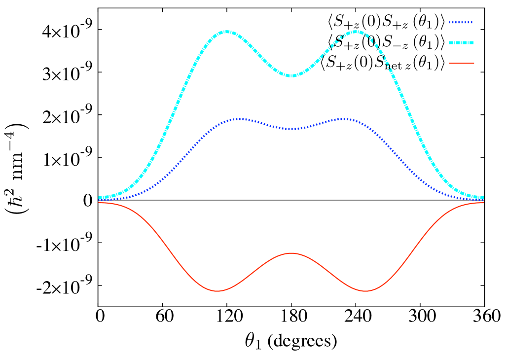
Figure 3: (Color online.) Trace along $r_{\text{max}}=39$ nm in the three-particle ground state manifold, revealing the spin distribution with respect to a spin-up particle at $\boldsymbol{{r}}_{0}=(r_{\text{max}},0)$.

In particular, we show the net spin $S_{z}$ as well as the individual components $S_{\pm z}$, given a spin-up particle at $\boldsymbol{{r}}_{0}$. Note as $\boldsymbol{{r}}_{1}$ approaches $\boldsymbol{{r}}_{0}$ the remaining spin-up density goes to zero, indicative of a Pauli vortexSaarikoski et al. (2010) at that position. As well, the spin density at the two peaks is not fully polarized, indicating a degree of canting away from the $z$-axis: The net spin tilts towards the $x$-$y$ plane. The lack of equal magnitudes of spin-up and spin-down probabilities at every point along $r_{\text{max}}$ in Fig. 3 indicates that the spin density never lies completely in the $x$-$y$ plane. Since the spin-density never crosses through the plane, it cannot have winding order. Windings are important in these spin systems as they represent clear examples of topologically stable structures.

The two-point correlations are insufficient to determine the probable orientation of the spin in the x-y plane, so the results of these calculations can be interpreted as the smearing out of the net spin across the surface of a cone centred at a local z-axis at every point measured in the calculation. The opening angle of the cone is twice that of the local canting angle, the degree of tilting from the local z-axis, of the spin. This cone, along with the canting angle, is illustrated in Fig. 4.

Figure 4: (Color online.) Canting angle $\alpha$ with respect to the axis of quantization (the $z$ axis). The spin is not fully polarized along either the $+z$ or $-z$ axis but has components of both projections, thus smearing out along a cone of probability about the z-axis.

The canting angle can be determined in the following manner: If we consider the spin density field shown in Fig. 3 as itself a spin-half field, we may generally write its local orientation as

$$\left|\psi(r_{\text{max}},\theta_{1})\right\rangle=\frac{1}{N}\left(c_{+}|+z\rangle+\text{e}^{i\beta}c_{-}|-z\rangle\right),$$ (14)

where $c_{\pm}$ are real and may be defined as

$$c_{+}=\left\langle S_{+z}(\boldsymbol{{r}}_{0})S_{+z}(r_{\text{max}},\theta_{1})\right\rangle\equiv N\cos\frac{\alpha}{2},$$ (15a)

$$c_{-}=\left\langle S_{+z}(\boldsymbol{{r}}_{0})S_{-z}(r_{\text{max}},\theta_{1})\right\rangle\equiv N\sin\frac{\alpha}{2},$$ (15b)

and where $N=\sqrt{c_{+}^{2}+c_{-}^{2}}$ is a local normalization. The symmetry of the two-point functions prevents discrimination of different values of the azimuthal angle $\beta$, but it can determine the canting angle $\alpha$.

For each of the two peaks in Fig. 3, the canting angle with respect to the positive $z$-axis is determined to be $\alpha=131^{\circ}$. That is, relative to a spin-up particle at $\boldsymbol{{r}}_{0}$, the spin-density peaks describing the other two particles both occupy the surface of a cone with canting angle 49^∘ from the negative $z$-axis. Figure 5 shows the resulting canting angle from the positive $z$-axis of the local Bloch vector for each value of $\theta_{1}$ along the ring $r_{\text{max}}$. The canting angle becomes greatest ($\alpha$ approaches $180^{\circ}$) as $\theta_{1}$ approaches $\theta_{0}$ = 0, and is a minimum at $\theta_{1}=180^{\circ}$. (Pauli exclusion dictates that $\alpha\rightarrow 180^{\circ}$ as $\theta_{1}\rightarrow\theta_{0}$.)

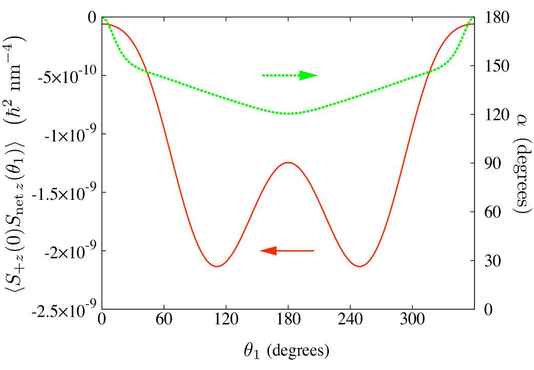
Figure 5: (Color online.) Canting angle $\alpha$ as a function of $\theta_{1}$ along the ring of maximum single-particle density $r_{\text{max}}$ = 39 nm in the three-particle ground state manifold. The net spin density from the two-point calculation along the same ring $r_{\text{max}}$ is shown for reference.

The two-point functions in this system with SU(2) symmetry are insufficient to distinguish chiral structures. Three-point functions are necessary to resolve spin components in the plane perpendicular to the axis defined by the two-point functions. We turn to these next.

IV.1.3 Three-point spin correlations

As described in Sec. III.3, we compute the three distinct three-point correlation functions given in Eq. (12). Other three-point functions can be related to one of these three due to the symmetry of the underlying Hamiltonian.

In Eq. (12), we fix $\boldsymbol{{r}}_{0}$ on the ring of maximum single-particle density ($r_{\text{max}}$ = 39 nm) at $\theta_{0}$ = 0. The correlation functions are then a function of the four variables $r_{1}$, $\theta_{1}$, $r_{2}$, and $\theta_{2}$. If we further choose to probe the system along the ring $r_{\text{max}}$, we then obtain the two-dimensional map in the two angles $\theta_{1}$ and $\theta_{2}$ shown in Fig. 6(a).

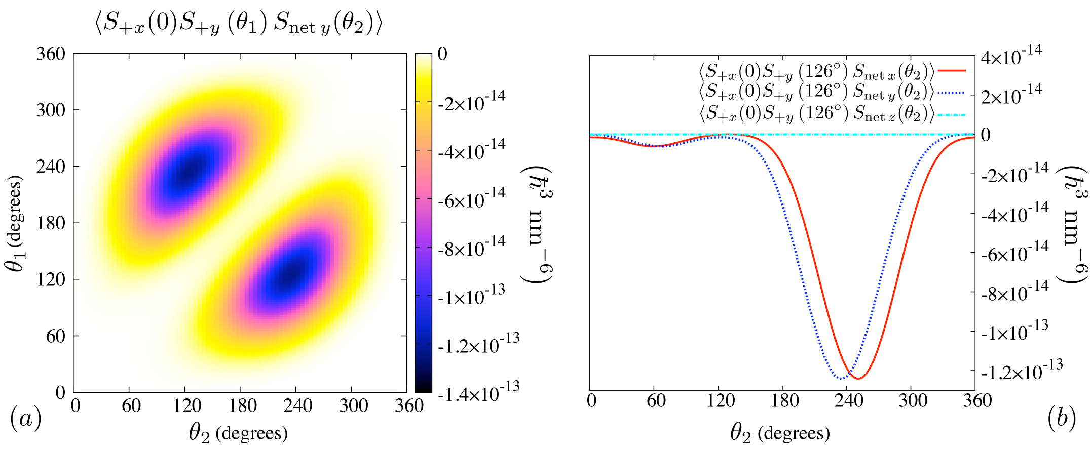
Figure 6: (Color online.) Three-point spin correlations, Eq. (12), along the ring $r_{\text{max}}=39$ nm for the three-particle ground state manifold. (a) The net $S_{y}$ is plotted given a spin-up particle along the $x$-axis at $\theta_{0}=0^{\circ}$ and a spin-up particle along the $y$-axis at $\theta_{1}$. (b) The three-point correlations for net spins along the $x$, $y$ and $z$ axes for $\theta_{0}=0^{\circ}$ and $\theta_{1}=126^{\circ}$ on the ring $r_{\text{max}}$.

Explicitly, Fig. 6(a) is a plot of $\langle S_{+x}(r_{\text{max}},\,0)S_{+y}(r_{\text{max}},\theta_{1})S_{\text{net}\ y}(r_{\text{max}},\theta_{2})\rangle$ as a function of $\theta_{1}$ and $\theta_{2}$. As the angular location of the second spin approaches $\theta_{1}=120^{\circ}$ with respect to the first spin, a peak emerges in the net spin distribution along the $y$-axis. The maximum correlations occur at $(\theta_{1},\theta_{2})=(126^{\circ},235^{\circ})$ and $(234^{\circ},125^{\circ})$. Note the inversion symmetry about the point $(180^{\circ},180^{\circ})$. Very similar results are seen for the net spin distribution along the $x$-axis (not shown).

The three-point correlations for the net spin distributions along the $x$, $y$ and $z$ axes with respect to a spin-up particle along the $x$-axis at $\boldsymbol{{r}}_{0}=(r_{\text{max}},0)$, and a spin-up particle along the $y$-axis at $\boldsymbol{{r}}_{1}=(r_{\text{max}},126^{\circ})$ are displayed in Fig. 6(b). Note the net spin distribution along the $z$-axis is negligible in comparison to the distributions along the $x$ and $y$ axes: Any spin density that remains in the system lies only in the plane of the two spins at $\boldsymbol{{r}}_{0}$ and $\boldsymbol{{r}}_{1}$, respectively.

Figure 7 is a map of the net spin distribution in the three-particle ground-state manifold, given a spin-up particle along $x$ at $\boldsymbol{{r}}_{0}=(r_{\text{max}},\,0)$ and a spin-up particle along $y$ at $\boldsymbol{{r}}_{1}=(r_{\text{max}},126^{\circ})$.

Figure 7: (Color online.) Net spin distribution in the plane of the QD for the three-particle ground state manifold, as determined by three-point spin correlations. The magnitude is denoted by the color bar and the direction is indicated by the vector field. The $z$-component is negligible here. The calculation is done with respect to a particle of spin-up projection on the $x$-axis at $\boldsymbol{{r}}_{0}=(39~{}\text{nm},0^{\circ})$ and a particle of spin-up projection on the $y$-axis at $\boldsymbol{{r}}_{1}=(39~{}\text{nm},126^{\circ})$. (These locations are denoted by the blue arrows.

The peak along the ring $r_{\text{max}}$ occurs at $\theta_{3}=243^{\circ}$, and the net spin at this peak has an equal spin-down projection along each the $x$ and $y$ axes. Note in this distribution the peak of the net spin density and the two locations $\boldsymbol{{r}}_{0}$ and $\boldsymbol{{r}}_{1}$ are each equidistant from each other.

The three-point correlations suggest that the most probable spin configuration in this three-particle state has a planar, splayed order, as seen in Fig. 7. Recall, however, that the results from the two-point correlations imply that the state does not have a clear winding order.

IV.2 First Excited State

Like the three-particle ground state, the first excited state is also four-fold degenerate. However, in contrast to the ground state manifold, $L_{z}=0$ for all four degenerate states in the first excited state. Degeneracy occurs through the spin quantum numbers $S=3/2$, and $S_{z}=\pm 3/2,\ \pm 1/2$.

As in the ground state, the single-particle density and the spin density distributions are rotationally symmetric. When interactions are considered, the annular distributions peak at $r_{\text{max}}\equiv 41$ nm. These distributions are similar to those seen in Fig. 1 for the ground state and are not shown. As seen in the ground state manifold, the net $S_{z}$ is once again zero everywhere in the QD for both the interacting and non-interacting cases. The non-interacting limit is not investigated further.

The two-point spin correlations in the interacting first excited state are similar to those seen for the interacting ground state (see Fig. 2), namely, there are two peaks along the ring $r_{\text{max}}$. The two-point distribution also shows canting towards the x-y plane with respect to a spin-up particle at $\boldsymbol{{r}}_{0}\equiv(r_{\text{max}},\,0)$. Unlike the ground state, this canting is constant for all $\theta$ along the ring $r_{\text{max}}$ except at a very small region about $\theta=0$ in accordance with Pauli exclusion, and has a value of $\alpha=53^{\circ}$. Once again a Pauli vortex is present at $\boldsymbol{{r}}_{0}$.

We turn now briefly to the three-point spin correlations in the first excited state along the ring $r_{\text{max}}$. We fix one spin-up particle along the $x$-axis at $\theta_{0}=0^{\circ}$, and the other spin-up particle along the $y$-axis at $\theta_{1}=120^{\circ}$, the location of one of the two peaks determined by the two-point correlation calculation. Due to the spin polarized states, minor differences exist between this manifold and the ground state manifold, but otherwise these results are very similar and so results for the excited state manifold are not shown.

V Four-Particle System

We examine the lowest two energy eigenstates in a system of four charged particles for the same system parameters used above. We begin the investigation of the four-particle system by first determining the radial location of maximum single-particle density in each state. With this established, we calculate higher-order spin correlations in this region.

V.1 Ground State

The ground state of the four-particle system is three-fold degenerate with quantum numbers $L_{z}=0$, $S=1$, and $S_{z}=\pm 1,~{}0$. The single-particle density distribution in the ground state manifold (not shown) is annular in shape with a peak at $r_{\text{max}}\equiv 48$ nm from the center of the dot. This distance is greater than in the three-particle states primarily due to the additional Coulomb repulsion present in the system.

The two-point spin correlations in the four-particle ground state are calculated with respect to a spin-up particle at $\boldsymbol{{r}}_{0}\equiv(r_{\text{max}},\,0)$. The calculations are similar to those for the three-particle system. Figure 8 shows the distribution of the remaining spin-up density and spin-down density in the ground state manifold with respect to the spin-up particle at $\boldsymbol{{r}}_{0}$.

Figure 8: (Color online.) Two-point spin correlations in the four-particle ground state manifold given a spin-up particle at $\boldsymbol{{r}}_{0}=(48\text{~{}nm},\,0)$ (white cross). The distributions are shown for the net spin-up density (a) and spin-down density (b).

As seen in the three-particle ground state, there is a Pauli vortex at $\boldsymbol{{r}}_{0}$. Figure 8(a) shows that the probability of finding another spin-up particle is strongest at $\theta_{1}=180^{\circ}$. Conversely, the spin-down distribution in Fig. 8(b) shows two peaks, one at $\theta_{1}=90^{\circ}$ and the other at $\theta_{1}=270^{\circ}$. The saddle point at $\theta_{1}=180^{\circ}$ is more than half of the magnitude of the peaks. Taken together, the two plots in Fig. 8 indicate an antiferromagnetic alignment of the spins, with each spin equidistant from each other, distributed along the ring of maximum single-particle density. This is further revealed in the net spin distribution, shown in Fig. 9.

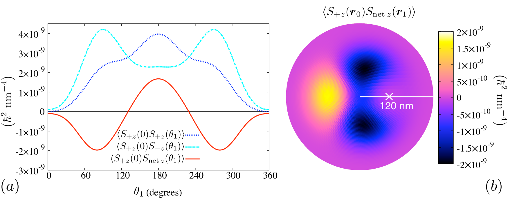
Figure 9: (Color online.) Two-point spin correlations in the four-particle ground state manifold. (a) Trace is along the ring of maximum single-particle density $r_{\text{max}}$ = 48 nm, with respect to a spin-up particle located at $\boldsymbol{{r}}_{0}=(r_{\text{max}},0^{\circ})$. (b) Net spin in the QD, given a spin-up particle at $\boldsymbol{{r}}_{0}=(r_{\text{max}},0^{\circ})$.

Figure 9(b) shows the evident antiferromagnetic tendency in the four-particle ground-state manifold. However, as shown in Fig. 9(a), in this small system, the spins are neither fully localized nor fully polarized in the quantum dot.

In the four-particle ground-state manifold, the net spin density from the two-point calculation shows canting along the ring $r_{\text{max}}$ as a function of $\theta_{1}$ similar to that in the three-particle ground-state manifold. The canting angle becomes antiparallel ($\alpha=180^{\circ}$) relative to the spin-up particle at $\boldsymbol{{r}}_{0}=(r_{\text{max}},\,0)$ as $\theta_{1}$ approaches zero, passing through the $x$-$y$ plane when the net spin density from the two-point function is zero along the ring $r_{\text{max}}$ (near $\theta_{1}=130^{\circ}$ and $\theta_{1}=230^{\circ}$), and has a positive projection on the $z$-axis at $\theta_{1}=180^{\circ}$, where the two-point function shows the net spin density to be predominantly spin-up. The canting angle along $r_{\text{max}}$ is consistent with the antiferromagnetic ordering suggested by the two-point correlation calculations. The result is shown in Fig. 10.

Figure 10: (Color online.) Canting angle $\alpha$ as a function of $\theta_{1}$ along the ring of maximum single-particle density $r_{\text{max}}$ = 48 nm in the four-particle ground state manifold. The net spin density from the two-point calculation along the same ring $r_{\text{max}}$ is shown for reference.

To investigate possible chiral textures, we examine three-point spin correlations in the four-particle ground-state manifold with respect to one particle spin-up along the $x$-axis at $\boldsymbol{{r}}_{0}$, and a second particle spin-up along the $y$-axis at $\boldsymbol{{r}}_{1}\equiv(r_{\text{max}},\theta_{1})$. Figure 11(a) shows the net $x$ spin distribution and Fig. 11(b) shows the net $y$ spin distribution in the system at every angular position $\theta_{2}$ as a function of $\theta_{1}$. (The net $z$ correlations are negligible and not shown.)

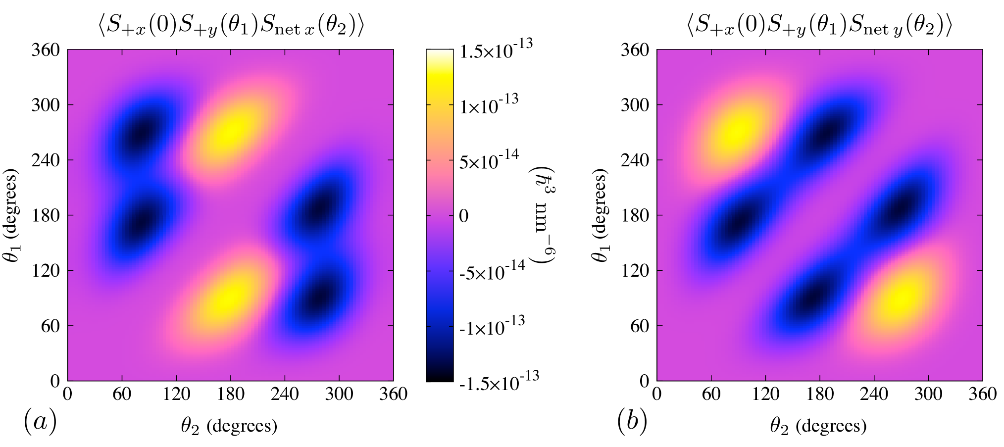
Figure 11: (Color online.) Three-point spin correlations along the ring of maximum single-particle density $r_{\text{max}}$ = 48 nm for the four-particle ground state. Specifically, the net $S_{x}$ (a) and net $S_{y}$ (b) are determined with respect to a particle of spin-up projection along the $x$-axis at $\boldsymbol{{r}}_{0}=(r_{\text{max}},\,0)$ and a particle of spin-up projection along the $y$-axis at $\boldsymbol{{r}}_{1}=(r_{\text{max}},\theta_{1})$.

As $\theta_{1}$ approaches 90^∘, two peaks (the two remaining particles) emerge in the net $x$ and $y$ spin distributions at $\theta_{2}=180^{\circ}$ and $\theta_{2}=270^{\circ}$. As $\theta_{1}$ approaches 180^∘, two different peaks arise at $\theta_{2}=90^{\circ}$ and $\theta_{2}=270^{\circ}$. There is a third region, at $\theta_{1}=270^{\circ}$ of large correlation that mirrors that at $\theta_{1}=90^{\circ}$. Note the inversion symmetry through the point $(\theta_{1},\theta_{2})=(180^{\circ},180^{\circ})$. Figure 12 focuses on the two regions of large correlation, when $\theta_{1}=90^{\circ}$ and 180^∘, showing the net $x$, $y$, and $z$ spin distributions as a function of $\theta_{2}$.

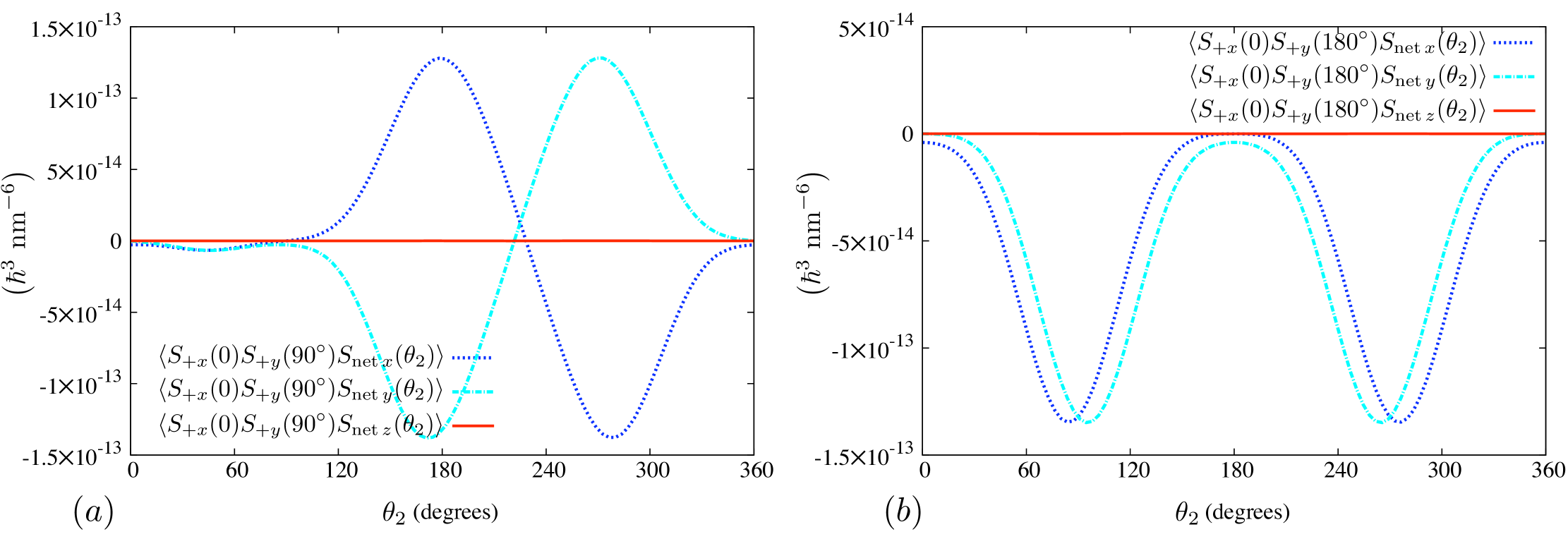
Figure 12: (Color online.) Three-point spin correlations along the ring of maximum single-particle density $r_{\text{max}}=48$ nm in the four-particle ground-state manifold with respect to a particle that is spin-up along the $x$-axis at $\boldsymbol{{r}}_{0}=(r_{\text{max}},\,0)$ and a particle that is spin-up along the $y$-axis at $\boldsymbol{{r}}_{1}=(r_{\text{max}},90^{\circ})$ (a) and $\boldsymbol{{r}}_{1}=(r_{\text{max}},180^{\circ})$ (b).

From these plots we conclude that chiral spin structures exist in the ground-state manifold of the interacting four-particle system, but the structures cannot be readily characterized by a definite winding about any axis.

We now go on to consider the lowest-energy excitation above this ground-state manifold, where we $do$ uncover winding textures.

V.2 First Excited State

The first excited state in the four-particle system is non-degenerate with quantum numbers $L_{z}=0$, $S=0$. It too has a circularly symmetric single-particle density distribution about the origin, with a peak at $r_{\text{max}}\equiv 48$ nm.

Figure 13 shows the two-point spin correlations throughout the plane of the dot with respect to a spin-up particle at $\boldsymbol{{r}}_{0}\equiv(r_{\text{max}},\,0)$. The distribution of the spin-up and spin-down densities are shown.

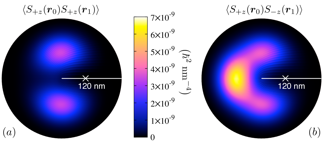
Figure 13: (Color online.) Two-point spin correlations in the first excited state of the four-particle system with respect to a spin-up particle at $\boldsymbol{{r}}_{0}=(48~{}\text{nm},\,0)$ (white cross). Shown are the spin-up (a) and spin-down (b) distributions.

The spin-up density shown in Fig. 13(a) contains two peaks at $\theta_{1}=90^{\circ}$ and $\theta_{1}=270^{\circ}$, both along the ring $r_{\text{max}}$. The probability drops to approximately one tenth of its magnitude between the peaks, at $\theta_{1}=180^{\circ}$. The spin density goes to zero as $\boldsymbol{{r}}_{1}$ approaches $\boldsymbol{{r}}_{0}$, giving evidence for a Pauli vortex at $\boldsymbol{{r}}_{0}$. The spin-down density shown in Fig. 13(b) has three peaks, the largest at $\theta_{1}=180^{\circ}$, and two smaller ones of equal magnitude at $\theta_{1}=90^{\circ}$ and $\theta_{1}=270^{\circ}$. In contrast to the ground state (see Fig. 8), this manifold does not exhibit antiferromagnetic order.

The two smaller peaks in the spin-down distribution are approximately half the magnitude of the large peak and approximately equal to the magnitude of the two peaks in the spin-up distribution. The net $S_{z}$ distribution at $\theta_{1}=90^{\circ}$ and $\theta_{1}=270^{\circ}$ is therefore approximately zero, indicating an in-plane orientation. This is further evident in the trace along the ring $r_{\text{max}}$ shown in Fig. 14(a), and the net spin distribution shown in Fig. 14(b).

Figure 14: (Color online.) (a) Trace of the two-point spin distribution along the ring $r_{\text{max}}=48$ nm with respect to a spin-up particle at $\boldsymbol{{r}}_{0}=(48~{}\text{nm},\,0)$ in the four-particle first excited state. (b) Net two-point distribution of $S_{z}$ throughout the QD for the same state.

The single peak at $\theta_{1}=180^{\circ}$ is composed primarily of a single spin-species. These results are consistent with two-point spin correlations in Ref. Ghosal et al., 2007. Of note here is that, in the transition from spin-up at $\theta_{1}=0^{\circ}$ to spin-down at $\theta_{1}=180^{\circ}$, the spin lies almost completely in the plane of the QD. Calculation of the canting angle along the ring $r_{\text{max}}$ as a function of $\theta_{1}$ is plotted in Fig. 15.

Figure 15: (Color online.) Canting angle $\alpha$ as a function of $\theta_{1}$ along the ring $r_{\text{max}}=48$ nm in the four-particle first excited state. The net spin density from the two-point calculation along the same ring $r_{\text{max}}$ is shown for reference.

In this case there are two locations where the net spin has the greatest canting. Relative to the spin-up particle at $\boldsymbol{{r}}_{0}=(r_{\text{max}},\,0)$, as $\theta_{1}$ approaches $\theta_{0}$ = 0 and also as $\theta_{1}$ approaches 180^∘, the canting angle approaches 180^∘. In the regions along $r_{\text{max}}$ where the net spin distribution is almost zero, the canting angle approaches 90^∘, showing that the net spin exists in the x-y plane. However, the two-point correlation function is incapable of determining the orientation of the spin within the plane. We therefore turn to the three-point correlation function in order to determine the orientation of the in-plane spin component as it transitions between spin-up and spin-down.

We calculate three-point spin correlations along the ring $r_{\text{max}}$ with respect to a spin-up particle along the $x$-axis at $\boldsymbol{{r}}_{0}=(r_{\text{max}},\,0)$, and a spin-up particle along the $y$-axis at $\boldsymbol{{r}}_{1}=(r_{\text{max}},\theta_{1})$. The net $x$ and net $y$ spin distributions are shown in Fig. 16 as a function of $\theta_{1}$ and $\theta_{2}$.

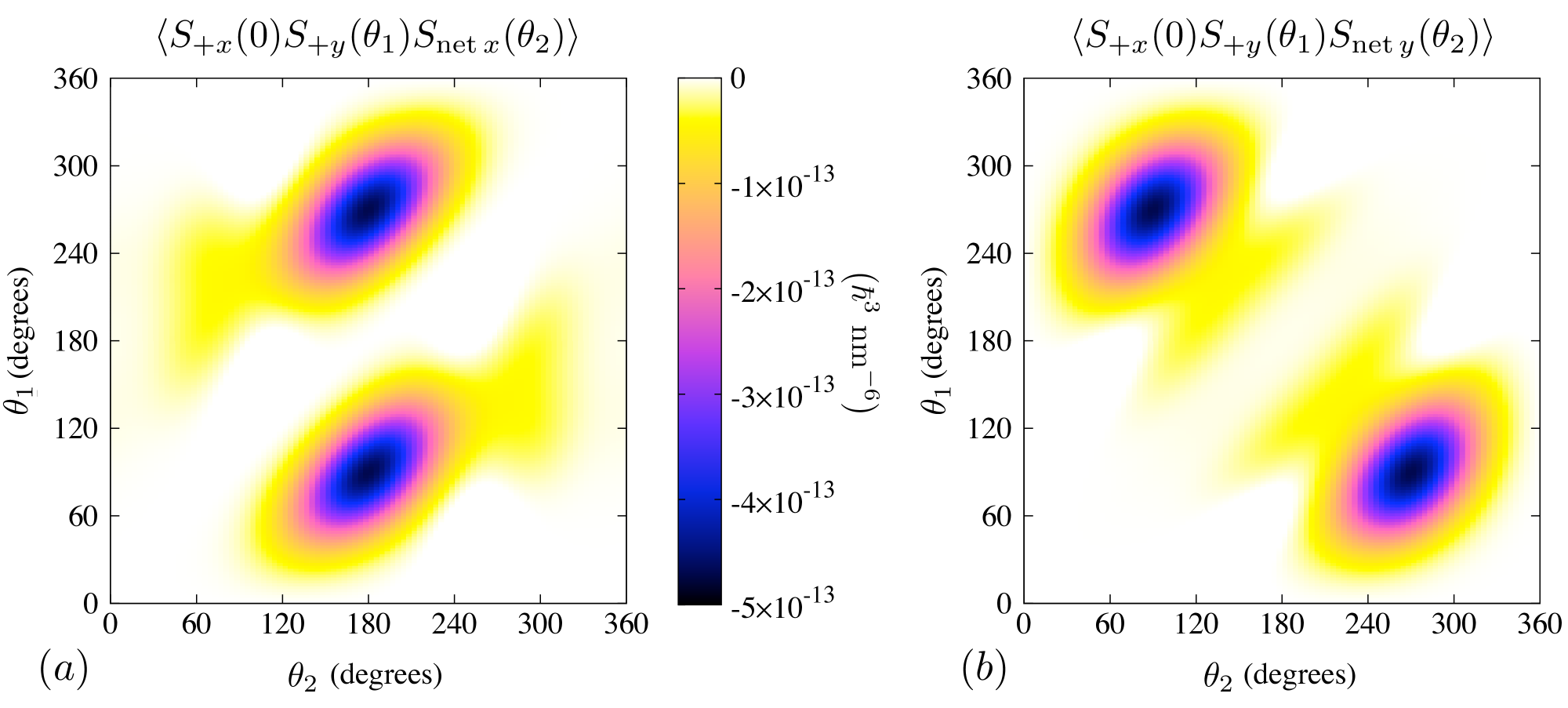
Figure 16: (Color online.) Three-point correlations along the ring $r_{\text{max}}=48$ nm in the four-particle first excited state with respect to a spin-up particle along the $x$-axis at $\boldsymbol{{r}}_{0}=(r_{\text{max}},\,0)$ and a spin-up particle along the $y$-axis at $\boldsymbol{{r}}_{1}=(r_{\text{max}},\,\theta_{1})$. Shown are the spin distributions along $\boldsymbol{{r}}_{2}=(r_{\text{max}},\,\theta_{2})$ for the net spin along the $x$-axis (a) and along the $y$-axis (b).

These distributions reveal strong correlations at $\theta_{1}=90^{\circ}$ and $\theta_{1}=270^{\circ}$, consistent with the previous two-point correlation. Note the inversion symmetry about the point $(\theta_{1},\theta_{2})=(180^{\circ},180^{\circ})$. The plots further show that for $\theta_{1}=90^{\circ}$, ($270^{\circ}$), the net spin is predominantly spin-down along $x$ at $\theta_{2}=180^{\circ}$, and predominantly spin-down along $y$ at $\theta_{2}=270^{\circ}$ ($90^{\circ}$). Focusing attention to the case of $\theta_{1}=90^{\circ}$, we plot in Fig. 17(a) the spin distribution along the ring $r_{\text{max}}$ given a spin-up particle along $x$ at $\theta_{0}=0^{\circ}$ and a spin-up particle along $y$ at $\theta_{1}=90^{\circ}$. Figure 17(b) shows the effect of this correlation on the net spin distribution throughout the plane of the quantum dot.

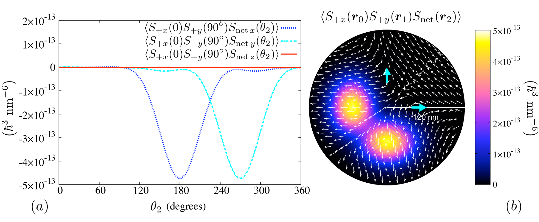
Figure 17: (Color online.) (a) Trace along the ring $r_{\text{max}}$, revealing the net spin distributions in the four-particle first excited state given a spin-up particle along $x$ at $\boldsymbol{{r}}_{0}=(r_{\text{max}},\,0)$ and a spin-up particle along $y$ at $\boldsymbol{{r}}_{1}=(r_{\text{max}},\,90^{\circ})$. (b) The corresponding net spin distribution in the plane of the QD. The vector field depicts the orientation and the color depicts the magnitude. The locations $\boldsymbol{{r}}_{0}$ and $\boldsymbol{{r}}_{1}$ are indicated by the blue arrows.

These results for the net $x$ and $y$ spin distributions are consistent with the $z$ distributions calculated by the two-point correlations (see Fig. 14). Those two-point correlations revealed a single peak at $180^{\circ}$ indicating a spin anti-aligned to the one at $\theta_{0}=0$ along the ring $r_{\text{max}}$. The three-point function with respect to a spin-up particle along $x$ at $\boldsymbol{{r}}_{0}=(r_{\text{max}},\,0)$ and a spin-up particle along $y$ at $\boldsymbol{{r}}_{1}=(r_{\text{max}},\,90^{\circ})$ yields a net spin polarized along the negative $x$-axis at $\theta=180^{\circ}$, and a net spin polarized along the negative $y$-axis at $\theta=270^{\circ}$, on the ring $r_{\text{max}}$. This is evidence of a winding along the ring $r_{\text{max}}$. From the symmetry of our correlation operators, Eq. (13a), we can deduce that there are in fact four orthogonal windings that wind about the origin in this manner; two which begin with a particle spin-up along the $x$-axis at $\boldsymbol{{r}}_{0}=(r_{\text{max}},\,0)$ and then differ in the direction of their spin polarization along the $y$-axis at $\boldsymbol{{r}}_{1}=(r_{\text{max}},\,90^{\circ})$ (i.e. in the chirality of the rotation), and two which begin with a particle spin-down along the $x$-axis at $\boldsymbol{{r}}_{0}=(r_{\text{max}},\,0)$, and again differ in their chirality along the ring $r_{\text{max}}$. Thus, we can characterize the first excited state of the four-particle droplet as a superposition of four different windings, differing by their chirality (clockwise and counter clockwise), and by a topological charge ($\pm 1$). (See Ref. Loss and Braun, 1996 for a thorough semiclassical description).

VI Summary

We have computed spin correlations in the two lowest-lying states of three-particle and four-particle circular two-dimensional QDs to resolve spin textures that exist in the system in the presence of strong, long-range Coulomb repulsion at zero magnetic field. Our findings are summarized in Table 1.

Table 1: Summary of textures uncovered in the respective degenerate manifolds.

Manifold	Single Particle Densities	2 Point	3 Point	Canting
3-particle ground state	$r_{max}=39$ nm	triangular lattice	splayed	131∘∗
3-particle first excited state	$r_{max}=41$ nm	triangular lattice	splayed	53∘
4-particle ground state	$r_{max}=48$ nm	antiferromagnetic order	no winding	varies
4-particle excited state	$r_{max}=48$ nm	in-plane configuration	in-plane winding	varies

^∗(at peaks)

From the one-point correlation, we determine the annular regions of maximum spin-density in the QD. As expected, the radial distance of this region from the origin depends on the number of confined particles, and on the strength of the Coulomb repulsion.

We further compute two-point spin correlation functions to determine the correlations in the spin field along a given direction. Each resulting spin distribution is symmetric through the diameter of the QD on which one particle is located. The details of the spin configurations are dependent on the unique quantum characteristics of the state, particularly the spin and orbital angular momentum quantum numbers. The two-point correlation calculations for each state suggest the presence of a Pauli vortex at the position of the fixed particle. In addition, these results reveal an incipient Wigner phase in the states examined above.

To uncover chiral textures, the three-point spin correlations are calculated. We plot the spin density with respect to two particles with mutually perpendicular spins. The three-particle states we have investigated exhibit splayed textures. The four-particle ground state exhibits an antiferromagnetic texture, and the first excited state exhibits winding textures. Here, the results indicate that, given a particle with spin at a point in the dot, the spin field rotates through a plane perpendicular to the original spin orientation with a full $2\pi$ winding as one moves along a closed trajectory about the origin. Importantly, given the finite size of the system and the full O(3) spin symmetry present, these winding textures are only quasi-topological in character. The rotational spin symmetry, in particular, allows the spins to continually deform into the trivial texture (or, rather, to the ground-state texture). In a larger, semiclassical system with at least uniaxial anisotropy, the analogous textures will have topological character. In fact, in 2DEGs and bulk systems, skyrmions and other spin textures have been shown to exist.Kumada et al. (2006); Khandelwal et al. (2001); Gervais et al. (2005); Hsieh et al. (2009); Mühlbauer et al. (2009)

In the present small but fully quantum system, incipient topological structures may manifest themselves if a coupling were introduced between the spin field and the spatial orientation of the quantum dot itself, analogous to the anisotropies typically found in much larger magnetic systems. This could come about through spin-orbit coupling. There is evidence that such a coupling may break the degeneracy between the spin-winding states.Stevenson and Kyriakidis (2010) Together with the strong Coulomb repulsion present in these small quantum systems, the chiral structures that emerge should exhibit longer lifetimes and lower decoherence rates than their more conventional counterparts.

Improvements in the lifetime of these states could be determined, for example, by comparing the relaxation rates of the states at and away from their degeneracy point by use of single-shot measurements.Hanson et al. (2005); Barthel et al. (2009) Experimental methods exist for differentiating between fully polarized spin states and correlated spin texture states in the ground state of a QD by measuring the excitation spectra of the QD as a function of magnetic field.Ciorga et al. (2003); Sachrajda et al. (2004); Nishi et al. (2006) These methods can be used to determine when a spin texture state is present in the system. The issues of spin-orbit coupling and state lifetimes will be investigated in future work.

Appendix Derivation of Product Spin Operators

In this appendix we discuss the general properties of the product-operators used in our above analysis, as well as the details associated with the derivation of each product-operator.

A.1 One-Body Spin Operators

A general one-body operator is expressed in canonical second-quantized form as

$$\hat{U}=\sum_{\alpha\,\beta}U_{\alpha\beta}\,\hat{c}_{\alpha}^{\dagger}\,\hat{c}^{\phantom{\dagger}}_{\beta},$$ (16)

where $U_{\alpha\beta}=\left({\alpha}\right|\hat{U}\left|{\beta}\right)$ is a matrix element of the operator,Negele and Orland (1988) and $\hat{c}_{\alpha}^{\dagger}$ and $\hat{c}^{\phantom{\dagger}}_{\alpha}$ are second-quantized Fermi operators, respectively creating and destroying a particle in state $|\alpha\rangle$.

For a system of spin-1/2 fermions, the operator for the spin density at position $\boldsymbol{{r}}$ is given by ($\hbar=1$)

$$\widehat{\boldsymbol{{S}}}(\boldsymbol{{r}})=\frac{1}{2}\sum_{ss^{\prime}}\hat{\psi}_{s}^{\dagger}(\boldsymbol{{r}})\boldsymbol{{\widehat{\sigma}}}^{ss^{\prime}}\hat{\psi}_{s^{\prime}}(\boldsymbol{{r}}),$$ (17)

where $\boldsymbol{{\widehat{\sigma}}}=(\hat{\sigma}_{x},\hat{\sigma}_{y},\hat{\sigma}_{z})$ are the Pauli spin matrices and $\hat{\psi}_{s}^{\dagger}(\boldsymbol{{r}})$ and $\hat{\psi}_{s}(\boldsymbol{{r}})$ are the field operators.

Equation (17) yields the net spin density at point $\boldsymbol{{r}}$. We are additionally interested in distinguishing the spin-up and spin-down densities along each coordinate-axis. We define a general set of spin operators $\hat{S}_{\pm\alpha}(\boldsymbol{{r}})$ that separately determines the spin-up and spin-down densities along $\alpha=x,y,z$ at position $\boldsymbol{{r}}$. In the $S_{z}$ basis, the operator for the $\pm x$ spin density, for example, is given by

$$\hat{S}_{\pm x}(\boldsymbol{{r}})=\frac{1}{4}\left[\left(\hat{\psi}_{\uparrow}^{\dagger}(\boldsymbol{{r}})\hat{\psi}_{\uparrow}^{\phantom{\dagger}}(\boldsymbol{{r}})+\hat{\psi}_{\downarrow}^{\dagger}(\boldsymbol{{r}})\hat{\psi}_{\downarrow}^{\phantom{\dagger}}(\boldsymbol{{r}})\right)\right.\\ \pm\left.\left(\hat{\psi}_{\uparrow}^{\dagger}(\boldsymbol{{r}})\hat{\psi}_{\downarrow}^{\phantom{\dagger}}(\boldsymbol{{r}})+\hat{\psi}_{\downarrow}^{\dagger}(\boldsymbol{{r}})\hat{\psi}_{\uparrow}^{\phantom{\dagger}}(\boldsymbol{{r}})\right)\right].$$ (18)

This operator can be derived from the field operators, $\hat{\psi}_{\pm x}^{\dagger}(\boldsymbol{{r}})=[\hat{\psi}_{\uparrow}^{\dagger}(\boldsymbol{{r}})\pm\hat{\psi}_{\downarrow}^{\dagger}(\boldsymbol{{r}})]/\sqrt{2}$, and $\hat{S}_{\pm x}(\boldsymbol{{r}})=\hat{\psi}_{\pm x}^{\dagger}(\boldsymbol{{r}})\hat{\psi}_{\pm x}(\boldsymbol{{r}})/2$. Similarly, the operators along the other two orthogonal directions are

$$\hat{S}_{\pm y}(\boldsymbol{{r}})=\frac{1}{4}\left[\left(\hat{\psi}_{\uparrow}^{\dagger}(\boldsymbol{{r}})\hat{\psi}_{\uparrow}^{\phantom{\dagger}}(\boldsymbol{{r}})+\hat{\psi}_{\downarrow}^{\dagger}(\boldsymbol{{r}})\hat{\psi}_{\downarrow}^{\phantom{\dagger}}(\boldsymbol{{r}})\right)\right.\\ \pm\left.i\left(\hat{\psi}_{\downarrow}^{\dagger}(\boldsymbol{{r}})\hat{\psi}_{\uparrow}^{\phantom{\dagger}}(\boldsymbol{{r}})-\hat{\psi}_{\uparrow}^{\dagger}(\boldsymbol{{r}})\hat{\psi}_{\downarrow}^{\phantom{\dagger}}(\boldsymbol{{r}})\right)\right],$$ (19)

and

$$\hat{S}_{+z}(\boldsymbol{{r}})=\frac{1}{2}\hat{\psi}_{\uparrow}^{\dagger}(\boldsymbol{{r}})\hat{\psi}_{\uparrow}^{\phantom{\dagger}}(\boldsymbol{{r}}),\quad\hat{S}_{-z}(\boldsymbol{{r}})=\frac{1}{2}\hat{\psi}_{\downarrow}^{\dagger}(\boldsymbol{{r}})\hat{\psi}_{\downarrow}^{\phantom{\dagger}}(\boldsymbol{{r}}).$$ (20)

By defining the net spin along an axis to be the difference between the spin-up and the spin-down density along that same axis ($\hat{S}_{x}(\boldsymbol{{r}})=\hat{S}_{+x}(\boldsymbol{{r}})-\hat{S}_{-x}(\boldsymbol{{r}})$, etc.), we obtain the components of Eq. (17). Upon integrating these net spin components over all space, we recover the usual expressions $\hat{S}_{x}=(\hat{S}_{+}+\hat{S}_{-})/2$, $\hat{S}_{y}=(\hat{S}_{+}-\hat{S}_{-})/(2i)$, and $\hat{S}_{z}=(\hat{S}_{\uparrow}-\hat{S}_{\downarrow})/2$, where $\hat{S}_{+}$ and $\hat{S}_{-}$ are $S_{z}$ raising and lowering operators, respectively.

The operators in Eqs. (18, 19) each contain terms which flip spins. But since the Hamiltonian, Eq. (1), conserves spin, and since we include spin quantum numbers to classify our states, these terms give zero contribution to Eq. (5a) for one-body spin operators. As a consequence of spin conservation we have for any degenerate manifold at zero magnetic field, $\langle S_{x}(\boldsymbol{{r}})\rangle=\langle S_{y}(\boldsymbol{{r}})\rangle=\langle S_{z}(\boldsymbol{{r}})\rangle=0$. Along the quantization ($z$) axis, we can distinguish between the spin-up and the spin-down density at position $\boldsymbol{{r}}$, but we cannot distinguish between the spin-up and spin-down density along the two orthogonal directions: Formally, $\langle S_{+x}(\boldsymbol{{r}})\rangle=\langle S_{-x}(\boldsymbol{{r}})\rangle$, and similarly for the $y$ direction. Consequently, it suffices to calculate only the one-point correlations of $\hat{S}_{\pm z}(\boldsymbol{{r}})$, as in Eq. (6).

A.2 Two-Body Spin Operators

To investigate correlations along a particular axis, the two-point correlations functions are required. On physical grounds, we require that operators be symmetric in their indexes.Negele and Orland (1988) For one-body operators, we require that $U_{\alpha\beta}=U_{\beta\alpha}$. For a two-body operator, we similarly require that $V_{\alpha\beta\gamma\delta}=V_{\beta\alpha\delta\gamma}$. In general, a product of $N$ one-body operators is not an $N$-body operator. Let $\hat{U}$ and $\hat{V}$ each be a one-body operator. Their product can be written as

$$\hat{U}\hat{V}=\sum_{ij}(UV)_{ij}\,\hat{c}_{i}^{\dagger}\hat{c}_{j}^{\phantom{\dagger}}\\ +\frac{1}{2}\sum_{ijkl}\left(U_{ik}V_{jl}+U_{jl}V_{ik}\right)\hat{c}_{i}^{\dagger}\hat{c}_{j}^{\dagger}\hat{c}_{l}^{\phantom{\dagger}}\hat{c}_{k}^{\phantom{\dagger}},$$ (21)

where $(UV)_{ij}\equiv\left({i}\right|\hat{U}\hat{V}\left|{j}\right)$, $U_{ik}V_{jl}\equiv\left({i}\right|\hat{U}\left|{k}\right)\left({j}\right|\hat{V}\left|{l}\right)$. The product of two one-body operators is in fact a sum of canonical one-body and two-body operators.

There is no preferred axis along which to calculate our two-point correlations because the net spin in each degenerate manifold is zero, but one may exploit the symmetry; for example, the correlation between a spin-up particle and the remaining spin-up distribution is identical to the correlation between a spin-down particle and the remaining spin-down distribution. In general, the correlations between a particle with spin and the remaining particles of parallel spin will be the same for any orientation, as will the correlations between a particle with spin and the remaining particles of antiparallel-spin. Due to spin conservation, two-point correlations between particles with perpendicular spin do not provide additional correlation information and are therefore not considered.

The two-point correlations investigated above are $\langle S_{+z}(\boldsymbol{{r}}_{0})S_{+z}(\boldsymbol{{r}}_{1})\rangle$ and $\langle S_{+z}(\boldsymbol{{r}}_{0})S_{-z}(\boldsymbol{{r}}_{1})\rangle$ in Eq. (10). With the condition $\boldsymbol{{r}}_{0}\neq\boldsymbol{{r}}_{1}$ (while still allowing $\boldsymbol{{r}}_{0}\rightarrow\boldsymbol{{r}}_{1}$), the one-body term vanishes. As described in Sec. A.1, spin symmetry implies that all four of $\langle S_{+z}(\boldsymbol{{r}}_{0})S_{\pm x}(\boldsymbol{{r}}_{1})\rangle$ and $\langle S_{+z}(\boldsymbol{{r}}_{0})S_{\pm y}(\boldsymbol{{r}}_{1})\rangle$ are identical and equal to $\langle(S_{+z}(\boldsymbol{{r}}_{0})S_{+z}(\boldsymbol{{r}}_{1})+S_{+z}(\boldsymbol{{r}}_{0})S_{-z}(\boldsymbol{{r}}_{1}))\rangle/2$.

A.3 Three-Body Spin Operators

To probe for chiral textures, we compute the three-point correlation functions. These are a product of three one-body operators. In canonical form, the product of three one-body operators is the sum of a canonical one-body, two-body, and three-body operator,

$$\hat{U}\hat{V}\hat{W}=\sum_{i\,j}(UVW)_{ij}\,\hat{c}_{i}^{\dagger}\hat{c}_{j}+\frac{1}{2}\sum_{ijkl}\Bigl{(}(UV)_{ik}W_{jl}+U_{ik}(VW)_{kl}+(UW)_{ik}V_{kl}\\ \mbox{}+(UV)_{jl}W_{ik}+U_{jl}(VW)_{ik}+(UW)_{jl}V_{ik}\Bigr{)}\hat{c}_{i}^{\dagger}\hat{c}_{j}^{\dagger}\hat{c}_{l}^{\phantom{\dagger}}\hat{c}_{k}^{\phantom{\dagger}}\\ \mbox{}+\frac{1}{3!}\sum_{\begin{subarray}{c}ijk\\ lmn\end{subarray}}\Bigl{(}U_{il}V_{jm}W_{kn}+U_{il}V_{kn}W_{jm}+U_{jm}V_{il}W_{kn}\\ \mbox{}+U_{jm}V_{kn}W_{il}+U_{kn}V_{il}W_{jm}+U_{kn}V_{jm}W_{il}\Bigr{)}\hat{c}_{i}^{\dagger}\hat{c}_{j}^{\dagger}\hat{c}_{k}^{\dagger}\hat{c}^{\phantom{\dagger}}_{n}\hat{c}^{\phantom{\dagger}}_{m}\hat{c}^{\phantom{\dagger}}_{l},$$ (22)

where $(UVW)_{ij}=\left({i}\right|\hat{U}\hat{V}\hat{W}\left|{j}\right)$. Each of the matrix elements in Eq. (22) is symmetric under appropriate interchange of indexes; for a three-body matrix element $V_{ijklmn}$, for example, we require $V_{ijklmn}=V_{ikjlnm}$, and so on.

We express our three-point correlation operators in the symmetric form shown in Eq. (22). As in Sec A.2, spin symmetry implies that the one-body and two-body pieces of Eq. (22) vanish when $\boldsymbol{{r}}_{0}$, $\boldsymbol{{r}}_{1}$, and $\boldsymbol{{r}}_{2}$ are all different. Because our averages are taken with respect to spin-conserving states, we need only consider terms in the correlation function which themselves conserve spin. We can thus write the product operators as they are given in Eq. (13).

References

- Kouwenhoven et al. (2001) L. P. Kouwenhoven, D. G. Austing, and S. Tarucha, Rep. Prog. Phys. 64, 701 (2001).
- Bukowski and Simmons (2002) T. J. Bukowski and J. H. Simmons, Crit. Rev. Solid State 27, 119 (2002).
- Reimann and Manninen (2002) S. M. Reimann and M. Manninen, Rev. Mod. Phys. 74, 1283 (2002).
- Burkard (2006) G. Burkard, in Handbook of Theoretical and Computational Nanotechnology, edited by M. Rieth and W. Schommers (American Scientific Publishers, Stevenson Ranch, CA, 2006), Vol. 3.
- Engel et al. (2004) H.-A. Engel, L. P. Kouwenhoven, D. Loss, and C. M. Marcus, Quantum Inf. Process. 3, 115 (2004), eprint cond-mat/0409294.
- Krenner et al. (2005) H. J. Krenner, S. Stufler, M. Sabathil, E. C. Clark, P. Ester, M. Bichler, G. Abstreiter, J. J. Finley, and A. Zrenner, New J. Phys. 7, 184 (2005), eprint cond-mat/0505731.
- Taylor et al. (2005) J. M. Taylor, H.-A. Engel, W. Dür, A. Yacoby C. M. Marcus, P. Zoller, and M. D. Lukin, Nature Physics 1, 177 (2005).
- Foletti et al. (2009) S. Foletti, H. Bluhm, D. Mahalu, V. Umansky, and A. Yacoby, Nature Physics 5, 903 (2009).
- Laird et al. (2010) E. A. Laird, J. M. Taylor, D. P. DiVincenzo, C. M. Marcus, M. P. Hanson, and A. C. Gossard, Phys. Rev. B 82, 075403 (2010).
- Ghosal et al. (2007) A. Ghosal, A. D. Guclu, C. J. Umrigar, D. Ullmo, and H. U. Baranger, Phys. Rev. B 76, 085341 (2007).
- Ghosal et al. (2006) A. Ghosal, A. D. Guclu, C. J. Umrigar, D. Ullmo, and H. U. Baranger, Nature Physics 2, 336 (2006).
- Loss and DiVincenzo (1998) D. Loss and D. P. DiVincenzo, Phys. Rev. A 57, 120 (1998), eprint cond-mat/9701055.
- Burkard et al. (1999) G. Burkard, D. Loss, and D. P. DiVincenzo, Phys. Rev. B 59, 2070 (1999), eprint cond-mat/9808026.
- Hanson et al. (2007) R. Hanson, L. P. Kouwenhoven, J. R. Petta, S Tarucha, and L. M. K. Vandersypen, Rev. Mod. Phys. 79, 1217 (2007).
- Ramsay (2010) A. J. Ramsay, Semicond. Sci. Technol. 25, 103001 (2010).
- Averin and Goldman (2001) D. V. Averin and V. J. Goldman, Solid State Commun. 121, 25 (2001).
- Kitaev (2003) A. Y. Kitaev, Annals of Physics 303, 2 (2003).
- Das Sarma et al. (2005) S. Das Sarma, M. Freedman, and C. Nayak, Phys. Rev. Lett. 94, 166802 (2005).
- Bombin and Martin-Delgado (2007) H. Bombin and M. A. Martin-Delgado, Phys. Rev. Lett. 98, 160502 (2007), ISSN 0031-9007 (Print).
- DiVincenzo (2000) D. P. DiVincenzo, Fortschr. Phys. 48, 771 (2000).
- Duan et al. (2003) L.-M. Duan, E. Demler, and M. D. Lukin, Phys. Rev. Lett. 91, 090402 (2003), ISSN 0031-9007 (Print).
- Bertoni et al. (2005) A. Bertoni, M. Rontani, G. Goldoni, and E. Molinari, Phys. Rev. Lett. 95, 066806 (2005).
- Climente et al. (2006) J. I. Climente, A. Bertoni, M. Rontani, G. Goldoni, and E. Molinari, Phys. Rev. B 74, 125303 (2006).
- Climente et al. (2007) J. I. Climente, A. Bertoni, G. Goldoni, M. Rontani, and E. Molinari, Phys. Rev. B 76, 085305 (2007).
- Governale (2002) M. Governale, Phys. Rev. Lett. 89, 206802 (2002).
- Kumada et al. (2006) N. Kumada, K. Muraki, and Y. Hirayama, Science 313, 329 (2006).
- Nishi et al. (2006) Y. Nishi, P. A. Maksym, D. G. Austing, T. Hatano, L. P. Kouwenhoven, H. Aoki, and S. Tarucha, Phys. Rev. B 74, 033306 (2006).
- Ciorga et al. (2003) M. Ciorga, M. Korkusinski, M. Pioro-Ladriere, P. Zawadzki, P. Hawrylak, and A. S. Sachrajda, Phys. Stat. Sol. 238, 325 (2003).
- Sachrajda et al. (2004) A. S. Sachrajda, M. Korkusinski, P. Hawrylak, M. Ciorga, M. Pioro-Ladriere, and P. Zawadzki, J. Magn. Magn. Mater. 272, E1273 (2004).
- Khandelwal et al. (2001) P. Khandelwal, A. E. Dementyev, N. N. Kuzma, S. E. Barrett, L. N. Pfeiffer, and K. W. West, Phys. Rev. Lett. 86, 5353 (2001).
- Gervais et al. (2005) G. Gervais, H. L. Stormer, D. C. Tsui, P. L. Kuhns, W. G. Moulton, A. P. Reyes, L. N. Pfeiffer, K. W. Baldwin, and K. W. West, Phys. Rev. Lett. 94, 196803 (2005).
- Hsieh et al. (2009) D. Hsieh, Y. Xia, L. Wray, D. Qian, A. Pal, J. H. Dil, J. Osterwalder, F. Meier, G. Bihlmayer, C. L. Kane, Y. S. Hor, R. J. Cava, and M. Z. Hasan, Science 323, 919 (2009).
- Mühlbauer et al. (2009) S. Mühlbauer, B. Binz, F. Jonietz, C. Pfleiderer, A. Rosch, A. Neubauer, R. Georgii, and P. Böni, Science 323, 915 (2009).
- Saarikoski et al. (2004) H. Saarikoski, A. Harju, M. J. Puska, and R. M. Nieminen, Phys. Rev. Lett. 93, 116802 (2004).
- Tavernier, Anisimovas, and Peeters (2004) M. B. Tavernier, E. Anisimovas, and F. M. Peeters Phys. Rev. B 70, 155321 (2004).
- Saarikoski and Harju (2005) H. Saarikoski and A. Harju, Phys. Rev. Lett. 94, 246803 (2005).
- Yang et al. (2007) N. Yang, J. L. Zhu, Z. Dai, and Y. Wang (2007), eprint arXiv:cond-mat/0701766v1.
- Anisimovas, Tavernier, and Peeters (2008) E Anisimovas, M. B. Tavernier, and F. M. Peeters Phys. Rev. B 77, 045327 (2008).
- Yang et al. (2005) S.-R. Eric Yang, N. Y. Hwang, and S. Park, Phys. Rev. B 72, 165337 (2005).
- Petkovic and Milovanovic (2007) A. Petkovic and M. V. Milovanovic, Phys. Rev. Lett. 98, 066808 (2007).
- Milovanovic, Dobardzic, and Radovic (2009) M. V. Milovanovic, E. Dobardzic, and Z. Radovic, Phys. Rev. B 80, 125305 (2009).
- Moon et al. (1995) K. Moon, H. Mori, K. Yang, S. M. Girvin, A. H. MacDonald, L. Zheng, D. Yoshioka, and S. C. Zhang, Phys. Rev. B 51, 5138 (1995).
- Jacak et al. (1997) L. Jacak, P. Hawrylak, and A. Wójs, Quantum Dots (Springer, Berlin, 1997).
- (44) These orbital wave functions are well known. However, various errors in sign and factors exist in several published versions. The expression shown in Eq. (4) is correct both in terms of the energy eigenvalue, and, importantly, in terms of relations such as .
- Abramowitz and Stegun (1965) M. Abramowitz and I. A. Stegun, Handbook of mathematical functions: with formulas, graphs, and mathematical tables (Dover Publications, New York, 1965).
- Kyriakidis et al. (2002) J. Kyriakidis, M. Pioro-Ladriere, M. Ciorga, A. S. Sachrajda, and P. Hawrylak, Phys. Rev. B 66, 035320 (2002).
- Stevenson and Kyriakidis (2011) C. J. Stevenson and J. Kyriakidis, Can. J. Phys. 89, 213 (2011).
- Saarikoski et al. (2010) H. Saarikoski, S. M. Reimann, A. Harju, and M. Manninen, Rev. Mod. Phys. 82, 2785 (2010).
- Loss and Braun (1996) H.-B. Braun and D. Loss, Phys. Rev. B 53, 3237 (1996).
- Stevenson and Kyriakidis (2010) C. J. Stevenson and J. Kyriakidis (unpublished).
- Hanson et al. (2005) R. Hanson, L. H. Willems van Beveren, I. T. Vink, J. M. Elzerman, W. J. M. Naber, F. H. L. Koppens, L. P. Kouwenhoven, and L. M. K. Vandersypen, Phys. Rev. Lett. 94, 196802 (2005).
- Barthel et al. (2009) C. Barthel, D. J. Reilly, C. M. Marcus, M. P. Hanson, and A. C. Gossard, Phys. Rev. Lett. 103, 160503 (2009).
- Negele and Orland (1988) J. W. Negele and H. Orland, Quantum many-particle systems (Addison-Wesley, 1988).