The Betti numbers of the moduli space of stable sheaves of rank 3 on $\mathbb{P}^{2}$

Abstract.

This article computes the generating functions of the Betti numbers of the moduli space of stable sheaves of rank 3 on $\mathbb{P}^{2}$ and its blow-up $\mathbb{\tilde{P}}^{2}$. Wall-crossing is used to obtain the Betti numbers for $\mathbb{\tilde{P}}^{2}$. These can be derived equivalently using flow trees, which appear in the physics of BPS-states. The Betti numbers for $\mathbb{P}^{2}$ follow from those for $\mathbb{\tilde{P}}^{2}$ by the blow-up formula. The generating functions are expressed in terms of modular functions and indefinite theta functions.

1. Introduction

The Euler and Betti numbers of moduli spaces of stable sheaves on complex surfaces have received much attention in the past, both in mathematics and physics. Computation of the generating functions of these numbers is notoriously difficult; a generic result is only known for rank 1 sheaves [10]. Yoshioka [28, 29] has computed the generating functions of the Betti numbers for rank 2 sheaves on a ruled surface using wall-crossing. The generating functions for rank 2 sheaves on the projective plane $\mathbb{P}^{2}$ follow from these by the blow-up formula [28, 29]. Some qualitative differences appear for rank 3, in which case only three Poincaré polynomials are known [30]. Using a different approach, namely toric geometry, Refs. [17, 20, 27] have computed generating functions of the Euler numbers for sheaves of rank 2 and 3 on $\mathbb{P}^{2}$.

The connection between sheaves and $\mathcal{N}=4$ supersymmetric gauge theory relates the Euler number of the moduli space to the supersymmetric index (or BPS-invariant) [26]. Another consequence of this connection is that the $SL(2,\mathbb{Z})$ electric-magnetic duality group of gauge theory implies modular properties for the generating functions of the Euler numbers [26], which was verified among others for sheaves on $\mathbb{P}^{2}$ with rank 1 and 2 [10, 28]. Ref. [2] identified the modular properties for the Betti numbers, which correspond to refined BPS-invariants [7]. Although modularity has been proven useful for computations for rational surfaces [24, 31, 12], mathematical justifications of physical expectations, in particular a so-called holomorphic anomaly [26, 24], have been limited to rank $\leq$2 [10, 28, 31] since generating functions for $r>2$ were not known.

This motivated the present work, which computes the generating functions of the Betti numbers for stable sheaves with rank 3 on the rationally ruled surface $\mathbb{\tilde{P}}^{2}$ and on $\mathbb{P}^{2}$. Using the results from [22, 23, 2], the generating functions take a particularly compact form in terms of modular functions and indefinite theta functions. The latter are convergent sums over a subset of an indefinite lattice [11]. The lattice for rank 2 has signature $(1,1)$ and the corresponding functions are well-studied in the literature [11, 33]. Interestingly, the lattice for rank 3 has signature $(2,2)$ and the corresponding function is of a novel form. A detailed discussion of the modular properties of this function will appear in a future article [3].

The computations in this article rely on wall-crossing and the blow-up formula, analogously to the computations by Yoshioka for rank 2, and can be extended to rank $>3$ if desired. To arrive at the generating functions, the (semi-primitive) wall-crossing formula of [5, 7] is applied to determine the change of the Betti numbers across a wall of marginal stability. This wall-crossing formula is derived in physics both for field theory [9] and for supersymmetric black holes in supergravity [5, 1], which correspond to D$p$-branes (or sheaves) supported on $p$-cycles of a Calabi-Yau threefold. The validity of the wall-crossing formula for this article can be motivated by viewing the surface as a (rigid) divisor of a Calabi-Yau threefold, and it is further confirmed by agreement of the generating functions with older results in the mathematical literature [30, 20, 27]. It is well-known that this wall-crossing formula is equivalent with the mathematical wall-crossing formulas derived for Donaldson-Thomas invariants [16, 18]. In fact, also mathematical arguments exist that these formulas are applicable for invariants of moduli spaces of sheaves on $\tilde{\mathbb{P}}^{2}$ since $K^{-1}_{\tilde{\mathbb{P}}^{2}}$ is numerically effective [15, 19].

Wall-crossing for sheaves (or D4-branes) supported on divisors in Calabi-Yau threefolds [22] is another motivation for this paper. Considering the sheaves on surfaces without the embedding into a Calabi-Yau simplifies the system and in this way helps to understand the Calabi-Yau case. On the other hand supergravity gives a useful complementary viewpoint, and suggests for example that the generating function for BPS-invariants can be computed using enumeration of so-called flow trees [4]. This approach was taken in [23], and the present article provides an illustration and confirmation of this technique. Subsection 2.3 gives a brief introduction to flow trees, however the discussion in this article is mostly phrased in terms of sheaves and characteristic classes, because the notion of a moduli space is most rigorously defined in this context.

The outline of the paper is as follows. Section 2 reviews the necessary properties of sheaves, including wall-crossing and blow-up formulas. Subsection 2.3 gives a brief introduction to flow trees. Section 3 computes the Euler numbers of the moduli spaces for rank 2 and 3, followed by the computation of the Betti numbers in Section 4. Appendix A lists various modular functions, which appear in the generating functions of the Euler and Betti numbers.

2. Sheaves

2.1. Sheaves and stability

The Chern character of a sheaf $F$ on a surface $S$ is given by ch$(F)=r(F)+c_{1}(F)+\frac{1}{2}c_{1}(F)^{2}-c_{2}(F)$ in terms of the rank $r(F)$ and its Chern classes $c_{1}(F)$ and $c_{2}(F)$. It is convenient to parametrize a sheaf by ch$(F)$ since it is additive: $\mathrm{ch}(F\oplus G)=\mathrm{ch}(F)+\mathrm{ch}(G)$. Define $\Gamma:=(r,\mathrm{ch}_{1},\mathrm{ch}_{2})$. Other frequently occuring quantities are the determinant $\Delta(F)=\frac{1}{r(F)}(c_{2}(F)-\frac{r(F)-1}{2r(F)}c_{1}(F)^{2})$, and $\mu(F)=c_{1}(F)/r(F)\in H^{2}(S,\mathbb{Q})$.

Let $0\subset F_{1}\subset F_{2}\subset\dots\subset F_{s}=F$ be a filtration of the sheaf $F$. The quotients are denoted by $E_{i}=F_{i}/F_{i-1}$ with $\Gamma_{i}=\Gamma(E_{i})$.

Lemma 2.1.

With the above notation, the discriminant $\Delta(F)$ is given by

$$\Delta(F)=\sum_{i=1}^{s}\frac{r(E_{i})}{r(F)}\Delta(E_{i})-\frac{1}{2r(F)}\sum_{i=2}^{s}\frac{r(F_{i-1})\,r(F_{i})}{r(E_{i})}\left(\mu(F_{i-1})-\mu(F_{i})\right)^{2}.$$

Proof.

Consider first the filtration for $s=2$: $0\subset F_{1}\subset F_{2}=F$, such that $\Gamma(F)=\Gamma(F_{1})+\Gamma(E_{2})$. Application of the definitions and some straightforward algebra lead to:

$$\Delta(F)=\frac{r(F_{1})}{r(F)}\Delta(F_{1})+\frac{r(E_{2})}{r(F)}\Delta(E_{2})-\frac{r(F_{1})r(E_{2})}{2r(F)^{2}}(\mu(F_{1})-\mu(E_{2}))^{2}.$$

Applying this equation iteratively on $F_{1}$ leads to the lemma. ∎

The notion of a moduli space for sheaves is only well defined after the introduction of a stability condition. To this end let $C(S)\in H^{2}(S,\mathbb{Z})$ be the ample cone of $S$.

Definition 2.2.

Given a choice $J\in C(S)$, a sheaf $F$ is called $\mu$-stable if for every subsheaf $F^{\prime}$, $\mu(F^{\prime})\cdot J<\mu(F)\cdot J$, and $\mu$-semi-stable if for every subsheaf $F^{\prime}$, $\mu(F^{\prime})\cdot J\leq\mu(F)\cdot J$. A wall of marginal stability $W$ is a (codimension 1) subspace of $C(S)$, such that $(\mu(F^{\prime})-\mu(F))\cdot J=0$, but $(\mu(F^{\prime})-\mu(F))\cdot J\neq 0$ away from $W$.

Let $S$ be a Kähler surface, whose intersection pairing on $H^{2}(S,\mathbb{Z})$ has signature $(1,b_{2}-1)$. Since at a wall, $(\mu_{2}-\mu_{1})\cdot J=0$ for $J$ ample, $(\mu_{2}-\mu_{1})^{2}<0$. Therefore, the set of filtrations for $F$, with $\Delta_{i}\geq 0$ is finite.

2.2. Invariants and wall-crossing

Ref. [26] shows that the BPS-invariant of $\mathcal{N}=4$ gauge theory on $S$ equals the Euler number (up to a sign) of a suitable compactification of the instanton moduli space, i.e. the Gieseker-Maruyama moduli space $\mathcal{M}_{J}(\Gamma)$ of semi-stable sheaves on $S$ (with respect to the ample class $J$). The topological classes $\Gamma$ of the sheaf are determined by the topological properties of the instanton. The complex dimension of $\mathcal{M}_{J}(\Gamma)$ is given by:

$$\dim_{\mathbb{C}}\mathcal{M}_{J}(\Gamma)=2r^{2}\Delta-r^{2}\chi(\mathcal{O}_{S})+1.$$

The BPS-invariant $\Omega(\Gamma;J)$ corresponds to the Euler number of $\mathcal{M}_{J}(\Gamma)$

$$\Omega(\Gamma;J)=(-1)^{\dim_{\mathbb{C}}\mathcal{M}_{J}(\Gamma)}\chi(\mathcal{M}_{J}(\Gamma)),$$

if the moduli space is smooth and compact. The mathematical rigorous definition of the BPS-invariant is more involved if these conditions are not satisfied [29]. The rational invariants [25, 16, 18]

(2.1) $$\bar{\Omega}(\Gamma;J)=\sum_{m|\Gamma}\frac{\Omega(\Gamma/m;J)}{m^{2}}$$

are also particularly useful for our purposes [23].

To state the changes $\Delta\Omega(\Gamma;J_{\mathcal{C}}\to J_{\mathcal{C}^{\prime}})$ across walls of marginal stability, we define the following quantities:

(2.2) $$\left<\Gamma_{1},\Gamma_{2}\right>=r_{1}r_{2}(\mu_{2}-\mu_{1})\cdot K_{S},\qquad\mathcal{I}(\Gamma_{1},\Gamma_{2};J)=r_{1}r_{2}(\mu_{2}-\mu_{1})\cdot J.$$

These definitions follow quite naturally from formulas in physics [6, 22, 23].

The change $\Delta\Omega(\Gamma_{1}+\Gamma_{2};J_{\mathcal{C}}\to J_{\mathcal{C}^{\prime}})$, for $\Gamma_{1}$ and $\Gamma_{2}$ primitive, is [30, 5]:

$$\Delta\Omega(\Gamma_{1}+\Gamma_{2};J_{\mathcal{C}}\to J_{\mathcal{C}^{\prime}}) = \textstyle{\frac{1}{2}}\left(\mathrm{sgn}(\mathcal{I}(\Gamma_{1},\Gamma_{2};J_{\mathcal{C}^{\prime}}))-\mathrm{sgn}(\mathcal{I}(\Gamma_{1},\Gamma_{2};J_{\mathcal{C}}))\right)$$

$$\times\,(-1)^{\left<\Gamma_{1},\Gamma_{2}\right>}\left<\Gamma_{1},\Gamma_{2}\right>\Omega(\Gamma_{1};J_{W_{\mathcal{C}}})\,\Omega(\Gamma_{2};J_{W_{\mathcal{C}}}),$$

with

$$\mathrm{sgn}(x)=\left\{\begin{array}[]{cl}1,&x>0,\\ 0,&x=0,\\ -1,&x<0.\end{array}\right.$$

The subscript ${W_{\mathcal{C}}}$ in $J_{W_{\mathcal{C}}}$ refers to a point in $\mathcal{C}$ which is sufficiently close to the wall $W$, such that no wall is crossed for the constituents between the wall and $J_{W_{\mathcal{C}}}$. The wall is independent of $c_{2}$, and therefore a sum over $c_{2}$ appears in the next section.

For the computation of the invariants for rank 3, one also needs the semi-primitive wall-crossing formula [5]:

$$\Delta\Omega(2\Gamma_{1}+\Gamma_{2};J_{\mathcal{C}}\to J_{\mathcal{C}^{\prime}}) = \textstyle{\frac{1}{2}}\left(\mathrm{sgn}(\mathcal{I}(\Gamma_{1},\Gamma_{2};J_{\mathcal{C}^{\prime}}))-\mathrm{sgn}(\mathcal{I}(\Gamma_{1},\Gamma_{2};J_{\mathcal{C}}))\right)$$

$$\times\left\{-2\left<\Gamma_{1},\Gamma_{2}\right>\Omega(2\Gamma_{1};J_{W_{\mathcal{C}}})\,\Omega(\Gamma_{2};J_{W_{\mathcal{C}}})\right.$$

$$\quad+(-1)^{\left<\Gamma_{1},\Gamma_{2}\right>}\left<\Gamma_{1},\Gamma_{2}\right>\Omega(\Gamma_{1};J_{W_{\mathcal{C}}})\,\Omega(\Gamma_{1}+\Gamma_{2};J_{W_{\mathcal{C}}})$$

$$\quad\left.+\textstyle{\frac{1}{2}}\left<\Gamma_{1},\Gamma_{2}\right>\Omega(\Gamma_{2};J_{W_{\mathcal{C}}})\,\Omega(\Gamma_{1};J_{W_{\mathcal{C}}})\,(\left<\Gamma_{1},\Gamma_{2}\right>\Omega(\Gamma_{1};J_{W_{\mathcal{C}}})-1)\right\}.$$

Define the generating function for $\bar{\Omega}(\Gamma;J)$:

(2.5) $$h_{r,c_{1}}(\tau;S,J):=\sum_{c_{2}}\bar{\Omega}(\Gamma;J)\,q^{r\Delta-\frac{r\chi(S)}{24}}.$$

Twisting a sheaf by a line bundle gives an isomorphism of moduli spaces, which implies $h_{r,c_{1}+\mathbf{k}}=h_{r,c_{1}}$ if $\mathbf{k}\in H_{2}(S,r\mathbb{Z})$. It is therefore sufficient to determine $h_{r,c_{1}}$ only for $c_{1}\mod r$. Explicit computation of $h_{r,c_{1}}(\tau;S,J)$ is typically complicated. A generic result exists just for $r=1$ [10]:

(2.6) $$h_{1,c_{1}}(\tau;S)=\frac{1}{\eta(\tau)^{\chi(S)}},$$

with $\eta(\tau)$ defined in Eq. (A). The dependence on $J$ could be omitted here, since the moduli space of rank 1 sheaves does not depend on a choice of ample class.

The next proposition gives the universal relation between generating functions for $S$ and its blow-up $\tilde{S}$. This appeared first for $r=2$ in [28, 26] and for general $r$ in [30]. Proofs are given in [21] for $r=2$, and [12] for general $r$.

Proposition 2.3.

Let $S$ be a smooth projective surface and $\phi:\tilde{S}\to S$ the blow-up at a non-singular point, with $C_{1}$ the exceptional divisor of $\phi$. Let $J\in C(S)$, $r$, and $c_{1}$ such that $\gcd(r,c_{1}\cdot J)=1$. The generating functions $h_{r,c_{1}}(\tau;S,J)$ and $h_{r,c_{1}}(\tau;\tilde{S},J)$ are then related by the “blow-up formula”:

$$h_{r,\phi^{*}c_{1}-kC_{1}}(\tau;\tilde{S},\phi^{*}J)=B_{r,k}(\tau)\,h_{r,c_{1}}(\tau;S,J),$$

with

$$B_{r,k}(\tau)=\frac{(-1)^{(r-1)k}}{\eta(\tau)^{r}}\sum_{\sum_{i=1}^{r}a_{i}=0\atop a_{i}\in\mathbb{Z}+\frac{k}{r}}q^{-\sum_{i<j}a_{i}a_{j}}.$$

The factor $(-1)^{(r-1)k}$ is a consequence of the relative sign between the BPS-invariant and the Euler number. The two relevant cases for this article are $r=2,3$:

(2.7) $$B_{2,k}(\tau)=(-1)^{k}\frac{\sum_{n\in\mathbb{Z}+k/2}q^{n^{2}}}{\eta(\tau)^{2}},\qquad B_{3,k}(\tau)=\frac{\sum_{m,n\in\mathbb{Z}+k/3}q^{m^{2}+n^{2}+mn}}{\eta(\tau)^{3}}.$$

2.3. Flow trees

This subsection gives a brief introduction to flow trees, since the computations in the next sections are inspired by it. More information can be found in Refs. [4, 5]. See Ref. [23] for a discussion which is more adapted to the present context.

Flow trees appear in the analysis of D-brane bound states. D-branes are equivalent to coherent sheaves in the “infinite volume limit”. A flow tree is an embedding of a rooted tree $T$ in $C(S)$ (or more generally, the moduli space), which satisfies a number of “stability” conditions. The tree can be parametrized by a nested list, e.g. $((\Gamma_{1},\Gamma_{2}),\Gamma_{3})$, and represents a decomposition of the total charge $\Gamma=\sum_{i}\Gamma_{i}$. The change of $J$ along the edges of the tree, is determined by the supergravity equations of motion. The endpoints of the flow tree represent “elementary” constituents which do not decay in $C(S)$, for example rank 1 sheaves. Generically, only in a special chamber in $C(S)$, the chamber with the attractor point, the total moduli space corresponds to the moduli space of these elementary constituents.

The existence of a tree as a flow tree is determined by “stability conditions” at its vertices. The class $J$ lies at a wall for the two merging trees if it is a trivalent vertex. For example, the stability of the subtree $(\Gamma_{1},\Gamma_{2})$ in $((\Gamma_{1},\Gamma_{2}),\Gamma_{3})$, is determined at a (specific) point of the wall for $\Gamma_{1}+\Gamma_{2}$ and $\Gamma_{3}$. If all conditions are satisfied the tree does exist as a flow tree. The attractor flow conjecture states that the “BPS Hilbert space” is partitioned by flow trees [1, 4]. This implies that the BPS-index can be computed in principle by enumerating flow trees, once the BPS-indices of the endpoints are known [5].

One of the advantages of flow trees is that they give an algorithmic procedure to test for the stability of a composite object at a given point in moduli space. A simplifying feature is that they do not distinguish between subobjects and quotients, in contrast to the stratification of the set of sheaves using (Harder-Narasimhan) filtrations.

Small changes are necessary to utilize flow trees in the present context, since the manifold is a surface instead of a 3-dimensional Calabi-Yau threefold. One difference is the choice of the boundary of $C(\mathbb{\tilde{P}}^{2})$ as reference point in the moduli space, instead of the attractor point. For $\mathbb{\tilde{P}}^{2}$ one does not need to solve for $J$ along the edges, not even for the flow trees with 3 centers, since a wall in $C(\mathbb{\tilde{P}}^{2})$ is only a single point (projectively). With these observations, it is not difficult to realize that the generating functions for the (refined) BPS-invariants in Sections 3 and 4 can be obtained either using wall-crossing or enumeration of flow trees.

3. Euler numbers

This section computes the generating function of Euler numbers of the moduli spaces of semi-stable sheaves of rank 2 and 3 on $\mathbb{\tilde{P}}^{2}$ and $\mathbb{P}^{2}$. First, some rudiments of ruled surfaces are reviewed.

3.1. Some properties of ruled surfaces

A ruled surface is a surface $\Sigma$ together with a surjective morphism $\pi:\Sigma\to C$ to a curve $C$, such that the fibre $\Sigma_{y}$ is isomorphic to $\mathbb{P}^{1}$ for every point $y\in C$. Let $f$ be the fibre of $\pi$, then $H_{2}(\Sigma,\mathbb{Z})=\mathbb{Z}C\oplus\mathbb{Z}f$, with intersection numbers $C^{2}=-e$, $f^{2}=0$ and $C\cdot f=1$. The canonical class is $K_{\Sigma}=-2C+(2g-2-e)f$. The holomorphic Euler characteristic $\chi(\mathcal{O}_{\Sigma})$ is for a ruled surface $1-g$. An ample divisor is parametrized as $J_{m,n}=m(C+ef)+nf$ with $m,n\geq 1$.

The blow-up $\phi:\mathbb{\tilde{P}}^{2}\to\mathbb{P}^{2}$ of the projective plane $\mathbb{P}^{2}$ at a point is equal to the rationally ruled surface with $(g,e)=(0,1)$. The exceptional divisor of $\phi$ is $C$, and the hyperplane $H$ of $\mathbb{P}^{2}$ equals $\phi^{*}(C+f)$. The remainder of this article restricts to the case $(g,e)=(0,1)$, although many results are easily generalized to generic $(g,e)$.

3.2. Rank 2

Our aim is to compute the generating function $h_{2,c_{1}}(\tau;\mathbb{\tilde{P}}^{2},J)$ defined by Eq. (2.5). To learn about the set of stable sheaves on $\mathbb{\tilde{P}}^{2}$ for $J\in C(S)$, it is useful to first consider the restriction of the sheaves on $\mathbb{\tilde{P}}^{2}$ to $f$. Namely the restriction $E_{|f}$ is stable if and only if $E$ is $\mu$-stable for $J=J_{0,1}$ and in the adjacent chamber [14]. However, since every bundle of rank $\geq 2$ on $\mathbb{P}^{1}$ is a sum of line bundles [13], there are no stable bundles with $r\geq 2$ on $\mathbb{P}^{1}$. Therefore $\Omega(\Gamma;J_{0,1})=0$ for $\Gamma=(r(F),-C-\alpha f,\mathrm{ch}_{2})$ with $r(F)\geq 2$ and $\alpha=0,1$. The computation for $c_{1}(E)=-\alpha f$ is more complicated, and is dealt with in the end of this subsection.

To determine $h_{2,-C-\alpha f}(\tau;J_{m,n})$, one can either change the polarization from $J_{0,1}$ to $J_{m,n}$ (see Figure 1) and keep track of $\Omega(\Gamma;J)$ across the walls, or enumerate the flow trees for $J_{m,n}$.

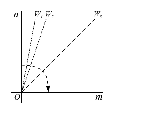
Figure 1. The ample cone of $\mathbb{\tilde{P}}^{2}$, together with the three walls for $\Gamma=(2,-C-f,2)$, namely for $(a,b)=(1,0)$, $(2,0)$, $(3,0)$.

The only possible filtrations are $0\subset F_{1}\subset F$, with $r_{i}=1$. Therefore the primitive wall-crossing formula (2.2) suffices, and the $\Omega(\Gamma_{i})$ do not depend on the moduli. In the following, $c_{1}(E_{2})$ is parametrised by $bC-af$. As is customary for flow trees, the constituents are treated symmetrically, such that $a,b$ run over $\mathbb{Z}$. Since $r_{1}=r_{2}$, this sum needs to be multiplied by $\textstyle{\frac{1}{2}}$. The walls are then at $\frac{m}{n}=\frac{2b+1}{2a-\alpha}$, with $m,n\geq 0$. See Figure 1 for the walls for $\Delta(F)=\frac{9}{4}$, $r(F)=2$.

The various quantities appearing in $h_{2,c_{1}}(\tau;J_{m,n})$ become in terms of $a$ and $b$:

$$\Delta(F) =\textstyle{\frac{1}{2}}\Delta_{1}+\textstyle{\frac{1}{2}}\Delta_{2}+\frac{1}{8}(2b+1)^{2}+\frac{1}{4}(2b+1)(2a-\alpha),$$

$$\left<\Gamma_{1},\Gamma_{2}\right> =-(2b+1)+2(2a-\alpha),$$

$$\mathcal{I}(\Gamma_{1},\Gamma_{2};J_{m,n}) =(2b+1)n-(2a-\alpha)m.$$

It is now straightforward to construct the generating function using (2.2):

$$h_{2,-C-\alpha f}(\tau;J_{m,n}) = -\frac{1}{2}\frac{1}{\eta(\tau)^{8}}\sum_{a,b\in\mathbb{Z}}\textstyle{\frac{1}{2}}(\,\mathrm{sgn}((2b+1)n-(2a-\alpha)m)-\mathrm{sgn}(2b+1)\,)$$

$$\times\,(-(2b+1)+2(2a-\alpha))\,q^{\frac{1}{4}(2b+1)^{2}+\frac{1}{2}(2b+1)(2a-\alpha)}.$$

The $-$-sign in front is due to $(-1)^{\left<\Gamma_{1},\Gamma_{2}\right>}$, the $\textstyle{\frac{1}{2}}$ appears because $r_{1}=r_{2}$, and $\eta(\tau)^{-8}$ arises from the sum over $\Delta_{i}$ and (2.6). Ref. [2] proved that for $J_{m,n}=J_{1,0}$, the generating functions are

(3.3) $$h_{2,-C-f}(\tau;J_{1,0})=3B_{2,0}(\tau)\mathfrak{h}_{1}(\tau)/\eta(\tau)^{6},$$

$$h_{2,-C}(\tau;J_{1,0})=3B_{2,1}(\tau)\mathfrak{h}_{0}(\tau)/\eta(\tau)^{6},$$

where $\mathfrak{h}_{i}(\tau)$ are generating functions of the class numbers (A.2). The half-integer coefficients for $c_{1}(F)=-C$ arise because $J_{1,0}$ is a wall for $F$. Application of Proposition 2.3 gives the known generating functions for $\mathbb{P}^{2}$ [26]. This gives incidentally also the correct result for $c_{1}(F)=0$, even though $\gcd(r(F),c_{1}(F)\cdot J)\neq 1$.

To compute $h_{3,-C-f}(\tau;J_{m,n})$, one needs explicit expressions for $h_{2,-\alpha f}(\tau;J_{m,n})$, $\alpha=0,1$. Fortunately, it is not necessary to deal with the singularities in the moduli space explicitly. One can either apply modular transformations or blow-down and blow-up again for $J_{m,n}=J_{1,0}$ and then apply the wall-crossing formula. One finds in both cases for $J_{1,0}$:

$$h_{2,-f}(\tau;J_{1,0})=-3B_{2,1}(\tau)\mathfrak{h}_{1}(\tau)/\eta(\tau)^{6},$$

$$h_{2,0}(\tau;J_{1,0})=-3B_{2,0}(\tau)\mathfrak{h}_{0}(\tau)/\eta(\tau)^{6}.$$

The Fourier coefficients $\bar{\Omega}(\Gamma;J_{1,0})$ of $h_{2,0}(\tau;J_{1,0})$ are not integers, since $\Gamma$ might be divisible by 2. One finds for the generating function of $\Omega(\Gamma;J_{1,0})$ using (2.1):

$$-3B_{2,0}(\tau)\mathfrak{h}_{0}(\tau)/\eta(\tau)^{6}-1/4\eta(2\tau)^{4}.$$

The wall-crossing formula provides now the generating functions for generic $J\in C(\mathbb{\tilde{P}}^{2})$:

(3.4) $$h_{2,\beta C-\alpha f}(\tau;J_{m,n})=h_{2,\beta C-\alpha f}(\tau;J_{1,0})+\Delta h_{2,\beta C-\alpha f}(\tau;J_{m,n}),$$

with

$$\Delta h_{2,\beta C-\alpha f}(\tau;J_{m,n})=$$

(3.5) $$\qquad(-)^{\beta}\frac{1}{2}\frac{1}{\eta(\tau)^{8}}\sum_{a,b\in\mathbb{Z}}\textstyle{\frac{1}{2}}(\,\mathrm{sgn}(-(2a-\alpha)\,)-\mathrm{sgn}((2b-\beta)n-(2a-\alpha)m)\,)$$

$$\qquad\times\,(-(2b-\beta)+2(2a-\alpha))\,q^{\frac{1}{4}(2b-\beta)^{2}+\frac{1}{2}(2b-\beta)(2a-\alpha)}.$$

3.3. Rank 3

Using the results of the previous subsection, the Euler numbers of the moduli space of stable sheaves with $\Gamma(F)=(3,-C-f,\mathrm{ch}_{2})$ can be computed. This computation has to deal with two additional complications:

• semi-primitive wall-crossing is possible for sheaves with $\Gamma(F)=2\Gamma_{1}+\Gamma_{2}$,

• the BPS-invariants of a constituent with $r=2$ do themselves depend on the moduli, and need to be determined sufficiently close to the appropriate wall.

Since no stable sheaves do exist for $c_{1}(F)=-C-f$, all sheaves are composed of 2 constituents with rank $r_{1}=1$ and $r_{2}=2$, or 3 constituents with rank $r_{i}=1$, $i=1,2,3$. Therefore the formulas of Ref. [23] for the enumeration of flow trees with 3 centers are applicable. There it was explained that the semi-primitive wall-crossing formula for $2\Gamma_{1}+\Gamma_{2}$ simplifies, if 1) the invariants are evaluated at a point on the wall $J_{W}$ instead of $J_{W_{\mathcal{C}}}$, and 2) it is written in terms of the rational invariant $\bar{\Omega}(\Gamma,J_{W})$. With these substitutions, one finds that Eq. (2.2) is equal to:

(3.6) $$\Delta\Omega(2\Gamma_{1}+\Gamma_{2};J_{\mathcal{C}}\to J_{\mathcal{C}^{\prime}}) = \textstyle{\frac{1}{2}}\left(\mathrm{sgn}(\mathcal{I}(\Gamma_{1},\Gamma_{2};J_{\mathcal{C}^{\prime}}))-\mathrm{sgn}(\mathcal{I}(\Gamma_{1},\Gamma_{2};J_{\mathcal{C}}))\right)\left<\Gamma_{1},\Gamma_{2}\right>$$

$$\times\left(-2\,\bar{\Omega}(2\Gamma_{1};J_{W})\,\Omega(\Gamma_{2})+(-1)^{\left<\Gamma_{1},\Gamma_{2}\right>}\,\Omega(\Gamma_{1})\,\Omega(\Gamma_{1}+\Gamma_{2};J_{W})\right).$$

One observes that the extra terms due to semi-primitive wall-crossing are naturally included into the terms for primitive wall-crossing.

The Euler numbers can now be obtained by simply implementing the formulas. Choose again $c_{1}(E_{2})=bC-af$. Then, the walls are at

$$\frac{m}{n}=\frac{3b+2}{3a-2},\qquad m,n\geq 0.$$

For the generating function follows:

$$h_{3,-C-f}(\tau;J_{m,n}) = \frac{1}{\eta(\tau)^{4}}\sum_{a,b\in\mathbb{Z}}\textstyle{\frac{1}{2}}(\,\mathrm{sgn}((3b+2)n-(3a-2)m)-\mathrm{sgn}(3b+2)\,)$$

$$\times(-1)^{b}\,(-(3b+2)+2(3a-2))\,q^{\frac{1}{12}(3b+2)^{2}+\frac{1}{6}(3b+2)(3a-2)}$$

$$\times h_{2,bC-af}(\tau;J_{|3b+2|,|3a-2|}).$$

Expansion of the first coefficients gives for $J_{m,n}=J_{1,0}$:

(3.8) $$h_{3,-C-f}(\tau;J_{1,0})=q^{-\frac{5}{6}}\left(3\,q^{2}+69\,q^{3}+792\,q^{4}+6345\,q^{5}+\dots\right).$$

One finds with Proposition 2.3:

(3.9) $$h_{3,-H}(\tau;\mathbb{P}^{2})=\frac{h_{3,-C-f}(\tau;J_{1,0})}{B_{3,0}(\tau)},$$

which is also equal to $h_{3,H}(\tau;\mathbb{P}^{2})$. This result agrees with the coefficients given by Corollary 4.10 of Ref. [27], and Corollary 4.9 of Ref. [20].

4. Betti numbers

This section computes the Betti numbers of the moduli spaces of stable sheaves with $\Gamma(F)=(3,-C-f,\mathrm{ch}_{2})$ using wall-crossing for refined (or motivic) invariants $\Omega(\Gamma,w;J)$. To define these invariants, let $p(X,s)=\sum_{i=0}^{2\dim_{\mathbb{C}}(X)}b_{i}s^{i}$, with $b_{i}$ the Betti numbers $b_{i}=\dim H^{2}(X,\mathbb{Z})$, be the Poincaré polynomial of a compact complex manifold $X$. Then I define the refined invariant in terms of the Betti numbers by:

$$\Omega(\Gamma,w;J):=\frac{w^{-\dim_{\mathbb{C}}\mathcal{M}_{J}(\Gamma)}}{w-w^{-1}}\,p(\mathcal{M}_{J}(\Gamma),w).$$

The primitive wall-crossing formula reads for $\Omega(\Gamma,w;J)$ [30]:

$$\Delta\Omega(\Gamma,w;J_{\mathcal{C}}\to J_{\mathcal{C}^{\prime}}) = -\textstyle{\frac{1}{2}}\left(\mathrm{sgn}(\mathcal{I}(\Gamma_{1},\Gamma_{2};J_{\mathcal{C}^{\prime}}))-\mathrm{sgn}(\mathcal{I}(\Gamma_{1},\Gamma_{2};J_{\mathcal{C}}))\right)$$

$$\times\left(w^{\left<\Gamma_{1},\Gamma_{2}\right>}-w^{-\left<\Gamma_{1},\Gamma_{2}\right>}\right)\Omega(\Gamma_{1},w;J)\,\Omega(\Gamma_{2},w;J).$$

Using the semi-primitive wall-crossing formula for refined invariants [7], it becomes clear that the analogue of $\bar{\Omega}(\Gamma;J)$ for refined invariants is:

$$\bar{\Omega}(\Gamma,w;J)=\sum_{m|\Gamma}(-1)^{m+1}\frac{\Omega(\Gamma/m,w^{m};J)}{m}.$$

The generating function is naturally defined by:

(4.1) $$h_{r,c_{1}}(z,\tau;S,J)=\sum_{c_{2}}\bar{\Omega}(\Gamma,w;J)\,q^{r\Delta(F)-\frac{r\chi(S)}{24}}.$$

Note that the power of the denominator in (4) is 1 whereas it was 2 in Eq. (2.1). This leads to an interesting product formula when an additional sum over the rank is performed. The generalization of Proposition 2.3 gives [30]:

(4.2) $$B_{2,k}(z,\tau)=\frac{\sum_{n\in\mathbb{Z}+k/2}q^{n^{2}}w^{2n}}{\eta(\tau)^{2}},\qquad B_{3,k}(z,\tau)=\frac{\sum_{m,n\in\mathbb{Z}+k/3}q^{m^{2}+n^{2}+mn}w^{4m+2n}}{\eta(\tau)^{3}}.$$

The generating function of refined invariants for $\mathbb{\tilde{P}}^{2}$ and $r=1$ is:

$$h_{1,c_{1}}(z,\tau)=\frac{i}{\theta_{1}(2z,\tau)\,\eta(\tau)}.$$

Now the computation is completely analogous to Section 3. The generalization of Eq. (3.2) is:

(4.3) $$h_{2,-C-\alpha f}(z,\tau;J_{m,n}) = \textstyle{\frac{1}{2}}\frac{1}{\theta_{1}(2z,\tau)^{2}\,\eta(\tau)^{2}}\sum_{a,b\in\mathbb{Z}}\textstyle{\frac{1}{2}}(\,\mathrm{sgn}((2b+1)n-(2a-\alpha)m)-\mathrm{sgn}(2b+1)\,)$$

$$\times\left(w^{-(2b+1)+2(2a-\alpha)}-w^{(2b+1)-2(2a-\alpha)}\right)\,q^{\frac{1}{4}(2b+1)^{2}+\frac{1}{2}(2b+1)(2a-\alpha)}.$$

This gives for $J_{m,n}=J_{1,0}$:

$$\begin{array}[]{ll}h_{2,-C-f}(z,\tau;J_{1,0})&=-B_{2,0}(z,\tau)\,g_{1}(z,\tau)/\theta_{1}(2z,\tau)^{2},\\ h_{2,-C}(z,\tau;J_{1,0})&=-B_{2,1}(z,\tau)\,g_{0}(z,\tau)/\theta_{1}(2z,\tau)^{2},\\ h_{2,-f}(z,\tau;J_{1,0})&=-B_{2,1}(z,\tau)\,g_{1}(z,\tau)/\theta_{1}(2z,\tau)^{2},\\ h_{2,0}(z,\tau;J_{1,0})&=-B_{2,0}(z,\tau)\,g_{0}(z,\tau)/\theta_{1}(2z,\tau)^{2}.\end{array}$$

The invariants for generic $J_{m,n}$ are obtained using the generalization of $\Delta h_{2,\beta C-\alpha a}(\tau;J_{m,n})$ (3.2). This gives for rank 3:

$$h_{3,-C-f}(z,\tau;J_{m,n}) = -\frac{i}{\theta_{1}(2z,\tau)\,\eta(\tau)}\sum_{a,b\in\mathbb{Z}}\textstyle{\frac{1}{2}}(\,\mathrm{sgn}((3b+2)n-(3a-2)m)-\mathrm{sgn}(3b+2)\,)$$

$$\times\left(w^{-(3b+2)+2(3a-2)}-w^{(3b+2)-2(3a-2)}\right)\,q^{\frac{1}{12}(3b+2)^{2}+\frac{1}{6}(3b+2)(3a-2)}$$

$$\times\,h_{2,bC-af}(z,\tau;J_{|3b+2|,|3a-2|}).$$

With Eq. (4.2) for rank 3, the final result for $\mathbb{P}^{2}$ is:

(4.5) $$h_{3,-H}(z,\tau;\mathbb{P}^{2})=\frac{h_{3,-C-f}(z,\tau;J_{1,0})}{B_{3,0}(z,\tau)}.$$

The Betti numbers for $2\leq c_{2}\leq 6$ are presented in Table 1. The first three lines agree with the three Poincaré polynomials presented by Yoshioka [30].

$c_{2}$	$b_{0}$	$b_{2}$	$b_{4}$	$b_{6}$	$b_{8}$	$b_{10}$	$b_{12}$	$b_{14}$	$b_{16}$	$b_{18}$	$b_{20}$	$b_{22}$	$b_{24}$	$b_{26}$	$\chi$
2	1	1													3
3	1	2	5	8	10										42
4	1	2	6	12	24	38	54	59							333
5	1	2	6	13	28	52	94	149	217	273	298				1968
6	1	2	6	13	29	56	108	189	322	505	744	992	1200	1275	9609

Table 1. The Betti numbers $b_{n}$ (with $n\leq\dim_{\mathbb{C}}\mathcal{M}$) and the Euler number $\chi$ of the moduli spaces of stable sheaves on $\mathbb{P}^{2}$ with $r=3$, $c_{1}=-H$, and $2\leq c_{2}\leq 6$.

Note that Eq. (4.5) is rather compact and expressed in terms of modular functions. Electric-magnetic duality suggests that $h_{3,-H}(z,\tau;\mathbb{P}^{2})$ exhibits modular transformation properties. Indeed, one observes a convergent sum over a subset of an indefinite lattice of signature $(2,2)$, when one substitutes the explicit expression for $h_{2,bC-af}(z,\tau;J_{|3b+2|,|3a-2|})$ in Eq. (4). Similar sums over lattices of signature $(n,1)$ appeared earlier in the literature for rank 2 sheaves [11, 12], which can also be seen from Eq. (4.3). A detailed discussion of the modular properties of $h_{3,-H}(z,\tau;\mathbb{P}^{2})$ and the computation of $h_{3,0}(z,\tau;\mathbb{P}^{2})$ will appear in a future article [3].

Appendix A Modular functions

This appendix lists various modular functions, which appear in the generating functions in the main text. Define $q:=e^{2\pi i\tau}$, $w:=e^{2\pi iz}$, with $\tau\in\mathbb{H}$ and $z\in\mathbb{C}$. The Dedekind eta and Jacobi theta functions are defined by:

$$\eta(\tau)\quad\,\,:=q^{\frac{1}{24}}\prod_{n=1}^{\infty}(1-q^{n}),$$

(A.1) $$\theta_{1}(z,\tau):=i\sum_{r\in\mathbb{Z}+\frac{1}{2}}(-1)^{r-\frac{1}{2}}q^{\frac{r^{2}}{2}}w^{r},$$

$$\theta_{2}(z,\tau):=\sum_{r\in\mathbb{Z}+\frac{1}{2}}q^{r^{2}/2}w^{r},$$

$$\theta_{3}(z,\tau):=\sum_{n\in\mathbb{Z}}q^{n^{2}/2}w^{n}.$$

Let $H(n)$ be the Hurwitz class number, i.e., the number of equivalence classes of quadratic forms of discriminant $-n$, where each class $C$ is counted with multiplicity 1/Aut($C$). Define the generating functions of the class numbers [32]:

(A.2) $$\mathfrak{h}_{j}(\tau):=\sum_{n=0}^{\infty}H(4n+3j)\,q^{n+\frac{3j}{4}},\qquad j\in\{0,1\}.$$

Following Ref. [2], define:

(A.3) $$g_{0}(z,\tau) := \frac{1}{2}+\frac{q^{-\frac{3}{4}}w^{5}}{\theta_{2}(2z,2\tau)}\sum_{n\in\mathbb{Z}}\frac{q^{n^{2}+n}w^{-2n}}{1-q^{2n-1}w^{4}},$$

$$g_{1}(z,\tau) := \frac{q^{-\frac{1}{4}}w^{3}}{\theta_{3}(2z,2\tau)}\sum_{n\in\mathbb{Z}}\frac{q^{n^{2}}w^{-2n}}{1-q^{2n-1}w^{4}}.$$

References

- [1] E. Andriyash, F. Denef, D. L. Jafferis and G. W. Moore, Wall-crossing from supersymmetric galaxies, arXiv:1008.0030 [hep-th].
- [2] K. Bringmann and J. Manschot, From sheaves on to a generalization of the Rademacher expansion, arXiv:1006.0915 [math.NT].
- [3] K. Bringmann, J. Manschot and S. P. Zwegers, In preparation.
- [4] F. Denef, Supergravity flows and D-brane stability, JHEP 0008 (2000) 050 [arXiv:hep-th/0005049].
- [5] F. Denef and G. W. Moore, Split states, entropy enigmas, holes and halos, [arXiv:hep-th/0702146].
- [6] E. Diaconescu and G. W. Moore, Crossing the Wall: Branes vs. Bundles, arXiv:0706.3193 [hep-th].
- [7] T. Dimofte and S. Gukov, Refined, Motivic, and Quantum, Lett. Math. Phys. 91 (2010) 1 [arXiv:0904.1420 [hep-th]].
- [8] S. K. Donaldson and R. P. Thomas, Gauge theory in higher dimensions in “The geometric universe: science, geometry and the work of Roger Penrose”, Oxford University Press (1998).
- [9] D. Gaiotto, G. W. Moore and A. Neitzke, Four-dimensional wall-crossing via three-dimensional field theory, arXiv:0807.4723 [hep-th].
- [10] L. Göttsche, The Betti numbers of the Hilbert scheme of points on a smooth projective surface, Math. Ann. 286 (1990) 193.
- [11] L. Göttsche, D. Zagier, Jacobi forms and the structure of Donaldson invariants for 4-manifolds with , Selecta Math., New Ser. 4 (1998) 69. [arXiv:alg-geom/9612020].
- [12] L. Göttsche, Theta functions and Hodge numbers of moduli spaces of sheaves on rational surfaces, Comm. Math. Physics 206 (1999) 105 [arXiv:math.AG/9808007].
- [13] A. Grothendieck, Sur des classification des fibrés holomorphes sur la sphère de Riemann, Amer. J. Math. 79 (1957) 121-138.
- [14] D. Huybrechts and M. Lehn, “The geometry of moduli spaces of sheaves,” (1996).
- [15] D. Joyce, Configurations in Abelian categories. IV. Invariants and changing stability conditions., arXiv:math/0410268 [math.AG].
- [16] D. Joyce and Y. Song, A theory of generalized Donaldson-Thomas invariants, arXiv:0810.5645 [math.AG].
- [17] A. Klyachko, Moduli of vector bundles and numbers of classes, Funct. Anal. and Appl. 25 (1991), 67–68.
- [18] M. Kontsevich and Y. Soibelman, Stability structures, motivic Donaldson-Thomas invariants and cluster transformations, [arXiv:0811.2435 [math.AG]].
- [19] M. Kontsevich and Y. Soibelman, Cohomological Hall algebra, exponential Hodge structures and motivic Donaldson-Thomas invariants, [arXiv:1006.2706 [math.AG]].
- [20] M. Kool, Euler charactertistics of moduli spaces of torsion free sheaves on toric surfaces, arXiv:0906.3393 [math.AG].
- [21] W.-P. Li and Z. Qin, On blowup formulae for the -duality conjecture of Vafa and Witten, Invent. Math. 136 (1999) 451-482 [arXiv:math.AG/9808007].
- [22] J. Manschot, Stability and duality in supergravity, Commun. Math. Phys. 299 (2010) 651-676, arXiv:0906.1767 [hep-th].
- [23] J. Manschot, Wall-crossing of D4-branes using flow trees, arXiv:1003.1570 [hep-th].
- [24] J. A. Minahan, D. Nemeschansky, C. Vafa and N. P. Warner, E-strings and topological Yang-Mills theories, Nucl. Phys. B 527 (1998) 581 [arXiv:hep-th/9802168].
- [25] H. Nakajima and K. Yoshioka, Instanton counting and Donaldson invariants, Sūgaku 59 (2007) 131-153
- [26] C. Vafa and E. Witten, A strong coupling test of S-duality, Nucl. Phys. B 431 (1994) 3 [arXiv:hep-th/9408074].
- [27] T. Weist, Torus fixed points of moduli spaces of stable bundles of rank three, arXiv:0903.0732 [math. AG].
- [28] K. Yoshioka, The Betti numbers of the moduli space of stable sheaves of rank 2 on , J. reine. angew. Math. 453 (1994) 193–220.
- [29] K. Yoshioka, The Betti numbers of the moduli space of stable sheaves of rank 2 on a ruled surface, Math. Ann. 302 (1995) 519–540.
- [30] K. Yoshioka, The chamber structure of polarizations and the moduli of stable sheaves on a ruled surface, Int. J. of Math. 7 (1996) 411–431 [arXiv:alg-geom/9409008].
- [31] K. Yoshioka, Euler characteristics of SU(2) instanton moduli spaces on rational elliptic surfaces, Commun. Math. Phys. 205 (1999) 501 [arXiv:math/9805003].
- [32] D. Zagier, Nombres de classes et formes modulaires de poids 3/2, C.R. Acad. Sc. Paris, 281 (1975) 883.
- [33] S. P. Zwegers, “Mock Theta Functions,” Dissertation, University of Utrecht (2002)