Comparative study of surface plasmon scattering by shallow ridges and grooves

Abstract

We revisit the scattering of surface plasmons by shallow surface defects for both protrusions and indentations of various lengths, which are deemed infinite in one-dimension parallel to the surface. Subwavelength protrusions and indentations of equal shape present different scattering coefficients when their height and width are comparable. In this case, a protrusion scatters plasmons like a vertical point-dipole on a plane, while an indentation scatters like a horizontal point-dipole on a plane. We corroborate that long and shallow asymmetrically-shaped surface defects have very similar scattering, as already found with approximate methods. In the transition from short shallow scatterers to long shallow scatterers the radiation can be understood in terms of interference between a vertical and a horizontal dipole. The results attained numerically are exact and accounted for with analytical models.

I Introduction

Surface Plasmon Polaritons (SPP) are electromagnetic bound modes responsible for the transport of light at the interface separating a metal from a dielectric. Their ability to confine light at an air-dielectric interface offers the prospect of developing a new technology consisting of photonic nano-devicesZia et al. (2006); Ebbessen et al. (2008); S.A.Maier (2006); Ozbay (2006). Active research is currently focusing on the possibility of achieving control over the propagation of SPPs by means of optical elements that would couple or decouple light to themKrenn et al. (2003); Weeber et al. (2004); González et al. (2006); Radko et al. (2008, 2009). In order to conceive optical elements (lenses, mirrors, beam-splitters) able to manipulate SPPs propagation, we need to learn more about the interaction of surface plasmons with a sub-wavelength modification of the underling dielectric metal interface. Indeed the interaction of SPPs with surface sub-wavelength defects on a metal surface is of great interest from a theoretical standpoint.Zayats et al. (2005); L.Novotny and B.Hecht (2006)
In this article we shall study scattering of SPPs by a shallow surface defect. We will consider both indentations of the metal surface (grooves) and protrusions on it (ridges). We shall only deal with bi-dimensional defects, which are deemed infinite in one dimension parallel to the interface (the $y$-direction). Different aspects of this problem have been studied before with a variety of numerical techniques Pincemin et al. (1994); Valle et al. (1995); Shchegrov et al. (1997); Sánchez-Gil (1998); Sánchez-Gil and Maradudin (1999); J.A.Sanchez-Gil and A.A Maradudin (2004, 2005); Chremmos (2010); Lévêque et al. (2007); F.López-Tejeira, F.J.García-Vidal and L. Martín-Moreno (2005). Here we present a systematic comparison between the different scattering coefficients and provide both analytical expressions and qualitative explanations.
It must be noted that in a previous work we presented such a comparisonNikitin et al. (2007) but within an approximate numerical scheme. Within that framework it was found that ridges and grooves exhibited the same scattering, whenever they are shallow enough. Here we will revise that result, which turns out to be valid only for long (elongated) defects. The mistaken outcome of Ref. [Nikitin et al., 2007] for short defects may be traced back to the breakdown of the assumption of small curvature in the defect geometry that was made there. In this paper we solve the Maxwell equations through a discretization method, which does not assume the previous approximation and whose accuracy depends only on the discretization mesh. We found that, as in the previous work, long asymmetric ridges or grooves with the width much larger than the depth, do scatter very similarly. However square shallow defects manifest a different scattering efficiency, differing in the relative radiative loss and radiation pattern. The lack of distinction between these two cases did not emerge in the previous approximate treatment. On the whole the problem needs to be revisited so as to: $i)$ substantiate why the approximate result does work in the case of elongated defects, $ii)$ point out what is the correct result in the case of shallow and short symmetric defects, and $iii)$ explain qualitatively how the scattering properties of short and shallow symmetric defects are gradually transformed into the scattering properties of elongated defects, as the aspect ratio of the defect increases.
This paper is organized as follows. In Sec. II we state the basic assumptions on the scattering system as well as the solution method. In Sec. III we rearrange the asymptotic expansions of the far-field to produce the scattering coefficients. Namely we express the far-field and the related Poynting vector in terms of the field inside the defect. Still in this section we look at an approximation for the scattering coefficients of shallow ridges. In Sec. IV we explain that, in general, we cannot quantitatively represent a scatterer (however small) by one mesh. We explain how we associate a small symmetric ridge or groove to a point dipole. In Sec. V we look at exact numerical results for the scattering of shallow defects of various horizontal lengths. We analyze these results and, in the case of square defects, we associate a ridge to a vertical dipole and a groove to a horizontal dipole. In Sec. VI we produce an analytical model that explains the radiation pattern of the surface plasmons scattered by small square ridges and grooves. In Sec. VII we look at the solutions for the case of shallow and long defects and we present a clear-cut interpretation to support the results of the previous treatmentNikitin et al. (2007). Finally in Sec. VIII we explain qualitatively that the aspect ratio of the defect determines the orientation of the field induced in a shallow defect.

II The scattering systems considered

The considered defects are infinite in the $y$-dimension and shallow with depth $h<<\lambda$, where $\lambda$ is the free space wavelength. The defects are going to be illuminated by a monochromatic surface plasmon at normal incidence ${{\bf e}_{spp}}$, associated to an impinging energy flux $S_{spp}$, defined and derived in Appendix A. Therefore, only radiation into p-polarized(TM) waves needs to be considered. After we drop, out of symmetry, the $y$-dependence on the whole problem the field is expressed as: ${\bf E}({\bf r},t)={\bf E}(x,z)e^{-i\omega t}$. The wavevector in vacuum is: $g={2\pi}/{\lambda}\;$, where $\omega=cg$. The material making the slab shall be lossless silverPalik (1985), that is: $\varepsilon=\Re\{\varepsilon_{Ag}(\lambda)\}$. Absorption is neglected as we consider non-resonant defects with widths much smaller than the SPP propagation length.
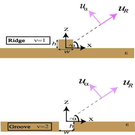
As represented in Fig. 1, we shall be expressing the source orientation in a cartesian basis $({\bf u}_{x},{\bf u}_{z})$, and the scattered fields in a right-handed orthogonal polar basis:

$${\bf u}_{R} = \cos\alpha{\bf u}_{x}+\sin\alpha{\bf u}_{z}$$ (1)

$${\bf u}_{\alpha} = -\sin\alpha{\bf u}_{x}+\cos\alpha{\bf u}_{z}$$ (2)

Finally a question of notation: throughout we shall refer to a bi-dimensional point-source simply as a dipole, but it is meant that their emission as all of the fields are cyclical in the $y$-direction. As represented in Fig. 1, each object lying in the vacuum semi-space shall be labeled by the superscript $\nu=1$ while any object lying in the metal shall be labeled by the superscript $\nu=2$. In particular, scattering quantities related to ridges have the superscript $\nu=1$ while the ones related to grooves have the superscript $\nu=2$. The field within the cross-sectional area of the ridge is labeled ${\bf E}^{r}({\bf r}^{\prime})$ and the one within that of the groove is labeled ${\bf E}^{g}({\bf r}^{\prime})$ .

III Scattering Coefficients

Figure 1: Schematic representation of the scattering systems considered. A ridge is a one dimensional defect located in air and labeled by the index $\nu=1$. A groove is a one dimensional defect located in the metal and labeled by the index $\nu=2$

The Green tensor approach is a standard method to solve electromagnetic scattering problems H.W.Hohmann (1975); Protásio et al. (1982); Keller (1986); Li et al. (1991); Martin et al. (1995); Felsen and Marcuvitz (2003); L.Novotny and B.Hecht (2006); Nikitin et al. (2008). Our first task in this section, is to arrive at an explicit expression for the scattered electric far-field. This is attained by propagating the field induced by a dipole density ${\bf P}^{(1)}({\bf r}^{\prime})=\Delta\varepsilon\;{\bf E}^{r}({\bf r}^{\prime})$ (where $\Delta\varepsilon=\varepsilon-1$) inside the area of a ridge, to a point ${\bf R}$ very far from the source. For a groove we have the same relation between polarization and field (except for a change of sign) ${\bf P}^{(2)}({\bf r}^{\prime})=-\Delta\varepsilon\;{\bf E}^{g}({\bf r}^{\prime})$. To propagate the field from any of the two, we use the standard formula L.Novotny and B.Hecht (2006):

$${\bf E}_{s}({\bf R})=g^{2}\int_{A}d{\bf r}^{\prime}{\bf\hat{G}}({\bf R},{\bf r}^{\prime})\cdot{\bf P}({\bf r}^{\prime}).$$ (3)

Where ${\bf\hat{G}}({\bf R},{\bf r}^{\prime})$ is the Green tensor for the air-metal background. The Green tensor propagates the emission of a point source at ${\bf r}^{\prime}$ to the distant point of the ${\bf R}$. One of the advantages of the Green tensor technique is that once the fields inside the defects ${\bf E}({\bf r}^{\prime})$ (and thus ${\bf P}({\bf r}^{\prime})$) are computed numerically the asymptotic expansions of scattered fields become analytic. This takes us to our second task, which is making a direct connection between the orientation of the induced polarization inside the defects and the far-field radiation pattern, and in so doing define the scattering coefficients.
First of all, finding the scattered electric far-field ${\bf E}_{s}({\bf R})$ requires the asymptotic expansions of the Green tensor. The derivation is sketched in the Appendix C. In what follows we give some simplifying rearrangements that will let us focus directly on the angular radiation pattern of surface defects.

III.1 Scattering into Radiative Modes

The asymptotic Green’s tensor in the radiative zone for either a ridge or a groove can be written in a compact form as:

$${\bf\hat{G}}^{(\nu)}(R\rightarrow\infty,\alpha,{\bf r}^{\prime}) = \,\frac{e^{i(gR+\pi/4)}}{\sqrt{8\pi gR}}\,e^{-igx^{\prime}\cos\alpha}\times$$ (4)

$$\times e^{-ik_{z}^{\nu}z^{\prime}}\;{\bf\hat{G}}_{\infty}^{(\nu)}(\alpha,{\bf r}^{\prime}).$$

In such form we can factor the asymptotic scalar green function out of the dyadic part of the Green tensor. From eq.(3), the direction of ${\bf E}_{s}({\bf R})$ results from superposition of ${\bf\hat{G}}_{\infty}^{(\nu)}(\alpha,{\bf r}^{\prime})\cdot{\bf P}^{\nu}({\bf r}^{\prime})$, the emission from all induced point polarization elements, or dipole density elements. Yet the direction of each contribution ${\bf\hat{G}}_{\infty}^{(\nu)}(\alpha,{\bf r}^{\prime})\cdot{\bf P}^{\nu}({\bf r}^{\prime})\,$ must be independent of ${\bf r}^{\prime}$. In other words since electromagnetic waves are transverse waves in vacuum, far from their source, the field emitted by a dipole ${\bf\hat{G}}_{\infty}^{(\nu)}(\alpha,{\bf r}^{\prime})\cdot{\bf P}^{\nu}({\bf r}^{\prime})$ must be proportional to ${\bf u}_{\alpha}$. In fact using the standard asymptotic expansions (see the Appendix C) we can write:

$${\bf\hat{G}}_{\infty}^{(\nu)}(\alpha,{\bf r}^{\prime})\cdot{\bf P}^{\nu}({\bf r}^{\prime})=-\left[{\bf\Phi}^{(\nu)}(\alpha,{\bf r}^{\prime})\cdot{\bf P}^{\nu}({\bf r}^{\prime})\right]\;{\bf u}_{\alpha}.$$ (5)

Where for a ridge:

$${\bf\Phi}^{(1)}(\alpha,z^{\prime})=\mbox{\boldmath${\bf k}$}_{p}^{+}(\alpha)+\mbox{\boldmath${\bf k}$}_{p}^{-}(\alpha)\>r_{p}(\alpha)\>e^{2igz^{\prime}\sin\alpha}.$$ (6)

and for a groove:

$${\bf\Phi}^{(2)}(\alpha)=t_{p}^{(1,2)}(\alpha)\,{\bf k}_{pm}(\alpha).$$ (7)

The vectors $\mbox{\boldmath${\bf k}$}_{p}(\alpha)$ are p-waves defined in vacuum, while $\mbox{\boldmath${\bf k}$}_{p}^{m\pm}(\alpha)$ are defined in the metal. A reminder of their expressions at normal incidence, in terms of the angle $\alpha$ of Fig. 1, is reported in the Appendix B, along with the expression for the Fresnel reflection and transmission coefficients: $r_{p}(\alpha)$, $t_{p}^{(1,2)}(\alpha)$.
We are now in a position to write the expressions for the radiative fields. Plugging eq.(4) and eq.(5) into eq.(3) we can separate the electric far field dependence into its radial and angular parts as:

$${{\bf E}}_{s}^{(\nu)}(R,\alpha)=-\,\frac{e^{i(gR-\pi/4)}}{\sqrt{8\pi gR}}\;E_{s}^{(\nu)}(\alpha)\;{\bf u}_{\alpha}.$$ (8)

Here the angular amplitude can be written as:

$$E_{s}^{(\nu)}(\alpha)=g^{2}\,\Theta_{rad}^{(\nu)}(\alpha)$$ (9)

where $\Theta_{rad}^{(\nu)}(\alpha)$ is the scattering coefficient into radiative-modes:

$$\Theta_{rad}^{(\nu)}(\alpha)=\int_{A}d{\bf r}^{\prime}\,e^{-igx^{\prime}\cos\alpha}e^{-ik_{z}^{(\nu)}z^{\prime}}{\bf\Phi}^{(\nu)}(\alpha,{\bf r}^{\prime})\cdot{\bf P}^{(\nu)}({\bf r}^{\prime})$$

(10)

In the last expression the scattered field in the far zone consists of a cylindrical wave, transverse to the direction of propagation ${\bf u}_{R}$, and with a net angular amplitude determined by the integral over the source region $\Theta_{rad}^{(\nu)}(\alpha)$. The latter is actually the important bit in the formula as its squared module determines the radiation pattern. As seen from eq.(10) this angular amplitude results from the superposition of each scattering element taken with its own amplitude, phase and optical path in analogy to how an antenna array determines its effective radiation pattern. The radiation is given by the intensity or Poynting vector in the far field. Accordingly the differential angular scattering cross-section is:

$$\frac{\partial\sigma_{rad}^{(\nu)}(\alpha)}{\partial\alpha} = \frac{|{{\bf E}}_{s}^{(\nu)}(R,\alpha)|^{2}R}{S_{spp}}=\frac{g^{3}}{S_{spp}}|\Theta_{rad}^{(\nu)}(\alpha)|^{2}.$$

Finally, the net radiative loss $\sigma_{rad}$ is defined as the integrated angular radiation:

$$\sigma_{rad}=\int_{0}^{180^{0}}d\alpha\;\frac{\partial\sigma_{rad}^{(\nu)}(\alpha)}{\partial\alpha}.$$ (12)

III.2 Shallow defects and Green’s tensor boundary conditions

Whenever the height of the defect is small enough, typically much smaller than the wavelength of the incident light, we can make the approximation $g|{\bf r}^{\prime}|<<1$. That allows for some simplification for the angular amplitude of a scattering element above the surface. Consider:

$${\bf\Phi}^{(1)}(\alpha,{\bf r}^{\prime}) = (\mbox{\boldmath${\bf k}$}_{p}^{+}(\alpha)+\mbox{\boldmath${\bf k}$}_{p}^{-}(\alpha)\>r_{p}(\alpha)\>e^{2igz^{\prime}\sin\alpha})\simeq$$ (13)

$$\simeq (\mbox{\boldmath${\bf k}$}_{p}^{+}(\alpha)+\mbox{\boldmath${\bf k}$}_{p}^{-}(\alpha))\>r_{p}(\alpha)$$

Hence, for shallow defects the Green Tensor dependence of eq.(4) is entirely given by the exponential factors $e^{-igx^{\prime}\cos\alpha}e^{-ik_{z}^{\nu}z^{\prime}}$, for both a source in the vacuum semi-space and a source in the metal semi-space. Indeed this turns out to be a major simplification for the relative amplitude of the scattering elements in the air semi-space, which we shall perform in detail SectionVI.
Before that we need to highlight the relation between the Green tensor of a defect on the metal slab and in the metal slab, under this approximation. Such relation emerges from the boundary conditions for the Green’s tensor at the interface, which are:

$${}\left[{\bf\hat{G}}({\bf R},x^{\prime},z^{\prime}=0^{+})-{\bf\hat{G}}({\bf R},x^{\prime},z^{\prime}=0^{-})\right]\cdot{\bf u}_{x}=0$$

$$\left[{\bf\hat{G}}({\bf R},x^{\prime},z^{\prime}=0^{+})-\varepsilon\,{\bf\hat{G}}({\bf R},x^{\prime},z=0^{-})\right]\cdot{\bf u}_{z}=0.$$

Notice that, in the unperturbed system, space is translationally invariant in the horizontal direction $x$ and this is reflected in is the $x$-component of the vector in eq.(13). Because of eq.(4) and eq.(5), we can turn eq.(III.2) into:

$$\Phi^{(1)}_{x}(\alpha)={\Phi}^{(2)}_{x}(\alpha)={\Phi}_{x}(\alpha).$$ (16)

The presence of surface charges at the interface implies, from eq.(III.2), that the $z$-components of the vector ${\bf\Phi}^{(\nu)}(\alpha)$ on either sides of the interface have the relation:

$$\Phi^{(1)}_{z}(\alpha)=\varepsilon\;{\Phi}^{(2)}_{z}(\alpha).$$ (17)

III.3 Scattering into Surface Plasmons

Let us derive the scattering coefficient into surface plasmon modes. Note that, in this one dimensional problem, scattering will be into both the forward surface plasmon ${\bf e}_{spp+}({\bf r})$, propagating in the positive $x$ direction and the backwards plasmon ${\bf e}_{spp-}({\bf r})$ propagating in the negative $x$ direction, as defined in the Appendix A. The emission by a point dipole or a point polarization element must result into a plasmon final state: ${\bf\hat{G}}_{p\pm}({\bf R},{\bf r}^{\prime})\cdot{\bf P}({\bf r}^{\prime})\propto{\bf e}_{spp\pm}$, as shown in the derivation sketched in the Appendix C. The asymptotic Greens tensor for a source upon ($\nu=1$) or in ($\nu=2$) the metal is:

$${\bf\hat{G}}_{p\pm}^{(\nu)}({\bf R},{\bf r}^{\prime})\cdot{\bf P}^{(\nu)}({\bf r}^{\prime}) =\frac{i}{2g\,S_{spp}}\times$$ (18)

$$\times\left[\,\left({\bf e}^{(\nu)}_{spp\pm}({\bf r}^{\prime})\right)^{*}\cdot{\bf P}^{(\nu)}({\bf r}^{\prime})\,\right] {\bf e}_{spp\pm}({\bf R}).$$

Notice that $\left({\bf e}^{(\nu)}_{spp\pm}({\bf r}^{\prime})\right)^{*}$ complies with eq.(III.2) and eq.(III.2). Consequently the field of the scattered plasmons are:

$${\bf E}_{p}^{(\nu)\pm} = -\frac{ig}{2\,S_{spp}}\Theta_{p\pm}^{(\nu)}\;{\bf e}_{spp\pm}$$

$$\Theta_{p\pm}^{(\nu)} = \int_{A^{(\nu)}}d{\bf r}^{\prime}\;{\bf e}^{*}_{spp\pm}({\bf r}^{\prime})\cdot{\bf P}({\bf r}^{\prime})$$ (19)

Furthermore the magnetic field related to the field scattered into SPPs is :

$${\bf H}_{p\pm}=-\frac{ig}{2\,S_{spp}}\,\Theta_{p\pm}\;{\bf h}_{spp\pm}$$ (20)

where ${\bf h}_{spp}$ is the magnetic field of a SPP, as proved in the Appendix A.
Now, if the the source ${\bf P}({\bf r}^{\prime})$ is produced by an incident surface plasmon field (as is our case), we can define the scattering cross-section of into SPPs as:

$$\sigma_{p}^{\pm}=\frac{{\bf E}_{p\pm}\times{\bf H}_{p\pm}^{*}\cdot{\bf u}_{x}}{{\bf e}_{p\pm}\times{\bf h}_{p\pm}^{*}\cdot{\bf u}_{x}}=\left|\frac{g}{2\,S_{spp}}\Theta_{p\pm}\right|^{2}$$ (21)

Finally, we can define the total scattering cross-section, which in the lossless case is equivalent to the extinction cross-section:

$$\sigma_{xtn}=\sigma_{p}^{+}+\sigma_{p}^{-}+\sigma_{rad}$$ (22)

IV Rayleigh-limit: cautionary remarks

Next we are going to develop solutions to point sources in a metal plane background. However one question may be raised : how do we associate the field induced by a surface plasmon inside a ridge or a groove to a point dipole? The answer is the argument of this section.
When the field inside a defect is obtained by mesh discretization we assume that the field inside a single mesh is uniform, and deviations from the field at its center are deemed negligible. Yet, in general, the field in a defect, cannot be represented by the field at its center alone. Let us explain a little bit further this point.
For simplicity let us consider a defect in a homogenous medium with dielectric constant $\varepsilon_{b}$, but the argument is the same in other backgrounds. As usualPaulus and Martin (2001), the field at every mesh is found by solving self-consistently a system of $N$ coupled equations:

$${\bf E}({\bf r}_{i})={\bf E}_{b}({\bf r}_{i})\;+\,g^{2}\,\sum_{j\neq i}{\bf\hat{G}}_{b}({\bf r}_{i}-{\bf r}_{j})\cdot\Delta\varepsilon\,{\bf E}({\bf r}_{j})\frac{A}{N^{2}}+$$

$$\,+g^{2}\>{\bf\hat{M}}\cdot\Delta\varepsilon\,{\bf E}({\bf r}_{i})-\frac{{\bf\hat{L}}}{\varepsilon_{b}}\cdot\Delta\varepsilon\,{\bf E}({\bf r}_{i})\;\;\;$$ (23)

where $i=1,N$ and $j=1,N$ and ${\bf E}({\bf r}_{i})$ is the field at the mesh center. ${{\bf\hat{L}}}$ is a term related to the depolarization of light and comes about from the quasi-static contribution of the Green tensor. ${{\bf\hat{M}}}$ is a correction term to the Green tensor in the region of the scatterer useful to improve the accuracy of the calculation, when the inhomogeneity is discretized L.Novotny and B.Hecht (2006); Martin and Piller (1998).
In practice, the number of mesh points $N$ is increased until the calculation converges to the required precision. Then scale variations $\sim\sqrt{A}/N$ of ${\bf E}({\bf r})$ are properly represented in the solution. In the Rayleigh limit, for a defect of area $A$ so small that $g^{2}A<<1$, the scatterer behaves like a point source or a point dipole and the background field (in this case the illumination) can be considered uniform over $A$: ${\bf E}_{b}({\bf r})={\bf E}_{b}$ . Exceptionally, for a circular defect in a homogenous medium with dielectric constant $\varepsilon_{b}$, the net field at any point ${\bf r}_{i}$ converges to:

$${\bf E}={\bf E}_{b}\;-\frac{{\bf\hat{L}}}{\varepsilon_{b}}\cdot\Delta\varepsilon\,{\bf E}\;\;\;$$ (24)

Figure 2: Dependence of the extinction coefficient on the number of meshes used in the calculation, for a square defect with $w=h=1nm$ in vacuum, and a circular defect of the same area, illuminated by a plane wave. The dashed line represents extinction coefficient calculated with the Mie theory for the circle. The dielectric constant in the defect is $\varepsilon=-19.89$ at the wavelength of $700nm$. The inset represents the geometry of a discretized circle when inscribed in a square represented by 30x30 mesh points.

This is because for the field inside an infinitesimal (very sub-wavelength) circular shape is actually uniform and thus scattering by such circular defects can be described by one mesh. In fact the extinction coefficientEvlyukhin et al. (2007); Søndergaard and Bozhevolnyi (2003) can be derived from the field at the center alone:

$$\sigma_{xtn} = g\Im\left[\int_{A}d{\bf r}^{\prime}\,\Delta\varepsilon{\bf E}^{*}_{b}({\bf r}^{\prime})\cdot{\bf E}({\bf r}^{\prime})\right]=$$ (25)

$$= A\Im\left[\Delta\varepsilon{\bf E}^{*}_{b}\cdot{\bf E}\right]$$ (26)

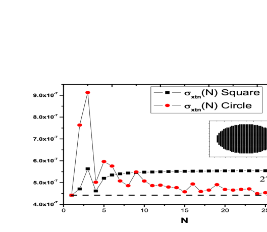
To prove this numerically we have calculated $\sigma_{xtn}$ for a cylinder represented by a single mesh, as in eq.(24), and illuminated by a plane wave. First of all we have checked that the one-mesh cross-section of eq.(26), coincides with the Mie theory result. Secondly, we have subdiscretized the cylinder into square meshes as rendered in the inset of Fig. 2. As also rendered in the figure, applying eq.(IV) we found that, as the number of meshes grows, the scattering cross-section calculated by the collection of meshes eq.(25) converges to the initial value of one single mesh of eq.(26). However the field inside of a square scatterer can never be uniform if it is to satisfy real boundary conditions even in a homogenous medium or vacuum. Thus, it can not be faithfully described by one mesh. This is illustrated in Fig. 2, which renders the extinction coefficient for a square defect of the same area as the circle. As it turns out, the converged value is $\sim 27\%$ larger than that obtained by the one-mesh approximation. Remarkably this error is not reduced with the defect size: we obtained the same error for squares with side $5nm$ or $0.5nm$. This is just for reference in the optical range, since we found that the error actually depends on type of defect and on the dielectric constant.
However, even if the field is not uniform, a small defect in the Rayleigh limit can be represented by a point source at the center of the mesh, with its field equal to the average field over the mesh $\overline{{\bf E}}=(1/A)\int_{A}d{\bf r}^{\prime}\,{\bf E}({\bf r}^{\prime})$.
Indeed if the variation of ${\bf E}_{b}({\bf r})$ is negligible over the area of the defect we have:

$$\sigma_{xtn}=A\Im\left[\Delta\varepsilon{\bf E}^{*}_{b}\cdot\overline{{\bf E}}\right]$$ (27)

So the object behaves as a point-dipole ${\bf p}=A\Delta\varepsilon\overline{{\bf E}}$.
The previous results were for a homogeneous background, but they also hold for the inhomogeneous one considered in this paper. We find that, for a defect above the surface in the optical range, the relative error is about $40\%$, while it can reach $50\%$ for a defects below the surface.
With very small non-elongated ridges and grooves, such that $w/\lambda\approx h/\lambda<<1$, the equivalent point dipoles are attained by averaging the fields over the area of the defects as follows:

$${\bf p}^{(1)} = \Delta\varepsilon\overline{{\bf E}}^{r}\,A=\Delta\varepsilon\int_{A}d{\bf r}^{\prime}\,{\bf E}^{r}({\bf r}^{\prime})$$ (28)

$${\bf p}^{(2)} = -\Delta\varepsilon\overline{{\bf E}}^{g}\,A=-\Delta\varepsilon\int_{A}d{\bf r}^{\prime}\,{\bf E}^{g}({\bf r}^{\prime})e^{-ig|z^{\prime}|\sqrt{|\varepsilon|}}.$$

Accordingly if we set ${\bf P}^{(\nu)}({\bf r})=\delta({\bf r}-{\bf r}^{\prime}){\bf p}^{(\nu)}$ eq.(10) and eq.(III.3) for small non-elongated defects become:

$$\Theta_{rad}^{(\nu)}(\alpha) = {\bf\Phi}^{(\nu)}(\alpha)\cdot{\bf p}^{(\nu)}$$ (30)

$$\Theta_{p\pm}^{(\nu)}(\alpha) = \left[{\bf e}_{p\pm}^{(\nu)}(0)\right]^{*}\cdot{\bf p}^{(\nu)}$$ (31)

V Numerical results

As an illustration consider a square ridge and a groove of side $w=h=10nm$. We have calculated the scattering into radiative modes and SPPs without associating the defect to a point dipole but rather using eq.(III.1) and eq.(21). In this case the major task is computing the Green’s tensor for the plane metal surface required to attain the exact field within the surface defect. This can be achieved following the prescriptions of Ref. [Paulus et al., 2000; Søndergaard and Bozhevolnyi, 2004].
Similar numerical results for the case of shallow grooves were found in Ref. [Chremmos, 2010] using a different computational technique.
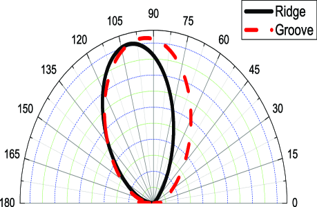
The out of plane radiation pattern of a surface plasmon scattered by such defects is given in Fig. 3.
Calculations show that, for symmetric defects, the net radiative loss is greater for a groove than for a ridge. This is so because, while both the scattering into SPPs and the radiation close to the surface (at $\alpha=0,180^{\circ}$) are similar, their radiation patterns greatly differ normal to the surface ($\alpha=90^{\circ}$), where the groove radiation is maximum while the ridge radiation goes to zero.

Figure 3: Angular radiative cross section (eq.(III.1)) and surface plasmon cross section (eq.(21) represented by the almost horizontal lines at $\alpha\simeq$ and $\alpha\simeq 180^{0}$), for square defects with 10nm side, illuminated by a SPP on silver at $500nm$. The scale is linear but the units are arbitrary. Each concentric line indicates an equal increment of the cross-sections, from the minimum at the the center to the maximum at the outermost.

Figure 4: Angular radiative cross section (eq.(III.1)) and surface plasmon cross section (eq.(21) represented by the almost horizontal lines at $\alpha\simeq$ and $\alpha\simeq 180^{0}$), for rectangular defects with $10nm$ height and 50nm width, illuminated by a SPP on silver at $700nm$. The scale is linear but the units are arbitrary. Each concentric line indicates an equal increment of the cross-sections, from the minimum at the the center to the maximum at the outermost.

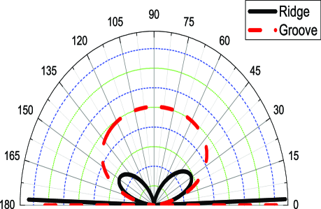
The ridge radiation pattern is distributed into two lobes on either sides of $\alpha=90^{\circ}$ but the groove radiation pattern forms a single lobe. This is one of our main result and shall be analyzed in detail in the next section. The result is not in agreement with those obtained in the approximate treatment Ref.[Nikitin et al., 2007]. We associate the discrepancy to the breakdown of the condition that the curvature of a short and shallow defect does not vary rapidly, used in that work.
Notice the fraction of energy scattered into SPPs, i.e $\sigma_{p}^{\pm}$ of eq.(21), is large. The values of $\sigma_{p}^{\pm}$ are represented by the horizontal lines of Fig. 3 (the concentric lines indicate their amplitude in a linear scale and in arbitrary units, say, for instance from $0$ at the center to $8$ at the outermost). For both ridges and grooves $\sigma_{p}^{+}$ and $\sigma_{p}^{-}$ are roughly equal. However in the case of ridges, $\sigma_{p}^{\pm}$ is greater than the maximum value of the scattering cross-section into radiative modes ${\partial\sigma_{rad}^{(1)}(\alpha)}/{\partial\alpha}$ of eq.(III.1), by a factor slightly greater than $2$. For grooves, $\sigma_{p}^{\pm}$ is greater than the maximum value of ${\partial\sigma_{rad}^{(2)}(\alpha)}/{\partial\alpha}$ by a factor slightly smaller than $2$.
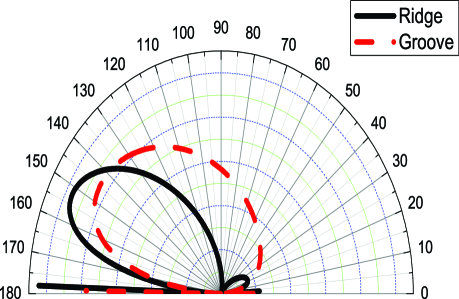
Let us now keep the defects height at $h=10nm$ and enlarge the width $w$. Fig. 4 renders the radiation pattern for a rectangular defect of width $50$nm ($h=10nm$). The emergence of directivity in the out of plane radiation, is part of a transitional behavior, in which the radiation patterns tend to align and, simultaneously, one of the lobes is shrunk while the other is blown up in the ridge radiation. Notice that the scattered energy into SPPs exhibits the same directivity, going mainly in reflection. Eventually, if we keep enlarging the defects until they are considerably asymmetric the radiation patterns for both ridges and grooves tend to be single overlapping lobes (see Fig. 5). Noticeably, the scattering into SPPs is greatly reduced. Such similarity is explainable in the approximate framework presented in Ref.[Nikitin et al., 2007] which turns out to be quite acceptable in this limit of large enough defects, as we shall substantiate in Sec. VII. In Sec. VIII we shall account qualitatively for the transition observed in Fig. 4, explaining why the radiation pattern changes when the defects are enlarged.

Figure 5: Angular radiative cross section (eq.(III.1)) and surface plasmon cross section (eq.(21) represented by the almost horizontal lines at $\alpha\simeq$ and $\alpha\simeq 180^{0}$), for rectangular defects with $10nm$ height and $300nm$ width, illuminated by a SPP on silver at $700nm$. The scale is linear but the units are arbitrary. Each concentric line indicates an equal increment of the cross-sections, from the minimum at the the center to the maximum at the outermost.

V.1 Scattering by square ridges and grooves in the Rayleigh limit

The equivalence between non-elongated subwavelength defects and point dipoles gives us a chance to investigate in depth the individual radiation pattern of a single scattering element.
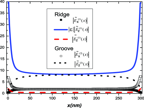
Fig. 6 shows the averaged the field inside the 10nm ridges and grooves, as prescribed in eq.(28) and eq.(IV). The field induced in a groove is mainly longitudinal while the field inside the ridge is mainly transversal. This is due to both the illumination and the polarizabilty of the scatterers. When defects are almost symmetric their polarizibilities $\beta_{i}$ are nearly isotropic and so the induced field and the incident field are virtually parallel. Hence the field induced in a ridge and a groove are nearly parallel to the incident surface plasmon ${\bf e}_{spp}$, which is mainly perpendicular to the plane in the vacuum semi-space and is mainly parallel to the plane in the metal semi-space. Therefore, in the Rayleigh limit, a ridge scatters SPPs into radiative modes like a vertical dipole on the plane, while the groove scatters them into radiative modes like a horizontal dipole on a plane. The results for grooves is in agreement with Ref.[Lévêque et al., 2007].
Interestingly, we also have found numerically in Fig. 6 that:

$$|\overline{E}_{x}^{g}|\sim|\sqrt{\varepsilon}\;\;\overline{E}_{z}^{r}|$$ (32)

especially at short wavelengths. We have devised a virtual source, that can condense the orientation of the equivalent dipole representing a non-elongated symmetric ridges and grooves. This virtual dipole is defined as: ${\bf q}(\theta)={\bf u}_{x}\sqrt{|\varepsilon|}\cos\theta+{\bf u}_{z}\sin\theta$. The fields inside a groove and a ridge, are respectively, represented as:

$$|\overline{{\bf E}}^{g}| \simeq |\Delta\varepsilon\,\overline{E}^{r}_{z}{\bf q}(0)|$$ (33)

$$|\overline{{\bf E}}^{r}| \simeq |\Delta\varepsilon\,\overline{E}^{r}_{z}{\bf q}(90^{0})|$$ (34)

at least as long as eq.(32) holds.
In reality we can see what happens by means of eq.(24). Despite the fact that this equation is only exact for a circle in a homogenous background (as explained) we can use it to show qualitatively the relation between the field inside the groove and the ridge, when their shapes are symmetric. If we approximate the polarizability of a ridge for that of a circle in vacuum (whose polarizability is calculated through eq.(24)), so $\beta_{1}=2/(\varepsilon+1)$. If we also approximate the groove polarizability by that of a hole in a homogenous metal medium, we have: $\beta_{2}=2\varepsilon/(\varepsilon+1)$. Hence the field induced inside each object is:

$$\overline{{\bf E}}^{r} \approx \beta_{1}{\bf e}_{spp}(x=0,z=0^{+})=\beta_{1}{\bf u}_{z}$$ (35)

$$\overline{{\bf E}}^{g} \approx \beta_{2}{\bf e}_{spp}(x=0,z=0^{-})=\beta_{2}\frac{{\bf u}_{x}}{\sqrt{\varepsilon}}$$ (36)

Since these polarizabilities also have the property: $\beta_{2}=\varepsilon\beta_{1}$ (the polarizability of a hole in a material is $\varepsilon$ times larger than the polarizability of a particle of the same material and the same shape) then $|\sqrt{\varepsilon}\;\overline{E}^{g}_{x}|\sim|\overline{E}^{r}_{z}|$.

Figure 6: The averaged field components (as defined in eq.(28), eq.(IV)) for a square groove and a square ridge of 10nm side in silver, as a function of the wavelength. The scale is logarithmic with arbitrary units.

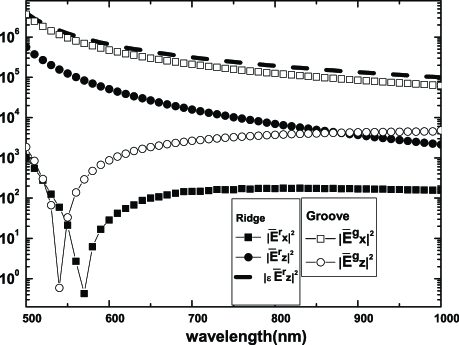
The symmetry of the polarizations $\beta_{i}$ and the property $\beta_{2}\simeq\varepsilon\beta_{1}$ are strictly true for circular defects in homogeneous media. Our numerical calculations of Fig. 6 shows that, even though the field inside a ridge and a groove are quantitatively different from those of circular defects in homogenous media, the assumption that their mutual relation is preserved is in very good agreement with the exact result. Because of the symmetry of the square shape, the averaged field inside the square is very nearly parallel to the incident field.

V.2 Reflection of surface plasmons square shallow defects

As a corollary of the properties of the fields in a ridge and a groove $|\sqrt{\varepsilon}\overline{E}^{r}_{z}|\sim|\overline{E}^{g}_{x}|$ we can also substantiate that their reflection of surface plasmons is quite similar. In fact, we obtain:

$$|E_{p\pm}^{(1)}|\simeq|\overline{E}^{r}_{z}|$$ (37)

$$|E_{p\pm}^{(2)}|\simeq\left|\frac{\overline{E}^{g}_{x}}{\sqrt{\varepsilon}}\right|\simeq|{\overline{E}^{r}_{z}}|\simeq|E_{p\pm}^{(1)}|$$ (38)

Notice that these define $\sigma_{p}^{\pm}$ through eq.(21). Once $\sigma_{rad}$ from eq.(12) and $\sigma_{p}^{-}$ are determined the value of the transmission of the surface plasmon is a constrained variable: $T=1-\sigma_{p}^{-}-\sigma_{rad}$, at least for the lossless caseNikitin et al. (2007). Since $\sigma_{rad}$ is greater for grooves than for ridges, the groove transmission is smaller.

VI Radiation patterns for Horizontal and Vertical point dipoles on a real metal interface

The first part of the expression eq.(III.1) is a pre-factor ${g^{3}}/{S_{spp}}$ whereas the second part is the the radiation pattern of a point dipole:

$$|\Theta^{(\nu)}|^{2}=\left|{\bf\Phi}^{(\nu)}(\alpha)\cdot{\bf p}\right|^{2}$$ (39)

A groove emits like a horizontal dipole. The angular amplitude of the field radiated by a horizontal unit dipole ${\bf p}={\bf u}_{x}$, placed close to the interface $z=0$, is ${\Phi}_{x}(\alpha)$, and it does not matter on which side of the interface it is placed. ${\Phi}_{x}(\alpha)$ can be derived using the relations in the Appendix B.2 and the explicit result is:

$${\Phi}_{x}(\alpha)=\frac{2\sqrt{\varepsilon-\cos^{2}\alpha}\;\sin\alpha}{\sqrt{\varepsilon-\cos^{2}\alpha}+\varepsilon\sin\alpha}$$ (40)

and the radiation pattern is $|{\Phi}_{x}(\alpha)|^{2}$. Notice ${\Phi}_{x}(\alpha)$ presents a mirror symmetry about the angle $\alpha=90^{0}$, the normal to to the plane. Furthermore since ${\Phi}_{x}(\alpha)$ never changes sign between $0$ and 180⁰ (nor goes to zero), the field of a horizontal dipole has one single symmetric lobe, where the field always has the same sign.

Figure 7: Radiative angular intensity $|\Phi_{x}|^{2}$ of a horizontal point dipole at an air-metal interface. The radiation patterns varies as the metal dielectric constant is varied. The scale is logarithmic with arbitrary units.

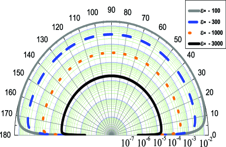
The field intensity $|{\Phi}_{x}(\alpha)|^{2}$ of such lobe is rendered in Fig. 7 for different dielectric constants. This radiation pattern of a groove shown in Fig. 7, is in agreement with the one represented by Ref.[Chremmos, 2010], obtained with a different numerical method. Notice that for $|\varepsilon|>>1$:

$${\Phi}_{x}\rightarrow 2\;{{\varepsilon}^{-1/2}}.$$ (41)

That is, when $\varepsilon$ increases this radiation pattern tends to become simultaneously isotropic and vanishing. In fact a horizontal dipole does not radiate on a perfect conductorSommerfeld (1964). On a small digression it is interesting to notice an apparent contradiction between treatments such as Ref.[H.A.Bethe, 1942], which considered that a defect in a perfect metal were equivalent to a magnetic dipole, while another workLévêque et al. (2007) explains a defect in a real metal corresponds to an electric dipole. Actually we have just reconciled the two results. We know that a horizontal dipole on a plane tends to emit isotropically for large $\varepsilon$. This means that on a first order expansion in $1/\varepsilon$, the radiation pattern of a horizontal dipole on a plane and that of a magnetic dipole in vacuum, are identical.
For finite $\varepsilon$ the field ${\Phi}_{x}(\alpha)$ of a horizontal dipole within a real metal would not be thoroughly screened, and while the pattern remains symmetric, its isotropy is disrupted parallel to the surface (i.e. $\alpha=0,180^{0}$) to accommodate the emergence of the surface plasmons density of states.
For an individual vertical dipole ${\bf p}={\bf u}_{z}$, which represents a ridge, the angular amplitude of the field is (see Appendix B.2) :

$${\Phi}_{z}^{(1)}(\alpha)=\frac{2|\varepsilon|\sin\alpha}{\sqrt{\varepsilon-\cos^{2}\alpha}+\varepsilon\sin\alpha}\;\;\large\cos\alpha$$ (42)

The field from a vertical dipole also goes to zero at $\alpha=0,180^{0}$ for a finite $\varepsilon$, but since dipoles only radiate transversally, the field has a third zero at $90^{0}$. The field is antisymmetric with respect to the normal of the plane, while the intensity $|{\Phi}_{z}(\alpha)|^{2}$ is symmetric, and is made up of the two lobes separated by a zero at 90⁰, see Fig. 8. Yet it is important to keep in mind that the field of one lobe is in anti-phase with the field of the other.

Figure 8: Radiation pattern $|\Theta_{rad}(\alpha)|$ from the virtual dipole $q(\theta)$ at $\theta=0,45^{0},90^{0}$. The scale is linear with arbitrary units.

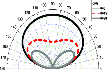
Unlike a horizontal dipole, the vertical dipole radiative field does not vanish for $|\varepsilon|>>1$ in fact:

$${\Phi}_{z}^{(1)}\rightarrow 2\cos\alpha$$ (43)

The total radiation from a vertical dipole has a larger weight than the radiation by a horizontal one, by a factor of $\sqrt{\varepsilon}$. This can be seen, in fact, from eq.(40) if we assume $\varepsilon$ is large, we get the following relation:

$$\Phi_{z}^{(1)}(\alpha)\simeq\sqrt{\varepsilon}\,\;{\Phi}_{x}(\alpha)\cos\alpha$$ (44)

In Fig. 8 we represent radiation pattern of ${\bf q}(\theta)$ for the horizontal and vertical orientations respectively, $\theta=0$, $\theta=90^{0}$, which corresponds to our analytic analog of the emission pattern of square ridges and grooves respectively. While we will consider an intermediate orientation in the next section, we want to remark here that, due to eq.(44), the radiation by both the horizontal moment ${\bf q}(0)$ and a vertical moment ${\bf q}(90^{0})$ vanish parallel to the plane at $\alpha=0,180^{0}$ in a similar manner, as illustrated in Fig. 3
At the same time the far-field emissions of ridges and grooves become increasingly different as we approach the direction normal to the plane.

VII Solutions for long and shallow Ridges and Grooves

For shallow and long defects $w>h$ and $h/\lambda<<1$ we define the following height-averaged polarization densities and fields:

$${\bf\widetilde{P}}^{(1)}(x^{\prime}) = \Delta\varepsilon\int_{0}^{h}dz^{\prime}{\bf E}^{(1)}(x^{\prime},z^{\prime})=$$ (45)

$$= \Delta\varepsilon\;\widetilde{{\bf E}}^{(1)}(x^{\prime})\;h$$

where the last equation defines ${\widetilde{{\bf E}}}^{(1)}(x^{\prime})$. Likewise for a groove we can define ${\bf\widetilde{P}}^{(2)}(x^{\prime})$ and $\widetilde{{\bf E}}^{(2)}(x^{\prime})$ through the following equation :

$${\bf\widetilde{P}}^{(2)}(x^{\prime}) = -\Delta\varepsilon\int_{-h}^{0}dz^{\prime}{\bf E}^{(2)}(x^{\prime},z^{\prime})\;e^{-g|z^{\prime}|\sqrt{|\varepsilon|}}$$ (46)

$$= -\Delta\varepsilon\;\widetilde{{\bf E}}^{(2)}(x^{\prime})\;h$$

Notice for $|\varepsilon|>>1$ we can make the approximation $k_{pz}^{m}\sim k_{z}^{m}\sim ig\sqrt{\varepsilon}$.
The benefit of using ${\bf\widetilde{P}}^{(\nu)}(x^{\prime})$ is that the scattered-field coefficients for these defects in the far zone, $\Theta_{rad}^{(\nu)}(\alpha)$ and $\Theta_{p\pm}^{(\nu)}$, are those emitted by a chain of point-dipoles on the surface over the segment $w$, and set at $0^{+}$ and $0^{-}$ for ridges and grooves, respectively.
The scattered field angular amplitude $\Theta_{rad}^{(\nu)}(\alpha)$ from eq.(10) and eq.(13) is obtained as:

$$\Theta_{rad}^{(\nu)}(\alpha) \simeq {\bf\Phi}^{(\nu)}(\alpha)\cdot\int_{0}^{w}d{\bf r}^{\prime}\,{\bf\widetilde{P}}^{(\nu)}(x^{\prime})\,e^{-igx^{\prime}\cos\alpha}$$ (47)

Figure 9: The averaged fields component inside of a ridge and a groove, $\widetilde{E}^{(1)}_{x}$, the quantity $\varepsilon\widetilde{E}^{(1)}_{z}$ and the rest of the components $\widetilde{E}^{(1)}_{x}$, $\widetilde{E}^{(2)}_{x}$, $\widetilde{E}^{(2)}_{z}$, for rectangular defects of $w=300nm$ and $h=10nm$. The system is illuminated by a SPP in lossless silver at $\lambda=700$nm. The scale is linear with arbitrary units.

This holds for the scattering into surface plasmon modes as well since we have:

$$\Theta_{p\pm}^{(\nu)} = \left[{\bf e}_{spp\pm}^{(\nu)}(0)\right]^{*}\cdot\int_{0}^{w}dx^{\prime}\;e^{\mp ik_{px}x^{\prime}}\;{\bf\widetilde{P}}^{(\nu)}(x^{\prime}).$$ (48)

When we illuminate a shallow and long defect, with a SPP, an equivalent linear density of dipole sources ${\bf\widetilde{P}}(x^{\prime})$ stems from how the induced fields are distorted inside the scatterer, namely by its polarizability. When the defect is larger in the horizontal direction than in the vertical one, ridges and grooves were found to give the same scattering by an approximated Rayleigh expansionNikitin et al. (2007). We have an alternative first principles argument to justify the Rayleigh expansion result, which is based entirely on the assumption that these defects are needle shaped. The field induced in these defects tends to be that induced in a needle-shaped protrusion placed horizontally on the surface $0^{+}$ in the case of a ridge. For a groove we have a horizontal needle-shaped cavity at $0^{-}$. In such idealistic simplification it is clear-cut to deduce the fields inside the defects from the boundary conditions. Namely the parallel component of the incident field is always continuous and equal, as in eq.(60)and eq.(61):

$$\widetilde{E}_{1x}(x^{\prime})={\bf e}_{sp}(x^{\prime},0)\cdot{\bf u}_{x}=\widetilde{E}_{2x}(x^{\prime})$$ (49)

which preserves the continuity of eq.(III.2). However, we are generating fields which, normal to the surface, make up for the discontinuity perpendicular to the metal surface of eq.(III.2). In fact, for a horizontal needle-like ridge, the boundary conditions imposed by the continuity of the displacement vector are:

$$\widetilde{E}_{1z}(x^{\prime})={\bf e}_{spp}(x^{\prime},0^{+})\cdot{\bf u}_{z}/\varepsilon=1/\varepsilon$$ (50)

while for a needle-like slit:

$$\widetilde{E}_{2z}(x^{\prime})=\varepsilon\;{\bf e}_{spp}(x^{\prime},0^{-})\cdot{\bf u}_{z}=1.$$ (51)

Ultimately:

$$\widetilde{E}_{1x}(x^{\prime}) = \widetilde{E}_{2x}(x^{\prime})$$ (52)

$$\varepsilon\widetilde{E}_{1z}(x^{\prime}) = \widetilde{E}_{2z}(x^{\prime})$$ (53)

which, matched with eq.(III.2) and eq.(III.2), yields:

$$\left|{\bf\hat{G}}({\bf R},x^{\prime},z^{\prime}=0^{+})\cdot\widetilde{{\bf E}}_{1}(x^{\prime})\right|=$$ (54)

$$=\left|{\bf\hat{G}}({\bf R},x^{\prime},z^{\prime}=0^{-})\cdot\widetilde{{\bf E}}_{2}(x^{\prime})\right|$$

and thus the property of producing the same scattering coefficients, previously found in Ref.[Nikitin et al., 2007]. Of course this is just an approximation, but it explains why elongated defects have similar scattering properties. In real life the plasmon scattering by protrusions and indentations is similar because, far from the edges, a shallow but elongated defect behaves as an infinitely elongated one, as confirmed by numerical calculations. As an example we report in Fig. 9 a numerical calculation of the fields averaged over the height for defects of $w=300nm$ and $h=10nm$. This shows that eq.(52) and eq.(53) are quite accurate at the center of the defect, and deviate from the needle model prediction due to fringe effects at the edges.
It is worth mentioning that this equivalence is valid in the Rayleigh limit when the defect size is much smaller than the wavelength, and may be altered at resonant wavelengths.

VIII The transition from short and shallow defects to long and shallow defects: oblique dipoles on a real metal plane

Everything we just said for symmetric surface defects was based on the fact that their aspect ratio equals one. As the defect width is increased, the aspect ratio becomes larger and this leads, progressively, to an asymmetric polarizability tensor. The first effect is that the field induced is gradually less and less parallel to the incident field. Therefore a ridge would develop a non-negligible horizontal electric field component, thus ceasing to be equivalent to a vertical dipole. Likewise the groove, which in the symmetric case behaves as a horizontal dipole, gradually starts having a non-negligible vertical component as its shape is elongated. The process goes on until we recover the case of a needle shaped defect of section VII. The fields inside a defect having intermediate width, as in Fig. 4, are intermediate between those for the needle case and the square symmetric case. Therefore in these cases defects emit qualitatively like oblique dipoles, with the orthogonal components out of phase.
In order to understand better the radiation pattern by ridges and grooves we decompose the oblique dipole in its horizontal and vertical components.
First of all, we focus on the mechanisms involved radiation pattern for a ridge $\nu=1$. From eq.(30) a dipole with arbitrary orientation emits close to the surface, with a field angular amplitude:

$$\Theta_{rad}^{(1)}(\alpha)={\bf\Phi}^{(1)}(\alpha)\cdot{\bf p}^{(1)} = {\Phi}_{x}(\alpha)\Delta^{(1)}(\alpha)$$ (55)

where $\Delta^{(1)}(\alpha)=p_{x}^{(1)}+\left({\Phi}_{z}^{(1)}(\alpha)/\Phi_{x}(\alpha)\right)\,p_{z}^{(1)}$ and equals:

$$\Delta^{(1)}(\alpha)=p_{x}^{(1)}+i\,\frac{\varepsilon\cos\alpha}{\sqrt{\cos^{2}\alpha+|\varepsilon|}}\,p_{z}^{(1)}$$ (56)

$\Delta^{(1)}(\alpha)$ shows that the contribution to the radiative field coming from the vertical and horizontal dipole on a metal plane have a phase difference of $90^{0}$. This was already evident from eq.(44), when $\varepsilon<0$. Such phase difference arises from the impedance of a metal planeNikitin et al. (2007) $Z_{s}=-i/{\sqrt{|\varepsilon|}}$.
The radiation pattern for a dipole with arbitrary orientation and lying above the metal, is written in our formalism as: $|{\Phi}_{x}(\alpha)\Delta^{(1)}(\alpha)|^{2}$.

Figure 10: Radiation pattern $|\Theta_{rad}(\alpha)|$ for a point dipole: ${\bf p}={\bf u}_{x}e^{i\phi}+{\bf u}_{z}$, lying on top of a metal surface. The scale is linear with arbitrary units.

The net angular amplitude for an oblique dipole is resolved into the superposition of the angular envelope of the horizontal dipole (shown in Fig. 7), with the other radiation factor $|\Delta^{(1)}(\alpha)|^{2}$. This last factor contains both the orientation and phase of the field. To envisage how these combine we may develop $|\Delta^{(1)}(\alpha)|^{2}$ into three terms. These consist in the individual emission from the horizontal and vertical dipole plus an interference term:

$$|\Delta^{(1)}(\alpha)|^{2}=|p_{x}|^{2}+\frac{|\varepsilon|^{2}\,\cos^{2}\alpha}{|\varepsilon|+\cos^{2}\alpha}|p_{z}|^{2}+$$

$$-2\;\frac{|\varepsilon|}{\sqrt{\cos^{2}\alpha+|\varepsilon|}}\;\Im\left[p_{1x}p_{z}^{*}\right]\cos\alpha$$ (57)

In the presence of the plane metal background, we have that horizontal and vertical dipoles behave as individual sources but their interaction presents an intrinsic added phase difference of $90^{0}$, which is due to the different interaction of a horizontal and a vertical dipole with the plane. As a result, when in phase they do not interfere, and their radiation pattern is always symmetric regardless of the orientation of the dipole. This is the case for ${\bf q}(45^{0})$ where, as in Fig. 8, the radiation pattern is the sum of the angular intensity of a vertical and a horizontal dipole, so that at $90^{0}$ there is a minimum due to the vanishing of the vertical dipole contribution, and yet never goes to zero because of the horizontal dipole contribution. Nevertheless, when the dipole components are not in phase, we can get asymmetric radiation patterns and additional zeros (to those at $0^{0}$ and $180^{0}$), because the interaction term can be negative. In such case the interaction of the horizontal radiative field (with only one lobe) with the vertical radiative (with two lobes of different sign) is responsible for an asymmetric radiation pattern and exhibits directionality.

Figure 11: Radiation pattern $|\Theta_{rad}(\alpha)|$ for a point dipole: ${\bf p}=\varepsilon{\bf u}_{x}+e^{i\phi}{\bf u}_{z}$, lying on top of a metal surface. The scale is linear with arbitrary units.

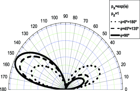
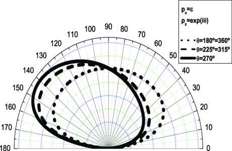
This is illustrated in Fig. 10 for a dipole emission whose main contribution comes from the vertical dipole. In Fig. 11 we show the radiation pattern for a dipole whose main contribution comes from the horizontal dipole radiation.
For the case of a grooves ($\nu=2$), the radiative angular field amplitude is, from eq.(17):

$$\Theta_{rad}^{(2)}(\alpha) = \Phi_{x}(\alpha)\Delta^{(2)}(\alpha)\;e^{-g|z^{\prime}|\sqrt{|\varepsilon|}}$$ (58)

$$\Delta^{(2)}(\alpha) = p_{x}^{(2)}+i\;\frac{\cos\alpha}{\sqrt{\cos^{2}\alpha+|\varepsilon|}}\;p_{z}^{(2)}$$ (59)

where remember we have also added the approximation: $k_{z}^{m}\simeq g\sqrt{\varepsilon}$ for $|\varepsilon|>>1$.
Remarkably, as opposed to the the dipole emission over the surface, in the net emission from a dipole under the surface the horizontal dipole contribution has a greater weight than the vertical dipole contribution. Apart from this, all the arguments used for a dipole over the surface apply.
The interaction between the vertical and horizontal components of the field induced in the field generates the directional patterns of Fig. 4. For a ridge with length slightly larger than its height the directional radiation is dominated by its vertical component. Fig. 10 exemplifies the effect of the interference of a dominant vertical component with a smaller but non-negligible horizontal component. For even larger aspect ratios the contribution from the other component may be comparable.
Likewise when a groove has a small aspect ratio it is predominantly a horizontal source interfering with a smaller vertical source. The result is in an interference pattern that looks like the one rendered in Fig. 11. Yet again this can be modified by increasing the aspect ratio. This transition is in good agreement with Fig. 11 of Ref.[Chremmos, 2010] where, using a different numerical method, the radiation pattern of a groove was computed for different aspect ratios.

IX Conclusions

Our analysis of the surface plasmon scattering by square shallow defects into radiative modes and plasmon modes, reveals that a groove scatters more of the incident energy than a ridge does. The reflection by a symmetric ridge and a groove is similar and so is the radiative emission close to the horizontal direction. Indeed their scattering essentially differs in the vertical direction, where a groove scatterers while a ridge does not. When defects start to become longer in width we saw the polarizability gets more asymmetric. Correspondingly, since both components of the incident plasmon are out of phase, defects are equivalent to interfering horizontal and vertical dipoles on a plane, which interfere constructively in some direction, thus producing directionality in the radiation pattern. Finally when ridges and grooves are shallow and long they tend to produce the same scattering as, apart for fringe effects, their polarizability exactly counterbalances the discontinuity of the incident surface plasmon field at the air-metal interface.

X Acknowledgments

The authors acknowledge financial support from the Spanish Ministry of Science and Innovation under grants NO.AP2005-5185, MAT2008-06609-C02 and CSD2007-046-Nanolight.es.

Appendix A Surface Plasmon Polariton Mode

The incident illumination is the field of a surface plasmon wave mode propagating in the positive x direction $(+)$ or negative x direction $(-)$ is:

$${\bf e}_{spp\pm}^{(\nu=1)}(\mathbf{r})=\left(\frac{\pm{\bf u}_{x}}{\sqrt{\varepsilon}}+{\bf u}_{z}\right)\;e^{i(\pm k_{p}x+k_{pz}z)},\;\;\;z>0,\;\;$$ (60)

$${\bf e}_{spp\pm}^{(\nu=2)}(\mathbf{r})=\left(\frac{\pm{\bf u}_{x}}{\sqrt{\varepsilon}}+\frac{{\bf u}_{z}}{\varepsilon}\right)\;e^{i(\pm k_{p}x+k_{pz}^{m}|z|)},\;\;\;z<0.\;\;$$ (61)

where $k_{p}=g(\varepsilon/(\varepsilon+1))^{1/2}$, $k_{pz}=ig/\sqrt{-\varepsilon-1}$ and $k_{pz}^{m}=-\varepsilon k_{pz}$. This can, alternatively, be written as: ${\bf e}_{spp\pm}({\bf r})={\bf e}_{spp\pm}^{(\nu=1)}$ for $z>0$; and ${\bf e}_{spp\pm}({\bf r})={\bf e}_{spp\pm}^{(\nu=2)}$ for $z<0$.
The magnetic field associated is continuous at the interface and equal to:

$${\bf h}_{spp\pm}({\bf r}) = \frac{-i}{g}\nabla\times{\bf e}_{spp\pm}({\bf r})$$ (62)

Now consider a lossless metal, characterized by a real and negative dielectric constant $\varepsilon$ and consider a plasmon moving in the forward direction, (the subscript + will be omitted). The incident Poyinting vector of the plasmon in the air side is:

$${\ S}_{spp}^{\nu=1}=\int_{0}^{\infty}dz\;{\bf e}_{spp}\times{\bf h}_{spp}^{*}\cdot{\bf u}_{x}=\;\frac{k_{p}}{g}\>\frac{Z_{s}^{2}+1}{2|k_{pz}|}$$ (63)

while in the metal is ${S}_{spp}^{\nu=2}=\int_{-\infty}^{0}dz\>{\bf e}_{spp}\times{\bf h}_{p}^{*}\cdot{\bf u}_{x}=Z_{s}^{4}{S}_{spp}^{\nu=1}$ where $Z_{s}=-i/\sqrt{|\varepsilon|}$. The total Poynting vector energy flux associated to a plasmon mode in a lossless metal is:

$${S}_{spp} = {S}_{spp}^{\nu=1}+{S}_{spp}^{\nu=2}=\frac{\sqrt{-\varepsilon}}{2g}\frac{(\varepsilon+1)(\varepsilon^{2}-1)}{\varepsilon^{3}}\geq 0.\>$$

Appendix B P-Modes

We shall repeat, out of completeness, the explicit expression for p-waves, particularly in the far field when $\mbox{\boldmath${\bf k}$}/g={\bf u}_{r}$. In this case these modes are expressed in terms of the direct space polar angle $\alpha$ by noticing that $k_{x}=g\cos\alpha$ and $k_{z}=k_{z}^{(\nu=1)}=g\sin\alpha$ in the air semi-space and $k_{z}^{m}=k_{z}^{(\nu=2)}=g\sqrt{\varepsilon-\cos\alpha^{2}}$ in the metal. Hence

$${\bf k}_{p}^{\pm}(\alpha) = \frac{1}{g}\left(k_{z}{\bf u}_{x}\mp k_{x}{\bf u}_{z}\right)=\sin\alpha{\bf u}_{x}\mp\cos\alpha{\bf u}_{z}$$

$$\mbox{\boldmath${\bf k}$}_{p}^{m\pm}(\alpha) = \frac{1}{\sqrt{\varepsilon}g}\left(k_{z}^{m}{\bf u}_{x}\mp k_{x}{\bf u}_{z}\right)=$$ (64)

$$= \sqrt{\frac{|\varepsilon|+\cos^{2}\alpha}{|\varepsilon|}}{\bf u}_{x}\mp\frac{\cos\alpha}{\sqrt{\varepsilon}}{\bf u}_{z}$$

B.1 Reflection and Transmission coefficients for a plane surface

For reference, we give here the Fresnel coefficients for an air metal interface. In the present treatment we only deal with the reflection coefficient for a p-wave propagating from air to metal, and this is :

$$r_{p}=r_{p}^{(1,1)} = \frac{k_{z}^{m}-\varepsilon\,k_{z}}{k_{z}^{m}+\varepsilon\,k_{z}}$$ (65)

where notice that, for the sake of tidiness, we omit the superscript throughout.
As to the transmission coefficients the one for a wave (2,1) propagating from the metal to air is $t_{p}^{(2,1)}$, while the one for a p-wave transmitted from the air medium to the metal is $t_{p}^{(1,2)}$.

$$t_{p}^{(2,1)}=\frac{2k_{z}^{m}\sqrt{\varepsilon}}{k_{z}^{m}+\varepsilon\,k_{z}}\;\;\;\;\;t_{p}^{(1,2)}=\frac{2k_{z}\sqrt{\varepsilon}}{k_{z}^{m}+\varepsilon\,k_{z}}$$ (66)

Notice that the transmission coefficients are related as follows:

$$\frac{t_{p}^{(1,2)}}{k_{z}^{(1)}}=\frac{t_{p}^{(2,1)}}{k_{z}^{(2)}}$$ (67)

B.2 Key Identities

The following expressions for the reflection and transmission coefficients are essential to derive eq.(40) and eq.(42):

$$t_{p}^{(1,2)}(\alpha)=\frac{2\sqrt{\varepsilon}\sin\alpha}{\sqrt{\varepsilon-\cos^{2}\alpha}+\varepsilon\sin\alpha}$$ (68)

$$1+r_{p}(\alpha)=\frac{2\sqrt{\varepsilon-\cos^{2}\alpha}}{\sqrt{\varepsilon-\cos^{2}\alpha}+\varepsilon\sin\alpha}$$ (69)

$$1-r_{p}(\alpha)=\frac{2\varepsilon\sin\alpha}{\sqrt{\varepsilon-\cos^{2}\alpha}+\varepsilon\sin\alpha}$$ (70)

Appendix C Asymptotic Green’s Tensors

The asymptotic expressions for the Green tensor for $3$D scatterers are found in referencesEvlyukhin et al. (2007); Novotny (1997); L.Novotny and B.Hecht (2006). We have already presented the derivation scheme for bi-dimensional defects in Appendix B of Ref.[Nikitin et al., 2008], for a groove. As explained therein the Surface plasmon Green tensor and the far-field Green tensor are obtained from its angular spectrum. From the relevant Sommerfeld integral the surface plasmon contribution is obtained by applying the residue theorem and the far-field Green tensor instead is obtained by applying the method of the steepest descent.
For the case of the ridge we use the total Green tensor of the background in the vacuum semi-space. This can be written as the sum of the direct Green Tensor (the free space green tensor ) and the indirect green tensor (which gives the contribution due to the reflections at the metal plane interface). Hence

$${\bf\hat{G}}^{(1)}({\bf R},{\bf r}^{\prime})={\bf\hat{G}}_{0}({\bf R},{\bf r}^{\prime})+{\bf\hat{G}}_{s}({\bf R},{\bf r}^{\prime})$$ (71)

where the spectral representation for the direct Green tensor is:

$${\bf\hat{G}}_{0}({\bf R},{\bf r}^{\prime}) = \frac{i}{4\pi}\int^{\infty}_{-\infty}\frac{dk_{x}}{k_{z}}\>e^{ik_{z}(Z-z^{\prime})}{e^{ik_{x}(X-x^{\prime})}}\>\mbox{\boldmath${\bf k}$}_{p}^{+}\mbox{\boldmath${\bf k}$}_{p}^{+},$$

while for the indirect Green Tensor:

$${\bf\hat{G}}_{s}({\bf R},{\bf r}^{\prime})=\frac{i}{4\pi}\int^{\infty}_{-\infty}\frac{dk_{x}}{k_{z}}\>{e^{ik_{x}(X-x^{\prime})}}e^{ik_{z}(Z+z^{\prime})}r_{p}\>\mbox{\boldmath${\bf k}$}_{p}^{-}\mbox{\boldmath${\bf k}$}_{p}^{+}.$$

Applying the residue theorem and the steepest descent method to ${\bf\hat{G}}^{(1)}({\bf R},{\bf r}^{\prime})$ we end up with eq.(4) and eq.(18) for ($\nu=1$).
For the groove case we need to expand the Green Tensor connecting a point in the metal to a point in air. This is just:

$${\bf\hat{G}}^{(2)}({\bf R},{\bf r}^{\prime})=\frac{i}{4\pi}\int^{\infty}_{-\infty} \frac{dk_{x}}{k_{z}^{m}}\>{e^{ik_{x}(X-x^{\prime})}}{e^{i(k_{z}Z-k_{z}^{m}z^{\prime})}}\times$$ (74)

$$\times t_{p}^{(2,1)}\>\mbox{\boldmath${\bf k}$}_{p}^{m+}\mbox{\boldmath${\bf k}$}_{p}^{+}$$

Applying the residue theorem and the steepest descent method to ${\bf\hat{G}}^{(2)}({\bf R},{\bf r}^{\prime})$ we end up with eq.(4) and eq.(18) for ($\nu=2$) . Notice that the form of ${{\bf\hat{G}}^{\infty}}(\alpha,{\bf r^{\prime}})=-{\bf\Phi}^{(\nu)}{\bf u}_{\alpha}$ given in Sec. III, is obtained by recognizing $k_{p}^{+}=-{\bf u}_{\alpha}$.
One more subtlety, that might be confusing, is how we pass from the transmission coefficient $t_{p}^{(2,1)}$ in the integral to the transmission coefficient $t_{p}^{(1,2)}$ in the asymptotic form ${\bf\Phi}^{(2)}$ . This comes about because when we apply the method of the steepest descent to the integral we get eq.(4 ) with:

$${{\bf\hat{G}}^{\infty}}({\bf r^{\prime}})=\frac{k_{z}^{m}}{k_{z}}\,t_{p}^{(2,1)}\,{\bf k}_{p}^{m}\;{\bf u}_{\alpha}\;=t_{p}^{(1,2)}\,{\bf k}_{p}^{m}\;{\bf u}_{\alpha}$$ (75)

where, in the last equation, we have used the identity eq.(67).

References

- Zia et al. (2006) R. Zia, J. Sculler, A. Chandran, and M. Brongersman, Materials Today, 9, 20 (2006).
- Ebbessen et al. (2008) T. Ebbessen, C. Genet, and S. Bozhevolny, Physics Today 61(5), 44 (2008).
- S.A.Maier (2006) S.A.Maier, Plasmonics: Fundamental and Applications (Springer-Verlag, New York, 2006).
- Ozbay (2006) E. Ozbay, Science 311, 189 (2006).
- Krenn et al. (2003) J. Krenn, H. Ditlbacher, G. Schider, A. Hohenau, A. Leitner, and F. R. Aussenegg, J. Microsc. 209, 167 (2003).
- Weeber et al. (2004) J.-C. Weeber, Y. Lacroute, A. Dereux, T. Ebbesen, C. Girard, M. González, and A. Baudrion, Phys. Rev. B 70, 235406 (2004).
- González et al. (2006) M. U. González, J.-C. Weeber, A.-L. Baudrion, A. Dereux, A. L. Stepanov, J. R. Krenn, E. Devaux, and T. W. Ebbesen, Phys. Rev. B 73, 155416 (2006).
- Radko et al. (2008) I. P. Radko, S. I. Bozhevolnyi, G. Brucoli, L. Martín-Moreno, F. J. García-Vidal, and A. Boltasseva, Phys. Rev. B 78, 115115 (2008).
- Radko et al. (2009) I. P. Radko, S. I. Bozhevolnyi, G. Brucoli, L. Martin-Moreno, F. J. Garcia-Vidal, and A. Boltasseva, Opt. Express 17, 7228 (2009).
- Zayats et al. (2005) A. V. Zayats, I. Smolyaninov, and A. Maradudin, Physics Reports 408, 131 (2005).
- L.Novotny and B.Hecht (2006) L.Novotny and B.Hecht, Principles of Nano-Optics (Cambridge University Press, Cambridge, 2006).
- Pincemin et al. (1994) F. Pincemin, A. A. Maradudin, A. D. Boardman, and J.-J. Greffet, Phys. Rev. B 50, 15261 (1994).
- Valle et al. (1995) P. J. Valle, F. Moreno, J. M. Saiz, and F. González, Phys. Rev. B 51, 13681 (1995).
- Shchegrov et al. (1997) A. V. Shchegrov, I. V. Novikov, and A. A. Maradudin, Phys. Rev. Lett. 78, 4269 (1997).
- Sánchez-Gil (1998) J. A. Sánchez-Gil, Appl. Phys. Lett., 73, 3509 (1998).
- Sánchez-Gil and Maradudin (1999) J. A. Sánchez-Gil and A. A. Maradudin, Phys. Rev. B 60, 8359 (1999).
- J.A.Sanchez-Gil and A.A Maradudin (2004) J.A.Sanchez-Gil and A.A Maradudin, Opt.Express 12(5), 883 (2004).
- J.A.Sanchez-Gil and A.A Maradudin (2005) J.A.Sanchez-Gil and A.A Maradudin, Appl.Phys.Lett. 86, 251106 (2005).
- Chremmos (2010) I. Chremmos, J. Opt. Soc. Am. A 27, 85 (2010).
- Lévêque et al. (2007) G. Lévêque, O. J. F. Martin, and J. Weiner, Phys. Rev. B 76, 155418 (2007).
- F.López-Tejeira, F.J.García-Vidal and L. Martín-Moreno (2005) F.López-Tejeira, F.J.García-Vidal and L. Martín-Moreno, Phys. Rev. B 72, 161405 (2005).
- Nikitin et al. (2007) A. Y. Nikitin, F. López-Tejeira, and L. Martín-Moreno, Phys. Rev. B 75, 035129 (2007).
- Palik (1985) E. D. Palik, Handbook of Optical Constants of Solids (Academic, New York, 1985).
- H.W.Hohmann (1975) H.W.Hohmann, Geophysics 40, 309 (1975).
- Protásio et al. (1982) G. Protásio, D. Rogers, and A. Giarola, Radio Sci 17, 503 (1982).
- Keller (1986) O. Keller, Phys. Rev. B 34, 3883 (1986).
- Li et al. (1991) L. W. Li, J. Bennet, and P. Dyson, Int.J.Electron. 70, 803 (1991).
- Martin et al. (1995) O. J. F. Martin, C. Girard, and A. Dereux, Phys. Rev. Lett. 74, 526 (1995).
- Felsen and Marcuvitz (2003) L. B. Felsen and N. Marcuvitz, Radiation and Scattering of Waves (IEEE Press, New York, 2003).
- Nikitin et al. (2008) A. Y. Nikitin, G. Brucoli, F. J. García-Vidal, and L. Martín-Moreno, Phys. Rev. B 77, 195441 (2008).
- Paulus and Martin (2001) M. Paulus and O. Martin, Phys. Rev. E 63, 066615 (2001).
- Martin and Piller (1998) O. J. F. Martin and N. B. Piller, Phys. Rev. E 58, 3909 (1998).
- Evlyukhin et al. (2007) A. B. Evlyukhin, G. Brucoli, L. Martín-Moreno, S. I. Bozhevolnyi, and F. J. García-Vidal, Phys. Rev. B 76, 075426 (2007).
- Søndergaard and Bozhevolnyi (2003) T. Søndergaard and S. I. Bozhevolnyi, Phys. Rev. B 67, 165405 (2003).
- Paulus et al. (2000) M. Paulus, P. Gay-Balmaz, and O. J. F. Martin, Phys. Rev. E 62, 5797 (2000).
- Søndergaard and Bozhevolnyi (2004) T. Søndergaard and S. I. Bozhevolnyi, Phys. Rev. B 69, 045422 (2004).
- Sommerfeld (1964) A. Sommerfeld, Partial Differential Equations in Physics (Academic Press, New York, 1964).
- H.A.Bethe (1942) H.A.Bethe, Phys.Review 66(7), 163 (1942).
- Novotny (1997) L. Novotny, J. Opt. Soc. Am. A 14(1), 105 (1997).