Prethermalization in quenched spinor condensates

Abstract

Motivated by recent experiments, we consider the dynamics of spin-one spinor condensates after a quantum quench from the polar to ferromagnetic state from varying the quadratic Zeeman field $q$. We apply the Truncated Wigner Approximation (TWA) to the spinor system, including all spatial and spin degrees of freedom. For short times, we find full agreement with the linearized Bogoliubov analysis. For longer times, where the Bogoliubov theory fails, we find that the system reaches a quasi-steady prethermalized state. We compute the Bogoliubov spectrum about the ferromagnetic state with general $q$ and show that the resulting finite temperature correlation functions grossly disagree with the full TWA results, thus indicating that the system does not thermalize even over very long time scales. Finally we show that the absence of thermalization over realistic time scales is consistent with calculations of Landau damping rates of excitations in the finite-temperature condensate.

I Introduction

Advances in the field of ultracold atomic gases have spurred great interest in the non-equilibrium dynamics of quantum many-body systems. The ability to engineer paradigmatic model Hamiltonians, the near perfect isolation from the environment and the experimentally accessible timescales of evolution have made it possible to address fundamental questions about the dynamics of closed, interacting quantum many-body systems.

Of particular interest in this context is the study of a ‘quench’ across a quantum phase transition. Here, one or more parameters of the Hamiltonian are changed rapidly resulting in a non-equilibrium evolution of the quantum system towards the establishment of long range order. This evolution is accompanied by a spatially inhomogeneous symmetry breaking and the formation of topological defects seeded by the quench. Accurate, time-resolved studies of such quenches are of fundamental importance to a wide range of non-equilibrium phase transitions.

Recently, an instance of such a quench across a phase transition has been experimentally realized with quantum degenerate spin-1 Bose gases of ⁸⁷Rb sadler06 ; vengalatorre08 . At low magnetic fields, these multicomponent fluids are characterized by a contact interaction that favors a ferromagnetic phase. At large external magnetic fields, the quadratic Zeeman energy (QZE) dominates the interaction and favors a paramagnetic (‘polar’) phase. As shown in Fig(1), these two phases are separated by a continuous phase transition. In the experiment, in situ images of the spin textures following a quench of the degenerate gas into the ferromagnetic phase revealed the inhomogeneous growth of transversely magnetized domains accompanied by the sporadic observation of topological defects that were characterized as spin vortices.

Motivated by this experiment, here we consider the evolution of spin textures following a quench from the polar phase to the ferromagnetic phase. While the short-time growth of magnetization during such a quench has been analyzed lamacraft07 ; saito07 ; damski07 ; uhlmann07 ; cherng08 ; baraban08 ; klempt09 ; saito07b ; sau09 , here we consider the evolution over much longer periods and study the manner in which the spin degrees of freedom thermalize following the quench. Applying the truncated Wigner approximation (TWA) to this problem (for an overview of the TWA method and its applications, see Refs. blakie08 ; polkovnikov10 ), we analyze the long time dynamics of the spin degrees of freedom.

We find that unless the QZE is quenched to the immediate vicinity of the critical value corresponding to the transition to the ferromagnetic phase, the system reaches a slowly evolving quasi-steady state with exponentially decaying correlations. This correlation length very slowly increases in time in a manner consistent with coarsening dynamics bray94 . We also find and interpret previously unexplored physics of the dynamics of spinor condensates such as the emergence of longitudinal magnetization.

II The Hamiltonian and Mean-Field Phases

Following the experimental situation, we consider the parameter regime characteristic of $F=1$ spinor condensates of ⁸⁷Rb. Also, like in the experiment, the gases are confined in a quasi-2D geometry wherein the spatial extent $d_{y}$ of the condensate along one dimension is less than the spin healing length. This condition implies that the spin dynamics along this axis are effectively frozen. The starting point is the Hamiltonian

$$\mathcal{H}=\mathcal{H}_{0}+\mathcal{H}_{\rm int}$$ (1)

where the free Hamiltonian is

$${\cal H}_{0}=\int d^{2}r\Psi^{\dagger}\left(-\frac{\hbar^{2}}{2m}\nabla^{2}+V+qf_{z}^{2}\right)\Psi$$ (2)

and $\Psi=(\psi_{1},\psi_{0},\psi_{-1})^{T}$ is a three component spinor, $V$ is the trapping potential, $f_{x,y,z}$ are the spin-one matrices, and $q$ is the quadratic Zeeman shift. The interaction Hamiltonian is

$${\cal H}_{\rm int}=\int d^{2}r\left(\frac{1}{2}c_{0}n^{2}+\frac{1}{2}c_{2}F^{2}\right).$$ (3)

Here we have $n=\Psi^{\dagger}\Psi$, ${\bf F}=\Psi^{\dagger}{\bf f}\Psi$, and the parameters $c_{0}$ and $c_{2}$ can be expressed in terms of the $s$-wave scattering lengths as $c_{0}=\frac{4\pi\hbar^{2}}{d_{y}3m}(a_{0}+2a_{2})$ and $c_{2}=\frac{4\pi\hbar^{2}}{d_{y}3m}(a_{2}-a_{0})$. There is also a linear Zeeman shift in the system proportional to $F_{z}$ but this can be dropped since $F_{z}$ commutes with the Hamiltonian and thus is conserved. Spinor gases of ⁸⁷Rb are characterized by the scattering lengths $a_{0}(a_{2})=101.8(100.4)$ Bohr radii respectively. Because $a_{2}<a_{0}$, the spin dependent interaction in these spinor gases favors the ferromagnetic state. Since for these parameters $c_{0}\gg|c_{2}|$, fluctuations in the total density are suppressed. Further, due to the weak spin interaction strength, the interparticle separation at typical densities is far smaller than the spin healing length, thereby suppressing the role of quantum depletion.

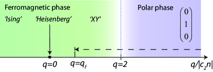
Figure 1: (Color Online) Zero-temperature phase diagram of a spin-1 Bose condensate indicating the transition from a polar phase to a ferromagnetic phase at low quadratic Zeeman energy (QZE). The dashed line indicates the direction of the quench from an initial QZE $q\gg 2|c_{2}|n_{0}$ to a final QZE $q=q_{f}$.

III Short-Time Theory

As illustrated in Fig. 1, for $q>q_{0}\equiv 2|c_{2}|n_{0}$, the ground state is the polar state while decreasing $q$ below $q_{0}$, the ground state acquires a magnetic moment and eventually reaches the fully polarized ferromagnetic state at $q=0$. Initially, we take $q=q_{i}$ to be the largest energy parameter in the Hamiltonian and quench to a final state $q=q_{f}$ where $0\leq q_{f}<q_{0}$. For short times, the dynamics is expected to be well-described by expanding the Hamiltonian to quadratic order around the initial polar state lamacraft07 ; saito07 ; damski07 ; uhlmann07 ; cherng08 ; baraban08 ; klempt09 , $\Psi=\sqrt{n_{0}}(0,1,0)^{T}$. Under this expansion the Hamiltonian becomes

$${\cal H} \approx\sum_{\bf k}\left((\varepsilon_{\bf k}+c_{2}n_{0}+q_{f})(\psi_{1,{\bf k}}^{\dagger}\psi_{1,{\bf k}}+\psi_{-1,{\bf k}}^{\dagger}\psi_{-1,{\bf k}})\right.$$

$$\qquad\left.+c_{2}n_{0}(\psi_{1,{\bf k}}^{\dagger}\psi_{-1,-{\bf k}}^{\dagger}+\psi_{-1,-{\bf k}}\psi_{1,{\bf k}})\right)$$ (4)

where we have dropped the term describing the stiff density fluctuations. For simplicity, we have considered the system in the continuum, in the absence of the trapping potential. In the ferromagnetic regime this quadratic Hamiltonian gives modes with imaginary frequencies, which correspond to unstable, exponentially growing in time modes lamacraft07 .

To quantify the spin dynamics after the quench, it is natural to consider transverse and longitudinal magnetization correlation functions

$$G_{\perp}({\bf r},t) =\frac{1}{n_{0}^{2}}\langle{:F_{+}({\bf r})F_{-}(0):}\rangle$$ (5)

$$G_{z}({\bf r},t) =\frac{1}{n_{0}^{2}}\langle{:F_{z}({\bf r})F_{z}(0):}\rangle$$ (6)

lamacraft07 and the concomitant gain functions, $G_{\perp}(t)$ and $G_{z}(t)$, which are the above evaluated for ${\bf r}=0$. For $q_{0}t/\hbar\gg 1$ and $q_{f}=0$, the above correlations within the linearized theory give

$$G_{\perp}(t) =\frac{1}{\sqrt{8\pi q_{0}t/\hbar}}\frac{1}{n_{0}\xi_{s}^{2}}e^{q_{0}t/\hbar}$$ (7)

$$G_{z}(t) =\frac{1}{64\pi q_{0}^{2}t^{2}\hbar^{2}}\frac{1}{(n_{0}\xi_{s}^{2})^{2}}e^{2q_{0}t/\hbar}$$ (8)

where $\xi_{s}=\sqrt{\hbar^{2}/q_{0}m}$ is the spin coherence length. Interestingly, the longitudinal gain grows with twice the exponent of the transverse gain. However, the longitudinal magnetization is suppressed by a large factor $1/(n_{0}\xi_{s}^{2})\sim 10^{-4}$ for the experimental parameters of Ref. sadler06 . Thus, $G_{z}(t)$ remains much smaller than $G_{\perp}(t)$ up to the times where the latter saturates $G_{\perp}(t)\approx 1$ and the linearized theory does not work (see Fig. 2).

IV Truncated Wigner Simulations

As seen from the exponential growth of the gain functions, the above theory clearly fails once the transverse magnetization is of order unity. To gain a more complete understanding we turn to truncated Wigner simulations. This technique involves propagating the full spinor Gross-Pitaevskii Equations (GPEs) of motion obtained by taking the classical limit of Eq. (1) seeded with random initial conditions for canonical degrees of freedom distributed according to the Wigner transform of the initial state. For our case the initial state is taken to be the vacuum of Bogoliubov quasiparticles for a theory expanded about the polar state. For the limiting case of $q_{i}=\infty$ this has the particularly simple form: $W({\Psi})\approx\delta(|\psi_{0,0}|^{2}-n_{0})\prod_{\bf k}8\exp\left[-2\sum_{\alpha}|\psi_{\alpha,{\bf k}}|^{2}\right],$ where the factor of $8$ ensures the correct normalization of the Wigner function polkovnikov10 .

To propagate the wave functions governed by the spinor GPE, we first discretize the system effectively by using a lattice with the constant $\ell$ chosen such that $\ell\ll\xi_{s}$ and $n_{0}\ell^{2}\gg 1$ and then use a split-operator method that is accurate up to cubic order in the time step size javanainen06 ; barnett10 . The TWA is an approximate method resulting in the leading order in the expansion of classical dynamics in quantum fluctuations polkovnikov10 . It is also known to be asymptotically accurate at short times and exact for quadratic theories. In our case we expect this method to be quantitatively accurate at all times. Indeed the small parameter of the expansion is $1/(n_{0}\xi_{s}^{2})\ll 1$ so that quantum corrections to TWA are suppressed by this factor and are potentially only important at very long times. At longer times when nonlinearities become relevant, the momentum modes become highly occupied and the dynamics remains classical. Putting the system on a lattice ensures that there is no potential spurious effect from vacuum occupation of high-energy modes, which sometimes impedes the validity of TWA at long times blakie08 . We checked that the results of our simulations are insensitive to the choice of the cutoff as long as it is shorter than the spin coherence length.

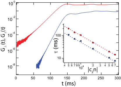
Figure 2: (Color Online) The growth of transverse (red) and longitudinal (blue) magnetization following a quench to $q_{f}=0$. Inset: The characteristic time constants for the growth of transverse and longitudinal magnetization densities versus the 2D interaction strength $|c_{2}n|$. The dashed lines indicate the predictions of the linearized Bogoliubov treatment for the respective parameters.

Shown in Fig. 2 are the TWA results for the transverse and longitudinal gain functions in the absence of a trap compared with the analytic results based upon the above linearized theory. At short evolution times following the quench, the simulations predict the exponential growth of both the transverse and longitudinal magnetization densities in a manner that is in excellent agreement with the linearized theory. During this period, the spin textures are characterized by ferromagnetic domains that are predominantly oriented in the transverse plane.

V Long-time behavior

We now move on to discuss the long-time dynamics of the quenched spinor condensate. As is seen in the gain functions in Fig. 2, the magnetization of the system eventually saturates and reaches a steady state. This motivates one to consider the prospect of thermalization in the system. More specifically, under the assumption of thermalization, the system will evolve to the ground state at $q=q_{f}$, with the excess energy accounted for by a superposition of elementary excitations about this configuration. We therefore will consider the theory about the state at $q=q_{f}$.

We define the heating (excess energy) of the system as

$$Q=\langle{\cal H}\rangle_{i}-\langle{\cal H}\rangle_{\rm gs}$$ (9)

where the above expectation values are evaluated for the initial state immediately after the quench and the ground state for $q=q_{f}$. To extract the equilibrium temperature this heating can be compared with the thermal energy of the system. It is convenient to use the following parameterization of the spinor

$$\Psi=\sqrt{n}e^{i\alpha}\left(\sin\eta\cos\phi e^{i\xi},\cos\eta e^{i\gamma},\sin\eta\sin\phi e^{-i\xi}\right)^{T}.$$ (10)

With this, one can see that for $0<q_{f}/q_{0}<1$ the classical energy is minimized for $\phi=\pi/4$, $\gamma=0$, and $\cos(2\eta)=q_{f}/q_{0}$. One then obtains that the above heating is

$$Q=\frac{1}{4}Nq_{0}\left(1-q_{f}/q_{0}\right)^{2}$$ (11)

where the details of this calculation are in Appendix A. Note that the above is based on classical energy differences. In addition to this classical contribution to the heating there is also a quantum correction coming from the zero point fluctuations of the condensate. However this contribution is suppressed by a large factor $\sqrt{n_{0}\xi_{s}^{2}}\sim 100$ and thus is not important.

The thermal energy of the final state is found from

$$Q=U(T)\equiv{\bf Tr}\left(e^{-{\cal H}/T}{\cal H}\right)/Z$$ (12)

where $Z={\bf Tr}\left(e^{-{\cal H}/T}\right)$ is the partition function and the ground state energy of the system is set to be zero. To evaluate the above we develop a second Bogoliubov theory by expanding the Hamiltonian to quadratic order about the minimum at $q=q_{f}$. Note that within the chosen parametrization one automatically avoids subtleties related to the lack of a long range order in two dimensions at finite temperatures. The quadratic theory is then self-consistently checked by verifying that the resulting thermal depletion is small for the computed temperature.

The full Bogoliubov analysis of the spectrum linearized around the ferromagnetic minimum is rather cumbersome because of the phonon-magnon coupling uchino10 (which vanishes for the special points $q_{f}=0$ and $q_{f}=q_{0}$). However, ⁸⁷Rb has a natural separation of energy scales since $c_{0}\gg|c_{2}|$ which inhibits density fluctuations. This significantly simplifies the Bogoliubov analysis and effectively results in the decoupling of the stiff density fluctuation and the spin modes. In this limit one finds the simplified spectrum consisting of two modes with the dispersion (see Appendix A)

$$\omega^{(\perp)}_{\bf k} =\sqrt{\varepsilon_{\bf k}(\varepsilon_{\bf k}+q_{f})}$$ (13)

$$\omega^{(z)}_{\bf k} =\sqrt{(\varepsilon_{\bf k}+q_{0})\left(\varepsilon_{\bf k}+\frac{q_{0}^{2}-q_{f}^{2}}{q_{0}}\right)}$$

where $\varepsilon_{\bf k}$ is the free particle dispersion. Note that these reduce to the known dispersions in the limits of $q_{f}=0$ and $q_{f}=q_{0}$ ho98 ; ohmi98 . Furthermore, the large $c_{0}$ limit of the full dispersion uchino10 agrees with Eq. (13). These expressions are used to compute the thermal energy of the system. It is straightforward to verify that unless $q_{f}$ is very close to $q_{0}$, $1-q_{f}/q_{0}\not\gg 1/\sqrt{n_{0}\xi_{s}^{2}}$, the dominant contribution to the thermal energy $U(T)$ comes from the quadratic dispersion of these modes: $\omega^{(\perp)}_{\bf k}\approx\omega^{(z)}_{\bf k}\approx\varepsilon_{\bf k}$. This can be justified a posteriori by comparing the temperature with $q_{0}$. With these conditions, $U(T)\approx N\pi T^{2}/6(n_{0}\xi_{s}^{2})q_{0}.$ Finally, equating this to the heating, one finds

$$T=\sqrt{\frac{3}{2\pi}n_{0}\xi_{s}^{2}}(q_{0}-q_{f}).$$ (14)

To test the hypothesis of thermalization, we use the developed quadratic theory to evaluate finite temperature correlation functions (evaluated at temperature Eq. (14)) and compare with long-time TWA results. The most natural correlation function to consider is $G_{\perp}$ defined in Eq. (5). The gapless mode, Eq. (13), which leads to algebraic decay of the correlation function in two dimensions has the dominant contribution. Within the quadratic Bogoliubov theory, the correlation function is found to be (see Appendix B)

$$G_{\perp}({\bf r})=\left[1-\left(q_{f}/q_{0}\right)^{2}\right](r/\xi_{s})^{-\alpha}$$ (15)

with exponent $\alpha=\sqrt{6/\pi^{3}}\cdot\sqrt{1/n_{0}\xi_{s}^{2}}$. Because of the dependence of the exponent $\alpha$ on the small parameter $1/n_{0}\xi_{s}^{2}$, we see that, assuming equilibrium, $G_{\perp}({\bf r})$ will not decay by any appreciable amount over the relevant length scales of the condensate, which are typically of the order of tens or hundreds of the spin coherence length $\xi_{s}$. For the same reason in equilibrium the system should not have any vortices.

We point out that the resulting thermal state of the condensate with temperature $T$ given by Eq. (14) has some interesting properties. On the one hand except for a small vicinity of $q_{f}\approx q_{0}$ it is a high-temperature classical state characterized by a temperature much higher than the chemical potential. This implies that quantum depletion in this state is negligible. On the other hand, the smallness of the exponent $\alpha$ shows that this state is well below the Kosterlitz-Thouless (KT) transition temperature due to the unbinding of vortices in the spin degrees of freedom. More specifically, the KT transition temperature scales as $T_{KT}\sim q_{0}n_{0}\xi_{s}^{2}$ which can be compared with Eq. (14). In this respect, this is a low-temperature state.

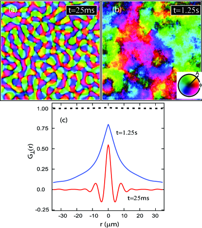
Figure 3: (Color Online) The transverse magnetization densities for short (a) and long (b) times for $q_{f}=0$ over a $70\times 70\mu{\rm m}$ region. The amplitude and orientation of the transverse magnetization are indicated by the brightness and hue (color wheel shown). (c) The spin correlation function for these same times. While the correlation function at short times is in excellent agreement with Bogoliubov theory, the decay of this function at long evolution times is much more rapid than predicted by Eq. (15) (dashed line).

We now compare these predictions to the results of the TWA simulations for long times. Shown in Fig. 3 are magnetizations for short and long times as well as correlation functions after the quench. Displayed are results for zero final quadratic Zeeman field $q_{f}=0$, though qualitatively very similar results occur for finite values of $q_{f}$ (for a full animation of the dynamics see EPAPS material barnett11 ). As shown in Fig. 3(c), the correlation function $G_{\perp}$ before saturation for short times has the functional dependence of a Bessel function $J_{0}(r/\xi_{s})$ as previously predicted lamacraft07 . For long times, the correlation function reaches a steady state and decays by over a factor of five from its $r=0$ value for a system size on the order of $50$ spin coherence lengths. Such decay is qualitatively incompatible with the theory developed by assuming thermalization. We thus conclude that these spinor condensate systems do not thermalize at appreciable time scales but rather reach a quasi-steady (prethermalized) regime which evolves anomalously slow in time. Such prethermalized phases were suggested earlier in the contexts of weakly interacting fermions moeckel_10 ; eckstein_kollar_09 , Bose superfluids mathey_10 ; kitagawa11 , and dynamics of the early Universe berges_borsanyi_04 . What is perhaps unexpected is that in this system anomalously slow relaxation occurs at very high levels of the heating in the system.

To support these results, it is useful to compare with the Landau damping rates of long-wavelength Bogoliubov modes as a result of scattering from thermal modes lifshitz81 ; pitaevskii97 ; giorgini98 ; pethick08 . Such an analysis is carried out in Appendix C. It is found that typical lifetimes of these modes is on the order of $100$ seconds. This rate is considerably lower than those of scalar condensates due to the weak spin-dependent interaction and small thermal depletion. The lifetime estimates provide lower bounds for the thermalization time and are consistent with the numerical results. However, such long time scales are outside of our numerical as well as experimental access.

In conclusion, we have examined the long time evolution of quantum degenerate spinor gases following a quench to a ferromagnetic phase. Assuming a thermalized final state, we find that the finite temperature spin correlations are characterized by an algebraic decay over length scales much larger than the relevant length scales of the condensate. In distinct contrast, numerical simulations based on the truncated Wigner approximation indicate a rapidly decaying correlation function even at extremely long evolution times. This inconsistency leads one to the conclusion that the quenched spinor condensates will not thermalize over experimentally relevant timescales. These results are consistent with the Landau damping rates. The role of dipolar interactions vengalatorre08 ; vengalattore10 in the long time evolution has yet to be examined.

Appendix A Bogoliubov analysis in the regime $0<q_{f}<2|c_{2}|n_{0}$

The easiest way to perform the Bogoliubov analysis of spinor condensates is to use a parametrization of the spinors though the density-angle variables as in Eq. (10). In this case one avoids issues related to absence of the true condensation in one-dimension at finite temperatures. Also the normal modes have a very transparent physical meaning. The analysis of this Appendix very closely mimics an analysis for the description of the low-energy excitations of bosons in an optical lattice close to the superfluid-insulator transition in the effective spin-one representation ehud_thesis ; altman_02 . In this parametrization, the magnetization $F_{z}=\Psi^{\star}f_{z}\Psi$ and $F_{z,2}=\Psi^{\star}f_{z}^{2}\Psi$ are given by

$$F_{z} = |\Psi_{1}|^{2}-|\Psi_{-1}|^{2}=n\sin^{2}(\eta)\;\cos(2\phi),$$ (16)

$$F_{z,2} = |\Psi_{1}|^{2}+|\Psi_{-1}|^{2}=n\sin^{2}(\eta).$$ (17)

Similarly the square of the transverse magnetization $|F_{\perp}|^{2}=F_{y}^{2}+F_{x}^{2}$ reads:

$$|F_{\perp}|^{2}={n^{2}\over 2}\sin^{2}(2\eta)[1+\sin(2\phi)\cos(2\gamma)].$$ (18)

With these expressions, one finds for the interaction energy density (here we include the quadratic Zeeman term in the interaction energy)

$$\mathcal{H}_{\rm int} = {c_{0}\over 2}n^{2}+{c_{2}\over 2}(F_{z}^{2}+|F_{\perp}|^{2})+qF_{z,2}$$ (19)

$$= {c_{0}\over 2}n^{2}+c_{2}n^{2}\sin^{2}(\eta)\cos^{2}(\eta)[1+\sin(2\phi)\cos(2\gamma)]$$

$$+ qn\sin^{2}(\eta)+{c_{2}n^{2}\over 2}\sin^{4}(\eta)\cos^{2}(2\phi).$$

It is straightforward to check that for $c_{2}<0$ and $0<q<2|c_{2}|n=q_{0}$ the energy is minimized when $\phi=\pi/4$, $\gamma=0$, and $\eta=\bar{\eta}$ where we define $\bar{\eta}$ according to $q=q_{0}\cos(2\bar{\eta})$. There is an equivalent minimum obtained by gauge transformation where $\phi\to\phi+\pi/2$ and $\gamma\to\gamma+\pi$. The minimum of the interaction energy density is then

$$E(q)\approx-q_{0}n\sin^{4}(\bar{\eta})=-{g_{0}n\over 4}\left(1-{q\over q_{0}}\right)^{2}.$$ (20)

Note that in this expression we ignored the zero point energy associated with the depletion, which is suppressed by a large factor $1/\sqrt{n_{0}\xi_{s}^{2}}$.

Within the Bogoliubov approximation we need to expand the energy around the minimum. For this purpose we define small deviations of the angles $\phi$ and $\eta$ from the optimal values $\phi=\pi/4+\delta\phi$, $\eta=\bar{\eta}+\delta\eta$ and do a second order expansion in $\delta\phi$, $\delta\eta$, $\gamma$, and $\xi$. Since we are interested in the limit $c_{0}\gg c_{2}$ the density fluctuations are suppressed and we can set $\delta n=0$ and fix the density at its equilibrium value $n=n_{0}$. Then the expression for the interaction energy density (19) reduces to

$$\delta\mathcal{H}_{\rm int}\approx q_{0}n_{0}\sin^{2}(\bar{\eta})$$

$$\times\left[\cos(2\bar{\eta})(\delta\phi)^{2}+\cos^{2}(\bar{\eta})\gamma^{2}+4\cos^{2}(\bar{\eta})(\delta\eta)^{2}\right].$$ (21)

Under the same approximation the kinetic energy density term reads

$$\mathcal{H}_{\rm kin}\approx{\hbar^{2}\over 2m}\biggl{[}(\nabla\delta\eta)^{2}+\sin^{2}(\bar{\eta})(\nabla\phi)^{2}+\sin^{2}(\bar{\eta})(\nabla\xi)^{2}$$

$$+\cos^{2}(\bar{\eta})(\nabla\gamma)^{2}+(\nabla\alpha)^{2}+2\nabla\alpha\nabla\gamma\cos^{2}(\bar{\eta})\biggr{]}.$$ (22)

And finally to determine the canonically conjugate variables we need to write the Berry phase term, $i\Psi^{\dagger}\dot{\Psi}$ in the linearized approximation:

$$2n_{0}\sin^{2}(\bar{\eta})\delta\phi\,\dot{\xi}+n_{0}\sin(2\bar{\eta})\delta\eta\,\dot{\gamma}-\delta n[\dot{\alpha}+\cos^{2}(\bar{\eta})\dot{\gamma}].$$ (23)

In this form it is clear that the phase conjugate to the density fluctuations is $\tilde{\alpha}=\alpha+\cos^{2}(\bar{\eta})\gamma$. Then the kinetic energy density can be rewritten as

$$\mathcal{H}_{kin}\approx{\hbar^{2}\over 2m}n_{0}\biggl{[}(\nabla\eta)^{2}+\sin^{2}(\bar{\eta})(\nabla\phi)^{2}+\sin^{2}(\bar{\eta})(\nabla\xi)^{2}$$

$$+(\nabla\tilde{\alpha})^{2}+\cos^{2}(\bar{\eta})\sin^{2}(\bar{\eta})(\nabla\gamma)^{2}\biggr{]}.$$ (24)

One can further redefine variables

$$\delta\phi\to\tilde{\phi}/(2\sqrt{n_{0}}\sin(\bar{\eta})),\quad\xi\to\tilde{\xi}/\sqrt{n_{0}}\sin(\bar{\eta}),$$

$$\gamma\to\tilde{\gamma}/\sqrt{n_{0}}\sin(2\bar{\eta}),\quad\eta\to\tilde{\eta}/\sqrt{n_{0}}.$$

Then, the spin part of the Lagrangian density (Berry phase minus Hamiltonian) becomes

$$\mathcal{L}\approx\tilde{\phi}\,\dot{\tilde{\xi}}+\tilde{\eta}\dot{\tilde{\gamma}}-g_{s}\left[{\cos(\bar{\eta}/2)\over 4}\tilde{\phi}^{2}+\cos^{2}\left({\bar{\eta}}\right)\tilde{\gamma}^{2}+\sin^{2}(2\bar{\eta})\tilde{\eta}^{2}\right]$$

$$-{\hbar^{2}\over 2m}\biggl{[}(\nabla\tilde{\eta})^{2}+{1\over 4}(\nabla\tilde{\phi})^{2}+(\nabla\tilde{\xi})^{2}+\cos^{2}\left({\bar{\eta}}\right)(\nabla\tilde{\gamma})^{2}\biggr{]}.$$ (25)

This Lagrangian density immediately gives two sets of normal modes corresponding to oscillations in the $\phi-\xi$ variables, which represent uniform rotations around $z$-axis, and in the $\eta-\gamma$ variables, which represent oscillations in the magnitude of the transverse magnetization. The corresponding frequencies in the momentum space are

$$\omega^{(\perp)}_{\bf k}=\sqrt{\varepsilon_{\bf k}(\varepsilon_{\bf k}+q_{0}\cos(2\bar{\eta}))},$$ (26)

$$\omega^{(z)}_{\bf k}=\sqrt{(g_{0}+\varepsilon_{\bf k})(\varepsilon_{\bf k}+q_{0}\sin^{2}(2\bar{\eta}))}$$ (27)

where $\varepsilon_{\bf k}=\frac{\hbar^{2}k^{2}}{2m}$ is the free particle dispersion. We note that these expressions follow from taking $c_{0}\to\infty$ limit of the general dispersion relations obtained in Ref. uchino10 . There are, however, advantages in using the density-angle representation since it does not rely on the assumption of the existence of the true long range order.

Appendix B Finite temperature correlation functions within the Bogoliubov theory

The Bogoliubov theory described in the previous section makes it possible to compute correlation functions in two-dimensional systems. In the following we will consider the transverse magnetization correlation function

$$G_{\perp}({\bf r},t) =\frac{1}{n_{0}^{2}}\langle{:F_{+}({\bf r})F_{-}(0):}\rangle.$$ (28)

Written in terms of the variables introduced in the previous section we have

$$F_{+}=\frac{1}{\sqrt{2}}ne^{i\alpha}\sin(2\eta)e^{-i\xi}\left(\cos(\phi)e^{i\gamma}+\sin(\phi)e^{-i\gamma}\right).$$ (29)

According to the Mermin-Wagner theorem, a gapless mode will lead to a power law behavior of correlation functions in two-dimensions. The gapless mode for our case corresponds to the $\phi-\xi$ variables. It is straightforward to see that these will dominate the correlation functions. Taking into account these two fluctuating fields one finds

$$<F_{+}({\bf r})F_{-}(0)>=\sin^{2}(2\bar{\eta})e^{-<\Delta\phi^{2}>/2}e^{-<\Delta\xi^{2}>/2}.$$ (30)

In this equation, $\langle{\Delta\xi^{2}}\rangle\equiv\langle{(\xi({\bf r})-\xi(0))^{2}}\rangle$ with a similar expression for $\langle{\Delta\phi^{2}}\rangle$.

Using the analysis from above, one finds

$$\langle{\Delta\xi^{2}}\rangle=\frac{1}{N\sin^{2}(\bar{\eta})}\sum_{{\bf k}}\frac{\omega_{\bf k}^{(\perp)}}{\varepsilon_{\bf k}}\left(f(\omega_{\bf k}^{(\perp)})+1/2\right)(1-J_{0}(kr)).$$ (31)

and

$$\langle{\Delta\phi^{2}}\rangle=\frac{1}{N\sin^{2}(\bar{\eta})}\sum_{\bf k}\frac{\varepsilon_{\bf k}}{\omega_{\bf k}^{(\perp)}}\left(f(\omega_{\bf k}^{(\perp)})+1/2\right)(1-J_{0}(kr))$$ (32)

where $f$ is the Bose distribution function. It can be seen that the dominant contribution comes from $\langle{\Delta\xi^{2}}\rangle$ due to the long-wavelength divergence of the sum over ${\bf k}$ which is cut off at $\sim 1/r$. The above expression is therefore well-approximated by

$$\langle{\Delta\xi^{2}}\rangle=\frac{T}{\pi\sin^{2}(\bar{\eta})q_{0}n_{0}\xi_{s}^{2}}\log(r/\xi_{s}).$$ (33)

Using the expression for the temperature derived in the manuscript, one arrives at Eq. (15).

Appendix C Landau Damping Rate

We take a spinor condensate with a single Bogoliubov excitation of wave vector ${\bf k}$ and evaluate its lifetime $\tau_{k}$ due to scattering off of short-wavelength thermal modes. For simplicity we will consider the gapless spin mode $\omega_{\bf k}^{\perp}$ as given in Eq. (13). Such a rate is given by the well-known Landau damping formula lifshitz81 which has been generalized to Bose-Einstein Condensates in pitaevskii97 ; giorgini98 ; pethick08

$$\frac{1}{\tau_{k}}=\frac{\pi}{\hbar}\sum_{\bf k^{\prime}}|M_{{\bf kk^{\prime}}}|^{2}(f(\omega_{\bf k}^{(\perp)})-f(\omega_{{\bf k}+{\bf k^{\prime}}}^{(\perp)}))\delta(\omega_{\bf k}^{(\perp)}+\omega_{\bf k^{\prime}}^{(\perp)}-\omega_{{\bf k}+{\bf k^{\prime}}}^{(\perp)}).$$ (34)

where $f$ is the Bose-Einstein distribution function. In this equation, the matrix element $M_{{\bf kk^{\prime}}}$ is given by pitaevskii97 ; giorgini98 ; pethick08

$$M_{{\bf kk^{\prime}}}=\frac{q_{f}}{2\sqrt{N}}\sqrt{\frac{\hbar k}{2ms}}\left(\frac{\varepsilon_{\bf k^{\prime}}}{\omega^{(\perp)}_{\bf k^{\prime}}}+\frac{\omega^{(\perp)}_{\bf k^{\prime}}}{\varepsilon_{\bf k^{\prime}}+q_{f}/2}\right)$$ (35)

where $s$ is the sound speed of the mode $\omega^{(\perp)}_{\bf k^{\prime}}$. With this expression, the two-dimensional ${\bf k^{\prime}}$-summation can be performed. In the limit $T\gg q_{f}$, the result is

$$\frac{1}{\tau_{k}}=\frac{a_{s}k}{\hbar}\frac{T}{d_{y}/\xi_{s}}\frac{q_{f}}{q_{0}}1.13=\frac{k\xi_{s}}{\hbar}\frac{T}{8\pi n_{0}\xi_{s}^{2}}\frac{q_{f}}{q_{0}}1.13$$ (36)

where $a_{s}=(a_{2}-a_{0})/3$ is the spin-dependent scattering length. Using the experimental parameters, and the expression for the temperature given in Eq. (14) and taking $q_{f}=q_{0}/2$ we find that

$$\tau_{k}\approx 90{\rm s}$$ (37)

for a mode having wave vector $q=1/(2\xi_{s})$.

References

- (1) L. E. Sadler, J. M. Higbie, S. R. Leslie, M. Vengalattore, and D. M. Stamper-Kurn, Nature 443, 312 (2006)
- (2) M. Vengalattore, S. Leslie, J. Guzman, and D. M. Stamper-Kurn, Phys. Rev. Lett. 100, 170403 (2008)
- (3) A. Lamacraft, Phys. Rev. Lett. 98, 160404 (2007)
- (4) H. Saito, Y. Kawaguchi, and M. Ueda, Phys. Rev. A 76, 043613 (2007)
- (5) B. Damski and W. H. Zurek, Phys. Rev. Lett. 99, 130402 (2007)
- (6) M. Uhlmann, R. Schützhold, and U. R. Fischer, Phys. Rev. Lett. 99, 120407 (2007)
- (7) R. W. Cherng, V. Gritsev, D. M. Stamper-Kurn, and E. Demler, Phys. Rev. Lett. 100, 180404 (2008)
- (8) M. Baraban, H. F. Song, S. M. Girvin, and L. I. Glazman, Phys. Rev. A 78, 033609 (2008)
- (9) C. Klempt, O. Topic, G. Gebreyesus, M. Scherer, T. Henninger, P. Hyllus, W. Ertmer, L. Santos, and J. J. Arlt, Phys. Rev. Lett. 103, 195302 (2009)
- (10) H. Saito, Y. Kawaguchi, and M. Ueda, Phys. Rev. A 75, 013621 (2007)
- (11) J. D. Sau, S. R. Leslie, D. M. Stamper-Kurn, and M. L. Cohen, Phys. Rev. A 80, 023622 (2009)
- (12) P. B. Blakie, A. S. Bradley, M. J. Davis, R. J. Ballagh, and C. W. Gardiner, Adv. in Phys. 57, 353 (2008)
- (13) A. Polkovnikov, Annals of Physics 325, 1790 (2010)
- (14) A. J. Bray, Adv. in Phys. 43, 357 (1994)
- (15) J. Javanainen and J. Ruostekoski, J. Phys. A 39, L179 (2006)
- (16) R. Barnett, E. Chen, and G. Refael, New J. Phys. 12, 043004 (2010)
- (17) S. Uchino, M. Kobayashi, and M. Ueda, Phys. Rev. A 81, 063632 (2010)
- (18) T.-L. Ho, Phys. Rev. Lett. 81, 742 (1998)
- (19) T. Ohmi and K. Machida, J. Phys. Soc. Japan 67, 1822 (1998)
- (20) R. Barnett, A. Polkovnikov, and M. Vengalattore (unpublished); See Supplemental Material at http://link.aps.org/supplemental/10.1103/PhysRevA.84.023606 for the full animation of the dynamics.
- (21) M. Moeckel and S. Kehrein, New J. of Phys. 12, 055016 (2010)
- (22) M. Eckstein, M. Kollar, and P. Werner, Phys. Rev. Lett. 103, 056403 (2009)
- (23) L. Mathey and A. Polkovnikov, Phys. Rev. A 81, 033605 (2010)
- (24) T. Kitagawa, A. Imambekov, J. Schmiedmayer, and E. Demler, arXiv:1104.5631
- (25) J. Berges, S. Borsányi, and C. Wetterich, Phys. Rev. Lett. 93, 142002 (2004)
- (26) E. M. Lifshitz and L. Pitaevskii, Physical Kinetics (Pergamon, Oxford, 1981)
- (27) L. Pitaevskii and S. Stringari, Phys. Lett. A 235, 298 (1997)
- (28) S. Giorgini, Phys. Rev. A 57, 2949 (1998)
- (29) C. J. Pethick and H. Smith, Bose-Einstein Condensation in Dilute Gases (Cambridge, 2008)
- (30) M. Vengalattore, J. Guzman, S. Leslie, F. Serwane, and D. Stamper-Kurn, Phys. Rev. A 81, 053612 (2010)
- (31) E. Altman, PhD thesis, Technion, 2002
- (32) E. Altman and A. Auerbach, Phys. Rev. Lett. 89, 250404 (2002)