Infrared Luminosities and Aromatic Features in the 24 $\mu$m Flux Limited Sample of 5MUSES

Abstract

We study a 24 $\mu$m selected sample of 330 galaxies observed with the Infrared Spectrograph for the 5 mJy Unbiased Spitzer Extragalactic Survey. We estimate accurate total infrared luminosities by combining mid-IR spectroscopy and mid-to-far infrared photometry, and by utilizing new empirical spectral templates from Spitzer data. The infrared luminosities of this sample range mostly from 10⁹L_⊙ to $10^{13.5}$L_⊙, with 83% in the range 10¹⁰L_⊙$<$L_IR$<$10¹²L_⊙. The redshifts range from 0.008 to 4.27, with a median of 0.144. The equivalent widths of the 6.2 $\mu$m aromatic feature have a bimodal distribution. We use the 6.2 $\mu$m PAH EW to classify our objects as SB-dominated (44%), SB-AGN composite (22%), and AGN-dominated (34%). The high EW objects (SB-dominated) tend to have steeper mid-IR to far-IR spectral slopes and lower L_IR and redshifts. The low EW objects (AGN-dominated) tend to have less steep spectral slopes and higher L_IR and redshifts. This dichotomy leads to a gross correlation between EW and slope, which does not hold within either group. AGN dominated sources tend to have lower log(L_PAH7.7μm/L_PAH11.3μm) ratios than star-forming galaxies, possibly due to preferential destruction of the smaller aromatics by the AGN. The log(L_PAH7.7μm/L_PAH11.3μm) ratios for star-forming galaxies are lower in our sample than the ratios measured from the nuclear spectra of nearby normal galaxies, most probably indicating a difference in the ionization state or grain size distribution between the nuclear regions and the entire galaxy. Finally, we provide a calibration relating the monochromatic 5.8, 8, 14 and 24 $\mu$m continuum or Aromatic Feature luminosity to L_IR for different types of objects.

1 Introduction

Infrared bright galaxies play critical roles in galaxy formation and evolution. The InfraRed Astronomical Satellite (IRAS) facilitated the study of an important group of objects, the Ultra Luminous InfraRed Galaxies (ULIRGs) (Soifer et al., 1989; Sanders & Mirabel, 1996), which were first hinted at by ground based observations of Rieke & Low (1972). Studies from the Infrared Space Observatory (ISO) (Elbaz et al., 1999) and the Spitzer Space Telescope (Houck et al., 2005; Yan et al., 2007) later revealed that LIRGs and ULIRGs are much more common at high redshift than in the local Universe. The number density of IR luminous galaxies evolves strongly with redshift to at least z$\sim$1 (Le Floc’h et al., 2005). The fraction of galaxies powered by star formation versus AGN is still controversial, but is crucial for determining unbiased luminosity functions for various categories of objects and understanding the evolution process.

The superb sensitivity of the Spitzer Space Telescope (Werner et al., 2004) has led to the discovery of new populations of faint, high-redshift galaxies with extreme IR/optical colors (Dickinson et al., 2004; Houck et al., 2005; Weedman et al., 2006; Yan et al., 2007; Caputi et al., 2007; Dey et al., 2008; Dasyra et al., 2009). However, these studies often have at least one other constraint than the mid-IR flux limit, usually a minimum R band magnitude or an IRAC-based color selection, designed to favor sources in specific redshift ranges, or with high luminosity. The 5 Millijanksy Unbiased Spitzer Extragalactic Survey (5MUSES) is an infrared selected sample. A major advantage of 5MUSES is its simple selection: f_ν(24$\mu$m)$>$5mJy. This relatively bright flux limit allows for a more detailed study of the infrared properties, filling in the gap between local galaxies and high redshift samples, and helping to improve the modeling of galaxy populations and their evolution.

In order to advance our understanding of the properties and evolution of galaxies, it is crucial to obtain accurate estimates of their bolometric luminosities. Several studies have shown that monochromatic luminosities in the mid-IR can be used to estimate L_IR (Sajina et al., 2007; Bavouzet et al., 2008; Rieke et al., 2009; Calzetti et al., 2010), and the uncertainties on these estimates decrease significantly when far-infrared (FIR) fluxes are available (Kartaltepe et al., 2010). However, the spectral energy distribution (SED) of star-forming galaxies, AGN and ULIRGs display a wide range of shapes (Weedman et al., 2005; Brandl et al., 2006; Smith et al., 2007; Armus et al., 2007; Hao et al., 2007; Wu et al., 2009; Veilleux et al., 2009). Applying these methods without knowing a source’s spectral type could cause significant biases in luminosity estimates between types of objects and seriously mislead the interpretations. The 5 to 36 $\mu$m spectra obtained by the Infrared Spectrograph (IRS) (Houck et al., 2004) for the 5MUSES sample allows for aromatic feature identification, excitation line analysis, and decomposition into star formation and AGN components, thus providing essential information for classifying the origin of the luminosity.

The mid-IR is home to a set of broad emission line features, which are thought to originate from Polycyclic Aromatic Hydrocarbons (Puget et al., 1985; Allamandola et al., 1989). PAHs are organic molecules that are ubiquitous in our own Galaxy (Peeters et al., 2002) and nearby star-forming galaxies (Helou et al., 2001; Smith et al., 2007). In total, they can contribute a significant fraction (10% or more) of the total infrared luminosity in star-forming galaxies. PAHs are weak in low metallicity galaxies (Madden et al., 2006; Wu et al., 2006; Engelbracht et al., 2008), or in galaxies with powerful (Roche et al., 1991; Weedman et al., 2005; Armus et al., 2007; Desai et al., 2007; Wu et al., 2009) or even weak AGN (Smith et al., 2007; Dale et al., 2009). The PAH features, including their profiles, central wavelengths and band-to-band intensity ratios have been studied in detail by Peeters et al. (2002), Smith et al. (2007) and most recently reviewed by Tielens (2008). The 6.2 $\mu$m feature and the 7.7 $\mu$m complex are attributed to vibrational modes of the carbon skeleton. The 8.6 $\mu$m feature is attributed to in-plane C-H bending, while the features at 11.3 $\mu$m and 12.7 $\mu$m are identified as out-of-plane C-H bending modes. It is generally thought that charged PAHs radiate more strongly in the C-C vibrational modes, while neutral PAHs radiate strongly in the out-of-plane C-H bending modes at 11.3 $\mu$m and 12.7 $\mu$m. The fraction of the power radiated by PAH in the different bands following single-photon heating depends on both the PAH ionization and on the size of the PAH (Draine & Li, 2007). Thus the observed variations in the PAH band-to-band ratios can reflect variations in physical conditions (Smith et al., 2007; Galliano et al., 2008; Gordon et al., 2008; O’Dowd et al., 2009).

Because PAH emission can be very prominent in star-forming systems, it has often been used as a relatively extinction-free diagnostic tool to constrain star formation. Detailed studies on the properties of PAH features locally (Spoon et al., 2007; Desai et al., 2007) and at higher redshift (Yan et al., 2005; Houck et al., 2005; Huang et al., 2009) reveal differences in the PAH Equivalength Widths (EWs) and L_PAH/L_IR ratios. This might indicate that some evolution in the PAH properties occurs with redshift, or that sample selection effects make for large variations in the aromatic feature properties. However, one cannot simply apply our knowledge from the local universe to high redshift galaxies, or make fair comparisons between the two unless truly equivalent samples have been studied. Current analysis on the PAH properties are based on ISO or Spitzer observations of relatively bright objects, which have been selected because of previously known optical or IRAS criteria. Thus it is crucial to have a complete or at least unbiased census of galaxies in order to understand the galaxy evolution process and its relation to the aromatic feature emission.

In this paper, we study the properties of PAH emission and IR luminosities. This is the first of a series of papers to study the IR selected representative sample of 5MUSES. Helou et al. (in preparation) will address the general properties of the sample and how it bridges the gap between local and high-z galaxies. Yong et al. (in preparation) will present the correlations between old stars and current star formation. Detailed population modelling will also be performed to address the bimodal distribution of the PAH EWs discovered in this study. In Section 2, we briefly describe the sample selection, data reduction and measurements of spectral features. We introduce our library of empirical IR SED templates built upon Spitzer observations in Section 3, and derive the total infrared luminosities for 5MUSES galaxies. We also discuss how well one can constrain the IR SED if only mid-IR data are available. In Section 4, we study the properties of PAH emission from our flux limited sample. Finally, we present our conclusions in Section 5. Using the IR luminosities we derived in Section 3 and the PAH luminosities from Section 4, we discuss estimation of L_IR from PAH luminosity or monochromatic continuum luminosity in the Appendix. Throughout this work, we assume a $\Lambda$CDM cosmology with H₀=70 km s^-1 Mpc^-1, $\Omega_{m}$=0.27 and $\Omega_{\lambda}$=0.73.

2 Observations and Data Analysis

2.1 The Sample

5MUSES is a mid-IR spectroscopic survey of a 24 $\mu$m flux-limited (f${}_{24\mu m}>$5 mJy) representative sample of 330 galaxies. The galaxies are selected from the SWIRE fields (Lonsdale et al., 2003), including Elais-N1 (9.5 deg²), Elais-N2 (5.3 deg²), Lockman Hole (11.6 deg²) and XMM (9.2 deg²), in addition to the Spitzer Extragalactic First Look Survey (XFLS, 5.0 deg²) field (Fadda et al., 2006). It provides a representative sample at intermediate redshift ($<z>\sim$0.144) which bridges the gap between the bright, nearby star-forming galaxies (Kennicutt et al., 2003; Smith et al., 2007; Dale et al., 2009), local ULIRGs (Armus et al., 2007; Desai et al., 2007; Veilleux et al., 2009) and the much fainter and more distant sources pursued in most z$\sim$2 IRS follow-up work to date (Houck et al., 2005; Yan et al., 2007). The full details of the sample, including selection criteria and observation strategy are covered in Helou et al. (2010, in prep).

2.2 Observation and Data Reduction

Because of its selection in the SWIRE and XFLS fields, IRAC 3.6-8.0 $\mu$m photometry is available for the entire 5MUSES sample. In addition to the MIPS 24 $\mu$m photometry used to select this sample, 90% of our sources have also been detected at MIPS 70 $\mu$m and 54% have been detected at MIPS 160 $\mu$m. Low-resolution spectra (R=64$\sim$128) of all 330 galaxies in 5MUSES have been obtained with the Short-Low (SL: 5.5-14.5 $\mu$m and Long-Low (LL: 14-35 $\mu$m) modules of the IRS using the staring mode observations. The integration time on each object was estimated based on its 24 $\mu$m flux densities and typically ranges from 300-960 seconds (see Table 1). A sub-set of the 5MUSES sample has also been observed with the high-resolution modules of the IRS, which will be covered in a future paper.

The low-resolution IRS data were processed by the Spitzer Science Center data reduction pipeline version S17. The two-dimensional image data were converted to slopes after linearization correction, subtraction of darks, cosmic-ray removal, stray light and flat field correction. The post-pipeline reduction of the spectral data started from the pipeline products basic calibrated data (bcd) files. We took the median of all images from the off-source part of the slit (off-order and off-nod) and then subtracted it from the image on the source. Then we combined all the background-subtracted images at one nod position and took the mean. The resulting images were then cleaned with the IRSCLEAN package to remove bad pixels and apply rogue pixel correction.

We used the Spitzer IRS Custom Extractor (SPICE) software to extract the spectra. With a flux limit of 5 mJy at 24 $\mu$m, we chose to use the optimal extraction with point-source calibration because it significantly improved the S/N ratios for our sources. When using the optimal method, each pixel was weighted by its position, based on the spatial profile of a bright calibration star. The outputs from SPICE produced one spectrum per order at each nod position, which were then combined. We also trimmed the ends of each order where the noise rose quickly. Finally, the flux-calibrated spectra of each order (including the 1st, 2nd and 3rd orders) and module were merged without applying any scaling factor between SL and LL, and yielded a single spectrum per source. This spectrum was used to estimate aromatic feature fluxes, continuum flux densities at various wavelengths and line fluxes.

2.3 Data Analysis

2.3.1 The PAH Fluxes and Equivalent Widths

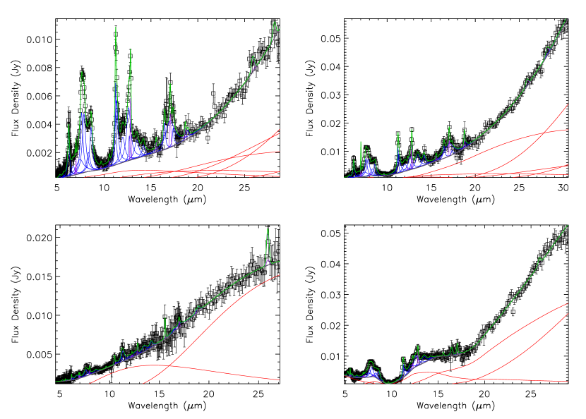
Figure 1: Examples of PAHFIT decomposition of 5MUSES spectra (black squares) with strong, moderate, weak PAH emission and with silicate absorption. The best fit SED (green) is composed of thermal dust continua (red), PAH features (blue), stellar light (magenta) and emission lines (purple).

To study the properties of PAH emission in our sample, we have used two methods to estimate the feature strength. The first method defines a local continuum or “plateau” under the emission features at 6.2 and 11.3 $\mu$m by fitting a spline function to selected points, and measures the features above the continuum. The wavelength limits for the integration of the features are approximately 5.95-6.55 $\mu$m for the 6.2 $\mu$m PAH and 10.80-11.80 for the 11.3 $\mu$m PAH. We have not taken into account the possibility of water ice or HAC absorption in our measurement of the 6.2 $\mu$m PAH EW because these features are known to be important mainly in strongly obscured local ULIRGs (Spoon et al., 2004); thus neglecting this component does not significantly change the 6.2 $\mu$m PAH EW. Although the 9.7 $\mu$m silicate feature could affect the measurement on the 11.3 $\mu$m PAH, our sample has very few deeply obscured sources. The PAH EWs are derived by dividing the integrated flux over the average continuum flux in each feature range. This PAH EW measured from the spline fitting method is defined as the “apparent PAH EW” and is directly comparable to the studies in the literature such as Peeters et al. (2002); Spoon et al. (2007); Armus et al. (2007); Desai et al. (2007); Pope et al. (2008) and Dale et al. (2009). In the second method, we use the PAHFIT software (Smith et al., 2007) to measure the PAHs in our sample (see Figure 1 for examples). In PAHFIT, the PAH features are fit with Drude profiles, which have extended wings that account for a significant fraction of the underlying plateau (Smith et al., 2007). As has been shown in Smith et al. (2007) and Galliano et al. (2008), although the PAHFIT method gives higher values of PAH integrated fluxes or EWs due to the lower continuum adopted than the “apparent PAH EW” method, the two methods yield consistent results on trends, such as the variations of band-to-band PAH luminosity ratios. Throughout this paper, when we refer to PAH EWs, we mean the apparent PAH EWs measured from the spline fitting method and they are used to classify object types. When we refer to PAH flux or luminosity, we mean the values derived from PAHFIT.

2.3.2 The Fine-Structure Line Fluxes

The mid-IR has a rich suite of fine-structure lines. [SIV]10.51$\mu$m, [NeII]12.81$\mu$m, [NeIII]15.55$\mu$m, [SIII]18.71/33.48$\mu$m and [SiII]34.82$\mu$m are the most frequently detected fine-structure lines in the spectral range covered by the IRS. The high-excitation line of [OIV]25.89$\mu$m has often been detected in low metallicity galaxies, starburst galaxies or AGN, excited by the photoionization and/or shocks associated with intense star formation or nuclear activity, while the [NeV]14.32/24.32$\mu$m lines are frequently detected in AGN-dominated sources and serve as unambiguous indicators of an AGN.

We use the ISAP package in SMART (Higdon et al., 2004) to measure the strength of the fine-structure lines. A Gaussian profile is adopted to fit the lines above a local continuum. The continuum is derived by linear fitting except for the [NeII]12.81$\mu$m line, which is blended with the 12.7 $\mu$m PAH feature. The continuum underlying the [NeII] line is fit with a 2nd-order polynomial. The integrated fitted flux above the continuum is taken as the total flux of the line. Upper limits are derived by measuring the flux with a height of three times the local rms and a width equal to the instrument resolution. In this paper, we only use the flux ratio of [NeIII]/[NeII] to compare with the PAH strength, while the tabulated line fluxes will be presented and discussed in a future paper.

3 The Infrared Luminosities of the 5MUSES Sample

Several SED libraries have been built to capture the variation in the shape of IR SEDs and to estimate L_IR (Dale & Helou, 2002; Chary & Elbaz, 2001; Draine & Li, 2007; Rieke et al., 2009). In the absence of multi-wavelength data, monochromatic luminosities have also been widely used to estimate L_IR (Sajina et al., 2007; Bavouzet et al., 2008; Rieke et al., 2009; Kartaltepe et al., 2010). The 5MUSES sample has mid-IR spectra, in addition to the IRAC and MIPS photometry, which allows us to account properly for variations in the SED shape and obtain more accurate estimates of L_IR.

3.1 Constructing an SED Template Library

In order to cover a wide range of SED shapes to fit the 5MUSES sources, we have built an IR template library based on the recent observations obtained from Spitzer. The library encompasses 83 ULIRGs observed by the IRS GTO sample (Armus et al., 2007); 75 normal star-forming galaxies from Spitzer Infrared Nearby Galaxies Survey (SINGS, Kennicutt et al. (2003)); and 136 PG and 2MASS quasars (Shi et al., 2007). The templates in the library consist of SEDs derived from IRS spectra and/or IRAC and MIPS photometry. For both the ULIRG and PG/2MASS sources, full 1-1000 $\mu$m SED have been obtained by Marshall et al. (2010, in preparation) and Shi et al.(2010, in preparation) from IRS, MIPS and IRAS observations. For the SINGS galaxies, Dale et al. (2007) have provided SED fits to the MIPS 24, 70 and 160 $\mu$m photometry using the Dale & Helou (2002) templates. However, these templates do not sample the full variation of the strength of PAH features in the 5-15 $\mu$m regime, due to the limited mid-IR spectra available when the templates were created. As a result, when we use SINGS galaxies as templates, we use their FIR SED from the fits of Dale et al. (2007), while in the mid-IR, we use the observed IRAC photometry integrated from the whole galaxy. This extensive template library provides a good coverage on the variations of IR SEDs. 33% of our sources are best-fit with SINGS-type templates and 38% are best-fit with quasar-type templates. The remaining sources are best-fit by ULIRG-type templates. The type of the best-fit template also correlates well with the 6.2 $\mu$m PAH EWs. SB-dominated sources are normally best fit by SINGS-type templates and AGN-dominated sources are best-fit with quasar-type templates. For SB-AGN composite sources, the best-fit templates are divided among ULIRG, SINGS and quasar-type templates (48%, 37% and 15% respectively).

3.2 Estimating L_IR using Spitzer data

Out of the 330 sources in 5MUSES, 280 galaxies have redshifts from optical or mid-IR spectroscopy. We are in the process of obtaining spec-z for the remaining 50 sources. We have estimated redshifts for 11 out of these 50 objects from silicate features or very weak PAH features, but do not include them in the discussion of this paper because of the large associated uncertainties. For the 280 objects, we use a combination of synthetic IRAC photometry obtained from the rest-frame IRS spectra, as well as the observed MIPS photometry to compare with the corresponding synthetic photometry from the SED templates and estimate total L_IR. We select the best-fit template by minimizing $\chi^{2}$ and we use progressively more detailed and accurate L_IR estimation methods for 5MUSES source with more photometry available. The final SED is composed of the IRS spectrum in the mid-IR and the best-fit template SED in the FIR. In the remainder of this section, we describe our method for estimating L_IR and the associated uncertainties.

3.2.1 Sources with MIPS FIR photometry

For sources with FIR detection at MIPS 70 and 160 $\mu$m, we use five data points to fit their SEDs. The first two data points are rest-frame IRAC 5.8 and 8.0 $\mu$m derived by convolving the rest-frame 5MUSES spectrum with the filter response curves of IRAC 5.8 and 8.0 $\mu$m. The other three data points are the observed MIPS 24, 70 and 160 $\mu$m photometry for each 5MUSES source. The corresponding data points from the templates are derived in the following way: For ULIRG and PG/2MASS templates, the 5.8 and 8.0 $\mu$m fluxes are derived in the same manner as 5MUSES sources. The 24, 70 and 160 $\mu$m data points are derived by convolving the template SED at matching redshift with the MIPS 24, 70 and 160 $\mu$m filter response curves. For SINGS templates, we use directly the observed IRAC 5.8 and 8.0 $\mu$m photometry as the first two data points, which are essentially at rest-frame for all SINGS objects. Then we move the SINGS SEDs given by Dale et al. (2007) to the redshift of the 5MUSES source and derive the corresponding observed-frame MIPS 24, 70 and 160 $\mu$m photometry. During the SED fitting, we weight the data points by their wavelength since the majority of the energy is emitted at FIR for IR selected sources, and look for the template that fits each 5MUSES source best by minimizing the $\chi^{2}$. A comparison of the ratio of flux densities at rest-frame 5.8, 8.0 $\mu$m and the observed MIPS 24, 70 and 160 $\mu$m photometry from the source and the best-fit template can be found in Figure 2 (solid line). The dispersion in the ratio of the observed photometry over the photometry from the best-fit template (F_source/F_template) in each band is 0.07, 0.07, 0.03, 0.06 and 0.10 dex respectively.

For sources with FIR detection only at MIPS 70 $\mu$m, we apply the same technique to fit the SED. We use the rest-frame IRAC 5.8 and 8.0 $\mu$m photometry and the observed MIPS 24 and 70 $\mu$m data in our fitting. The upper limit at 160 $\mu$m is used to exclude templates for which the synthetic photometry exceeds the 2$\sigma$ upper limit of the source. A comparison of the ratio of flux densities at rest-frame 5.8, 8.0 $\mu$m and the observed MIPS 24 and 70 $\mu$m photometry from the source and the best-fit template can be found in Figure 2 (dashed line). The dispersion in the ratio of F_source/F_template in each band is 0.07, 0.07, 0.03 and 0.07 dex respectively.

Once the best-fit template is identified, we derive L_IR as explained in the last paragraph of the next section.

3.2.2 Sources without MIPS FIR photometry

19 objects do not have FIR detection even at 70 $\mu$m. For these sources, we select the IR SED based on the mid-IR spectra. Our method is to fit the IRS spectrum of the 5MUSES source with the mid-IR spectra of the templates in the corresponding wavelength regime and adopt the SED of the best-fit template. The templates of which the synthetic photometry exceed the 2$\sigma$ upper limits at MIPS 70 and 160 $\mu$m bands are excluded. As will be shown in Section 3.2.3, this IRS-only method might underestimate the L_IR for cold sources by $\sim$20%, while it shows no significant offset for warm sources. All of the 19 objects in this category show SEDs with high ($f_{\rm 24\mu m}/f_{\rm 70\mu m}$)_obs ratios; thus they are more likely to be warm sources. This suggests that our approach of using the IRS spectrum to find the best-fit SED is unlikely to result in significant biases on L_IR.

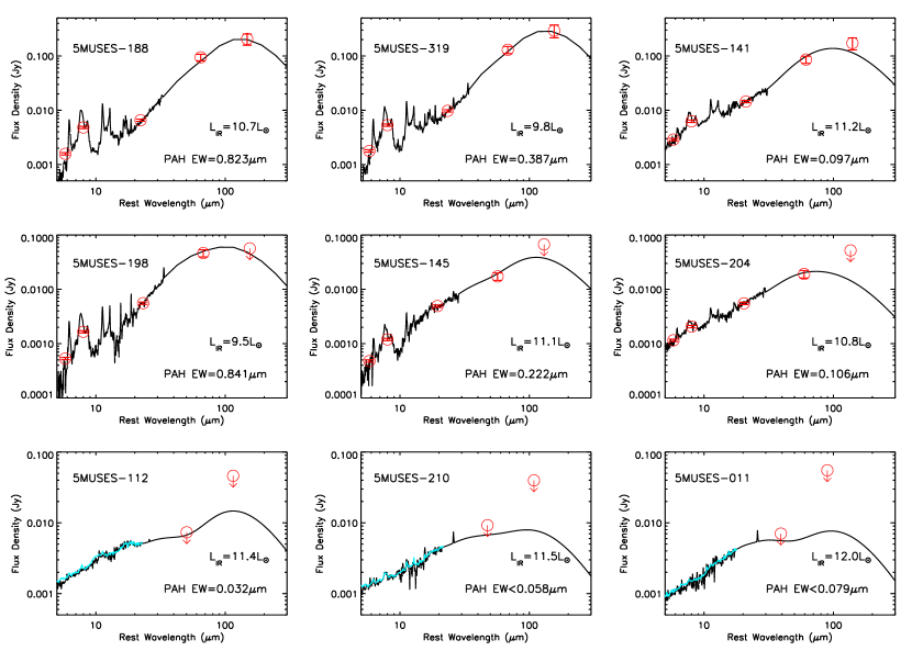
Figure 3: SEDs of a sample of nine 5MUSES sources. The final SED (black) is composed of the IRS spectrum in the mid-IR and the best-fit template in the FIR. The observed data are shown as red circles. The three sources in the top panel are fit with 5 data points (IRAC 5.8, 8.0 $\mu$m and MIPS 24, 70 and 160 $\mu$m). The three sources in the middle panel are fit with 4 data points (IRAC 5.8, 8.0 $\mu$m and MIPS 24 and 70 $\mu$m). The three sources in the bottom panel are fit with only the IRS spectra. The blue line is the mid-IR SED of the best-fit template for the sources fit with the IRS spectra.

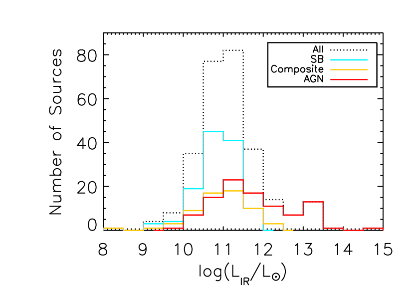
Figure 4: a) Top panel: The distribution of the total infrared luminosity of the 5MUSES sample. The dotted line represents the whole sample with known redshift. The blue, yellow and red solid lines represent the SB, composite and AGN sources in the sample. The SBs and AGN dominate the lower and higher end of the luminosity distribution respectively. b) Bottom panel: The distribution of the redshifts of the 5MUSES sample. The symbols are the same as in a).

Finally, for each source, we visually inspect the fitting results. We find that a range of templates could fit the SED well. We construct the final 5-1000 $\mu$m SED of a galaxy by combining its IRS spectrum in the mid-IR with the best-fit template SED at FIR. The total IR luminosity is derived by integrating under this SED curve. The uncertainty is derived from the standard deviation among the six best fits. We show examples of our SED fitting results in Figure 3 and the distribution of L_IR is shown Figure 4 a . We also show the distribution of L_IR for each type of objects, e.g. starburst, AGN and composite (defined in detail in Section 4.1) in this figure. The derived L_IR for each source and its uncertainty is tabulated in Table 2. The distribution for the redshifts of 5MUSES objects are shown in Figure 4 b.

3.2.3 How well can we constrain IR SED from mid-IR?

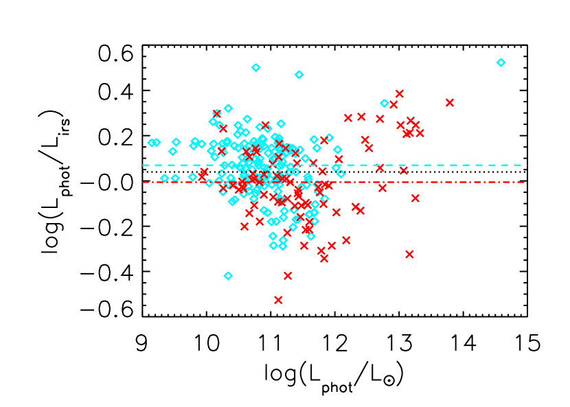
Figure 5: The ratio of the L_IR derived from using IRAC 5.8, 8.0 and MIPS 24, 70 and 160 $\mu$m photometry over L_IR predicted by IRS spectra versus L_IR. The diamonds represent cold sources with $f_{\rm 24\mu m}/f_{\rm 70\mu m}<$0.2 and the crosses represent the warm sources with $f_{\rm 24\mu m}/f_{\rm 70\mu m}>$0.2. The dotted line indicate the median of the luminosity ratios ($L_{\rm phot}/L_{\rm IR}=$1.10, 1$\sigma$=0.16 dex). The dashed line indicates the median ratio for the cold sources ($L_{\rm phot}/L_{\rm IR}=$1.17, 1$\sigma$=0.14 dex) and the dot-dashed line indicates the median ratio for the warm sources ($L_{\rm phot}/L_{\rm IR}=$0.99, 1$\sigma$=0.18 dex).

As has been shown above as well as in Kartaltepe et al. (2010), the availability of longer wavelength data greatly reduces the uncertainty in the estimate of L_IR. We need to quantify how well one can constrain the SED of a galaxy if only the continuum shape up to $\sim$30 $\mu$m is available. In Figure 5, we show the comparison of the IRS predicted L${}_{\rm IR}^{\rm IRS}$ and the L${}_{\rm IR}^{\rm phot}$ estimated from photometric data points (IRAC 5.8, 8.0 $\mu$m and MIPS 24, 70 and 160 $\mu$m). For the IRS-only method, we use only the IRS spectrum and do not employ any longer wavelength information (70 and 160 $\mu$m fluxes or upper limits) in our SED fitting, with the goal of testing solely the power of using mid-IR SED to predict FIR SED. We find that L_IR estimated from mid-to-FIR photometry are on average 10% higher than L_IR estimated from the IRS-only method, with a considerable scatter of 0.14 dex. It is worth noting that L${}_{\rm IR}^{\rm IRS}$ deviates from L${}_{\rm IR}^{\rm phot}$ by more than 0.2 dex for 20% of the sources while 5% of the sources deviate by more than 0.3 dex. We further divide the sources into two groups: cold sources and warm sources, based on the ratio of $f_{\rm 24\mu m}/f_{\rm 70\mu m}$. Cold sources ($f_{\rm 24\mu m}/f_{\rm 70\mu m}<$0.2) show an average underestimate of 17% when using the IRS-only method and the 1$\sigma$ scatter is 0.16 dex, while warm sources ($f_{\rm 24\mu m}/f_{\rm 70\mu m}>$0.2) do not show systematic offset in the estimated L_IR from the two methods, with a scatter of 0.18 dex. This comparison suggest that in IR-selected samples, the mid-IR spectrum could be used as an important indicator for L_IR when no longer wavelength data are available. However, for cold sources, the IRS-only method might underestimate L_IR by $\sim$17%, due to the lack of information on the peak of the SED. For warm sources, although L_IR estimated from the IRS-only method generally agrees with the value estimated from mid-to-far IR SED, the associated uncertainty is rather large. Thus for an individual galaxy, the L_IR predicted by its mid-IR SED could be a factor of 1.5 off from its intrinsic value for a significant subset of the population.

3.3 Estimating the total IR Luminosity from a Single Band

Using Spitzer data, we have obtained accurate estimates of the total infrared luminosities for 5MUSES. In the absence of multi-wavelength data, single-band luminosities have often been used to estimate L_IR (Sajina et al., 2007; Papovich et al., 2007; Pope et al., 2008; Rieke et al., 2009; Bavouzet et al., 2008; Symeonidis et al., 2008). However, the fractional contribution of these photometric bands to the total infrared luminosity varies substantially depending on the dominant energy source. Because the IRS spectrum provides an unambiguous way to identify the energy source for 5MUSES galaxies, our sample is ideal for investigating the difference in the fractional contributions of single band luminosities to L_IR in different types of objects.

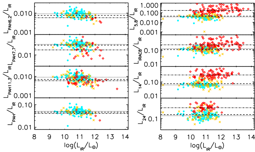
Figure 6: The luminosity ratio of several bands over L_IR versus L_IR. The blue circles, yellow crosses and red diamonds represent the SB, composite and AGN dominated sources in 5MUSES. The dotted, dash, and dash-dotted lines stand for the median ratios for the SB, composite and AGN sources, respectively. The PAH luminosities are derived from PAHFIT measurements. The 5.8, 14 and 24 $\mu$m luminosities are monochromatic luminosities calculated from the continua at these wavelengths. The IRAC 8 $\mu$m luminosities are derived by convolving the rest-frame IRS spectra with the filter response curve of the IRAC 8 $\mu$m band. The ratios and the associated uncertainties are also listed in Table 3.

In Figure 6, we plot the ratio of several luminosity bands to L_IR. The PAH luminosities are plotted on the left panel and continuum luminosities are on the right. The dotted, dashed and dash-dotted lines respectively stand for the median ratios for SB, composite and AGN dominated sources. Clearly the fractional contribution of a certain band to L_IR is highly dependent on the type of the object, e.g. the monochromatic 24 $\mu$m continuum luminosity $\nu$L_ν accounts for $\sim$13% of the total IR luminosity for SB galaxies, while it can contribute on average 30% of L_IR in AGN. The difference in the ratio of PAH luminosity to L_IR is less significant for different types of objects, because in order to be included on the left panel of this plot, the AGN dominated sources also need to have a solid detection of PAH feature that could be measured by PAHFIT, i.e. strong AGN sources are excluded. The mean ratios of L_singleband/L_IR are summarized in Table 3. Finally, we also provide our calibration of using single band luminosity to estimate L_IR in the Appendix.

4 Aromatic Feature Diagnostics

4.1 The Average Spectra

We derive the stacked SEDs for the SB, composite and AGN dominated sources in the 5MUSES sample, combining the low resolution IRS spectra in the mid-IR with the MIPS photometry at FIR. Although we do not have optical spectroscopy to classify the object types with the BPT diagram (Baldwin et al., 1981; Kewley et al., 2001), the equivalent widths of PAH features can be used as indicators of star formation activity. The 6.2 and 11.3 $\mu$m PAH bands are relatively isolated with little contamination from nearby features, which is important for unambiguously defining the local continuum. However, the 11.3 $\mu$m band is located on the shoulder of 9.7 $\mu$m silicate feature. Thus its integrated flux and underlying continuum are likely to be affected by dust extinction effects. As a result, in our discussion, we use the 6.2 $\mu$m PAH EWs to classify objects. To be consistent with the studies in the literature, we have adopted the following criteria for our spectral classification: sources with EW$>$0.5 $\mu$m are SB-dominated; sources with 0.2$<$EW$\leq$0.5 $\mu$m are AGN-SB composite and sources with EWs$\leq$0.2 $\mu$m are AGN-dominated. (Armus et al., 2007). The PAH EWs for the sample are tabulated in Table 2. Out of the 280 sources for which redshifts have been obtained from optical or infrared spectroscopy, there are 123 SB galaxies (44%), 62 composite sources (22%) and 95 AGN dominated sources (34%).

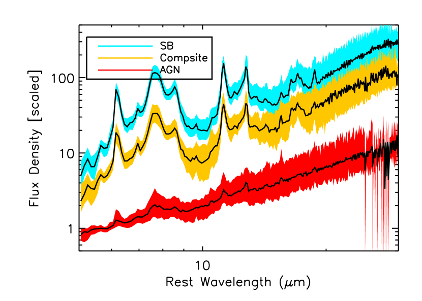
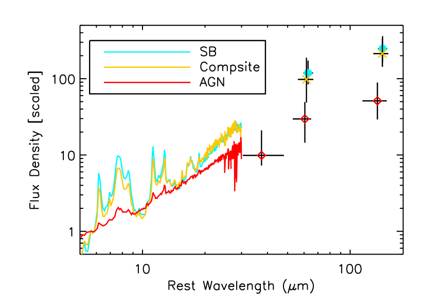
Figure 7: a) Left panel: The median IRS spectra for SB, composite and AGN dominated sources from 5MUSES after normalizing at 5.8 $\mu$m. The SEDs have been offset vertically. The shaded regions represent 1$\sigma$ uncertainties. b) Right panel: The median SEDs for SB, composite and AGN sources from mid-IR to FIR, normalized at 5.8 $\mu$m.

The 5-30 $\mu$m composite spectra are derived by first normalizing individual spectra at rest-frame 5.8 $\mu$m, and then taking the median in each wavelength bin. In Figure 7 a, we show the typical SED for SB galaxy in blue and AGN in red, while yellow line represents the median SED for SB-AGN composite sources in 5MUSES. The average SEDs have been offset vertically. The shaded regions represent the 16th and 84th percentile of the flux densities at each wavelength.

The MIPS 70 and 160 $\mu$m photometry is crucial for constraining the SED shape of a galaxy and we have also included these data in the final typical SED. Because of the difference in redshift range for sources of different spectral types, we have divided the MIPS 70 and 160 $\mu$m data into several rest-wavelength bins before we take the median. For SB and composite sources, we take 2 bins: 40-70 $\mu$m and 70-160 $\mu$m; For AGN, we choose to have 3 bins due to their larger redshift range: 30-50, 50-100, and 100-160 $\mu$m. We take the median flux in each bin and assign the 16th and 84th percentile of the data points in the same bin as the uncertainties. The final median SEDs are presented in Figure 7 b. We can clearly see that besides having much less PAH emission in the mid-IR, the continuum in the AGN also rises much more slowly than in the SB. The SED of the composite source is between the SB and AGN and its shape is dependent on how we define a composite source. As can be seen in Figure 7 and 8, our definition of composite sources with 0.2 $\mu$m$<$6.2 $\mu$m PAH EW$<$0.5 $\mu$m is likely biased towards star formation dominated sources (see Section 4.2).

4.2 The Distribution of PAH EWs

With the superb sensitivity and spectral coverage of the IRS, we are able to quantify the strength of the PAH emission over nearly two orders of magnitude in its EW. The distribution of the 6.2 $\mu$m PAH EWs for the 280 known-redshift galaxies in 5MUSES is shown in Figure 8. The solid line represents the distribution for sources with detection of the 6.2 $\mu$m feature, while the dotted line also includes upper limits. We clearly observe a bimodal distribution in Figure 8, with two local peaks at $\sim$0.1 and $\sim$0.6 $\mu$m. This is somewhat surprising, because 5MUSES provides a representative sample completely selected based on IR flux densities, and one would have expected a more continuous distribution. Although we still lack redshift information for 50 sources in our sample, the featureless power-law shape of their IRS spectra (except for a few cases where silicate absorption or very weak PAH feature is present) indicate that these are likely to be AGN-dominated. Thus if they were included in Figure 8, they would most likely be located in the range between 0$-$0.2 $\mu$m, and the bimodal distribution would not be affected. A similar bi-modality is also observed in the distribution of the 11.3 $\mu$m PAH EWs (not shown here). The observed bimodal distribution of the PAH EWs may be a result of the selection effect for this flux limited sample: objects at higher redshifts are more likely to be AGN and thus pile up at the low EW end. However, if we divide our sample into sources with z$>$0.5 and z$<$0.5, the bimodal distribution is again observed in the z$<$0.5 population, although all the z$>$0.5 objects are located at the low EW end. Detailed population modelling is being performed and this issue will be addressed in a later paper.

4.3 PAH Properties versus mid-IR and FIR slopes

Another important physical parameter that is often used to quantify the dominant energy source of a galaxy is the ratio of warm to cold dust. It has been shown in previous studies (Desai et al., 2007; Wu et al., 2009) that the 6.2 and 11.3  $\mu$m PAH EWs of galaxies are usually suppressed in warmer systems dominated by AGN, as indicated by the low flux ratios of IRAS $f_{\rm 60}/f_{\rm 25}$. For the 5MUSES sample, we have examined the correlation of the 6.2 $\mu$m PAH EWs with various continuum slopes, e.g. f₁₅/f_5.8, f₃₀/f_5.8, f₃₀/f₁₅ and f₇₀/f₂₄. The rest-frame continuum fluxes are estimated from the final SED obtained from the fits in Section 3. We find that the continuum ratios of f₃₀/f₁₅ and f₇₀/f₂₄ have the strongest global correlation with the 6.2 $\mu$m PAH EWs and the correlation coefficients are both $\sim$0.7.

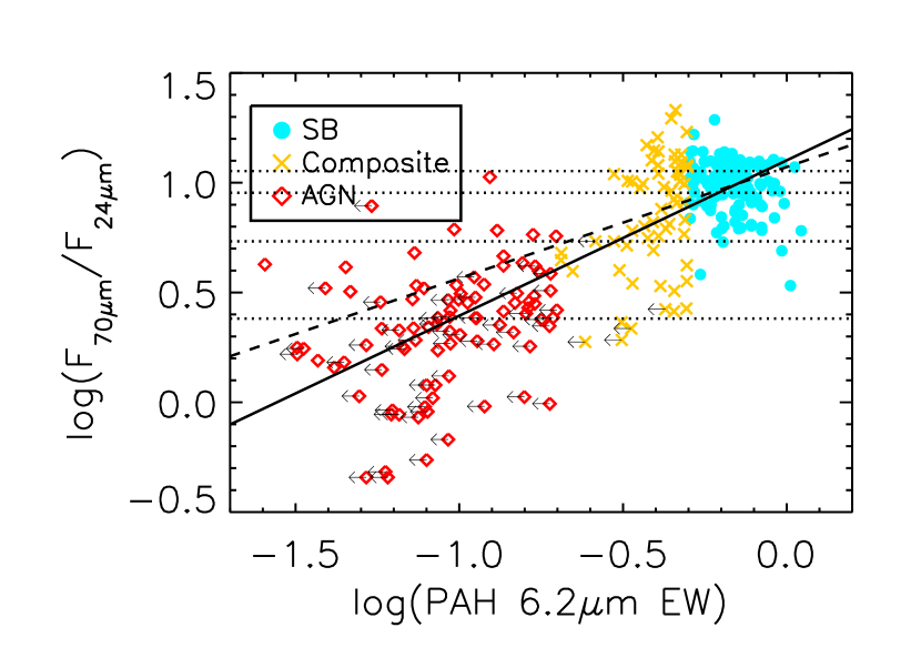
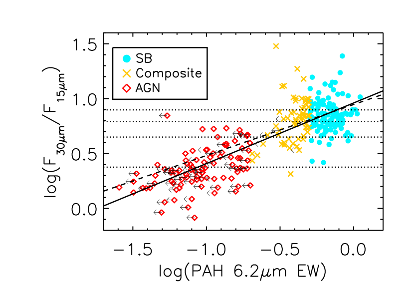
Figure 9: a) Left panel: The continuum flux ratio of f_70μm/f_24μm versus the 6.2 $\mu$m PAH EW. b) Right panel: The continuum flux ratio of f_30μm/f_15μm versus the 6.2 $\mu$m PAH EWs. The solid line is a fit to all the data points while the dashed line is a fit excluding sources with 6.2 $\mu$m PAH EW upper limits. We bin the objects according to their continuum slopes and have equal numbers of objects in each bin. The dotted lines indicate the boundaries of those bins.

In Figure 9 a and b, we plot the 6.2 $\mu$m PAH EW against $f_{\rm 30}/f_{\rm 15}$ and f₇₀/f₂₄. The 5MUSES populations separate into two groups, one with steep spectra and high aromatic content, and the other with slow rising spectra and low aromatic content. The gap between SB and AGN dominated sources is likely due to the selection effect of this sample. We should note that within each group, there is little if any correlation between the slope and the PAH EW, but it is the contrast between the two groups that gives the overall impression of a correlation. This is consistent with the studies of Veilleux et al. (2009), who have showed the power of using the 7.7 $\mu$m PAH EWs and $f_{\rm 30}/f_{\rm 15}$ ratios as indicators of AGN activity, despite the large scatter associated with each parameter. To understand the variation in the PAH EWs and continuum slopes, we further divide our sample into smaller bins and estimate the average values in each bin. The sources are divided according to their f₇₀/f₂₄ ratios or f₃₀/f₁₅ ratios and we assign an equal number of objects to each bin. We find that sources in the first three bins with log(f₃₀/f₁₅)$>$0.65 or log(f₇₀/f₂₄)$>$ 0.73 all have median 6.2 $\mu$m PAH EWs of $\sim$0.60 $\mu$m and dispersion of $\sim$0.2 dex, which again confirms our observation that within the group of starburst galaxies, there is little correlation between the slope and aromatic content. Sources with log(f₃₀/f₁₅)$<$0.38 or log(f₇₀/f₂₄)$<$0.38 are clearly AGN-dominated with very low PAH EW. The median values and the associated uncertainties of the 6.2 $\mu$m PAH EWs and continuum ratios are summarized in Table 4.

We also investigate the variation in the ratio of L_PAH/L_IR when the galaxy color indicated by the continuum slope changes. We use the sum of the PAH luminosity from the 6.2 $\mu$m, 7.7 $\mu$m complex and 11.3 $\mu$m complex to represent L_PAH, measured from the composite spectra derived for each bin. It is clear that the PAH fraction stays nearly constant for starburst dominated systems, while its contribution drops significantly when AGN becomes more dominant (see Table 4). It has been shown that the PAH luminosity can contribute $\sim$10% in star-forming galaxies (Smith et al., 2007). For our sample, we find that L_PAH contributes $\sim$5% to L_IR. This ratio is lower than the SINGS results. We have only taken the 6.2, 7.7 and 11.3 $\mu$m bands into account, while the SINGS studies include all the PAH emitting bands in the mid-IR. Since the 6.2, 7.7 and 11.3 $\mu$m bands accounts for $\sim$68% of the power in PAH emission (Smith et al., 2007), our L_PAH/L_IR ratio can be converted to $\sim$7.5% for the total PAH contribution to L_IR. This is still slightly lower than the SINGS results, but consistent within uncertainties.

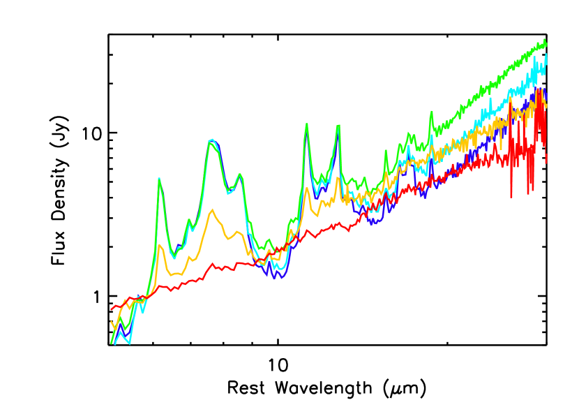
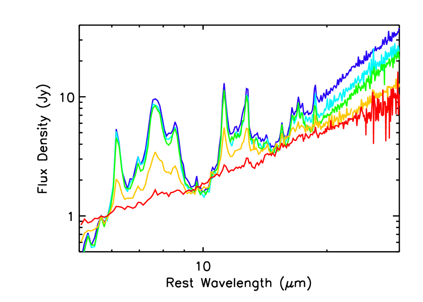
Figure 10: a) Left panel: The typical mid-IR SEDs in each bin of different f_70μm/f_24μm ratios. b) Right panel: The typical SEDs in each bin of different f_30μm/f_15μm ratios. All the SEDs have been normalized at 5.8 $\mu$m. The colors represent the average spectra derived in each f_70μm/f_24μm (or f_30μm/f_15μm) color bins listed in Table 4.

Finally, for each group of continuum slope sorted spectra, we derive typical 5-30 $\mu$m SEDs by taking the median flux densities in every wavelength bin after normalizing at rest-frame 5.8 $\mu$m. This will be useful for SED studies when only galaxy colors estimated from broad band photometry are available. These composite SEDs are shown in Figure 10. Then we explore whether the derivation of total IR luminosity from broadband photometry varies with galaxy color. We assume L_IR is correlated with L_24μm and L_70μm in the following manner and derive the a and b coefficients in each f₇₀/f₂₄ continuum slope bin (all in rest-frame):

$${\mathrm{log}}L_{\mathrm{IR}}=a~{}{\mathrm{log}}L_{\mathrm{24\mu m}}+b~{}{\mathrm{log}}L_{\mathrm{70\mu m}}$$ (1)

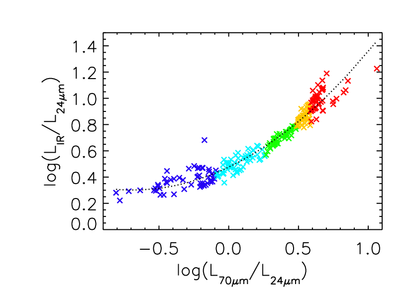
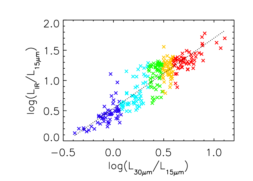
Figure 11: a) Left panel: The ratios of L_IR/L_24μm versus L_70μm/L_24μm. The sources are colored according to their f₇₀/f₂₄ ratios. The dotted line is a 2nd-order polynomial fit to the data. b) Right panel: The ratios of L_IR/L_15μm versus L_30μm/L_15μm. The sources are colored according to their f₃₀/f₁₅ ratios. The dotted line is a linear fit to the data.

The values of a and b coefficients are summarized in Table 4. To illustrate the variations in each slope bin, we plot the ratio of L_IR/L_24μm versus L_70μm/L_24μm in Figure 11 a. The sources are colored according to their f₇₀/f₂₄ ratios. We clearly observe that when normalized by the monochromatic 24 $\mu$m luminosity, L_IR is strongly correlated with L_70μm and the slopes in each continuum ratio bin become steeper when L_70μm/L_24μm increase, except in the last slope bin (see also the b coefficients). We fit a 2nd-order polynomial to the data and find the correlation to be:

$${\mathrm{log}}\frac{L_{\mathrm{IR}}}{L_{\mathrm{24\mu m}}}=(0.476\pm 0.005)+(0.509\pm 0.010)~{}{\mathrm{log}}\frac{L_{\mathrm{70\mu m}}}{L_{\mathrm{24\mu m}}}+(0.370\pm 0.022)~{}({\mathrm{log}}\frac{L_{\mathrm{70\mu m}}}{L_{\mathrm{24\mu m}}})^{2}$$ (2)

The above equation is derived based on the 5MUSES data. The majority (90%) of the 24 $\mu$m luminosities of these 280 galaxies are between 10^9.0L_⊙ and 10^12.0L_⊙. The ratio of f_70μm/f_24μm ranges from 0.45 to 34. Our result is consistent with a similar correlation derived by Papovich & Bell (2002), while it diverges for sources with low f_70μm/f_24μm ratios, since their modelling work has focused on star-forming galaxies only.

We repeat the same exercise for our sample binned with the f₃₀/f₁₅ ratios. In Figure 11 b, we find that L_IR is correlated with L_30μm when both quantities are normalized by L_15μm, although with very large scatter. The dotted line is a linear fit to the data. For a given L_30μm/L_15μm ratio, L_IR/L_15μm can span as much as a factor of five. The median values in each group binned by the f₃₀/f₁₅ ratios are also summarized in Table 4.

4.4 The Variation in PAH Band-to-Band Strength Ratios

The luminosity ratio of different PAH bands is thought to be a function of the grain size and ionization state (Tielens, 2008). luminosity ratios of L_PAH7.7μm/L_PAH11.3μm with the 6.2 $\mu$m PAH EWs for the 5MUSES sample. Only sources with S/N$>$3 from PAHFIT measurements for the 7.7 and 11.3 $\mu$m bands are included in this plot. We find that the AGN-dominated sources on average have lower L_PAH7.7μm/L_PAH11.3μm ratios than the composite or SB-dominated sources. The mean log(L_PAH7.7μm/L_PAH11.3μm) ratios for AGN, composite and SB galaxies in 5MUSES are 0.32$\pm$0.18, 0.53$\pm$0.15 and 0.53$\pm$0.08, respectively. This is consistent with the studies on the nuclear spectra of low luminosity star-forming galaxies from SINGS (Smith et al., 2007), which also show decreased L_PAH7.7μm/L_PAH11.3μm ratios in spectra with AGN signals. Smith et al. (2007) suggest that this change in the ratio of L_PAH7.7μm/L_PAH11.3μm is likely due to the destruction of the smallest PAHs by hard photons from the AGN. On the other hand, AGN are less extinguished than SB or composite sources, thus if PAHFIT underestimates the extinction correction, it will preferentially underestimate the 11.3 $\mu$m fluxes more than the 7.7 $\mu$m feature in SB/Composite sources, thus resulting in the elevated ratios of L_PAH7.7μm/L_PAH11.3μm in SB/composite systems.

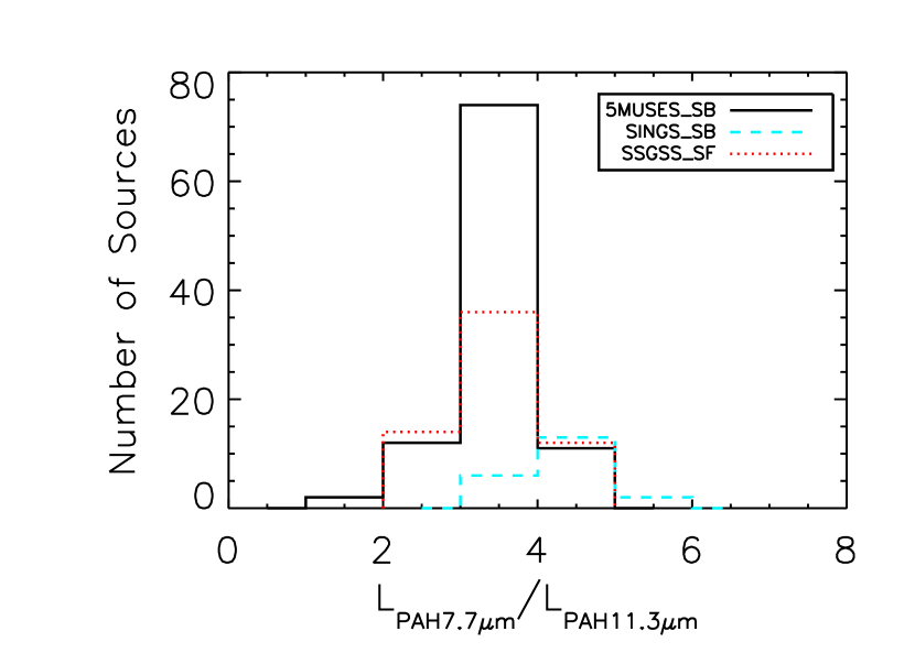
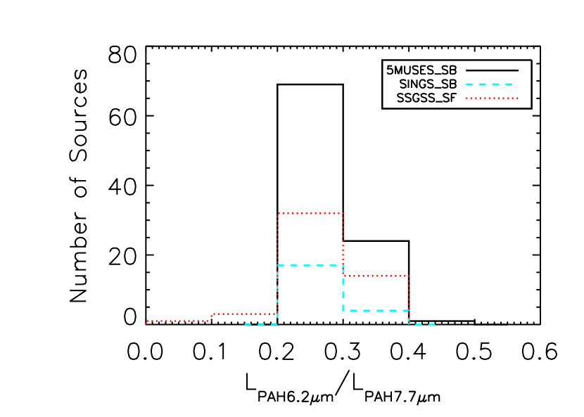
Figure 13: a) Top panel: A comparison of the distribution of PAH luminosity ratio of L_PAH7.7μm/L_PAH11.3μm for the IR classified SB-dominated sources from 5MUSES, SINGS and the optically classified SF-dominated sources in SSGSS. b) Bottom panel: Same as a), but for the PAH luminosity ratio of L_PAH6.2μm/L_PAH7.7μm. The SB and SF galaxies in 5MUSES and SSGSS appear to have a similar distribution for both the L_PAH7.7μm/L_PAH11.3μm and L_PAH6.2μm/L_PAH7.7μm ratios, while the SINGS nuclear spectra appear to show higher L_PAH7.7μm/L_PAH11.3μm ratios for the SB-dominated galaxies.

In Figure 13 a, we show the histogram of the L_PAH7.7μm/L_PAH11.3μm ratios for the SB-dominated sources in 5MUSES. We have overplotted the values from the SINGS sample. To make a fair comparison, we remeasure the PAH luminosity and EWs for the SINGS nuclear spectra using the same method as 5MUSES and classify the sources with 6.2 $\mu$m PAH EWs larger than 0.5 $\mu$m as SB-dominated. We have also included the distribution of the L_PAH7.7μm/L_PAH11.3μm ratios from the UV/SDSS selected star-forming galaxies sample of SSGSS (O’Dowd et al., 2009). For this last sample, the star-forming galaxies are classified from optical spectroscopy using the BPT diagram method (Baldwin et al., 1981; Kewley et al., 2001). We find that the distribution for SB galaxies in 5MUSES and SSGSS is similar, while both samples appear to have lower L_PAH7.7μm/L_PAH11.3μm ratios than the nuclear spectra of SINGS SB galaxies. The mean log(L_PAH7.7μm/L_PAH11.3μm) ratio for SINGS starbursts is 0.63$\pm$0.06 while it is 0.53$\pm$0.08 for 5MUSES starbursts. This might be a resolution effect: If the physical conditions at the nuclear region of a galaxy indeed modifies the distribution of the L_PAH7.7μm/L_PAH11.3μm ratios, it might be visible only in the spectra taken through apertures with small projected sizes. The median redshift for the SB-dominated sources in the 5MUSES sample is 0.12, while the median redshift for the SSGSS sample is 0.08. At the redshift of 0.08, 1$\arcsec$ corresponds to 1.53 kpc. The IRS spectra (for SL, the slit width is$\sim$3.6$\arcsec$) of 5MUSES and SSGSS sources are integrated from the whole galaxy, thus diluting the signature of the nuclear regions. Smith et al. (2007) have shown the changes in the L_PAH7.7μm/L_PAH11.3μm ratios in spectra extracted from bigger to smaller apertures in two star-forming galaxies: The L_PAH7.7μm/L_PAH11.3μm ratios measured from star-forming galaxy spectra extracted with smaller apertures are higher than those measured from larger apertures, consistent with our results. More recently, Pereira-Santaella et al. (2010) have suggested that the 11.3 $\mu$m PAH feature is more extended than the 6.2 or 7.7 $\mu$m PAH from a spatially resolved mapping study of local luminous infrared galaxies. They have observed lower L_PAH6.2μm/L_PAH11.3μm ratios in the nucleus, consistent with our results. We also show the distribution of L_PAH6.2μm/L_PAH7.7μm ratios in Figure 13 b. No significant difference has been observed between the 5MUSES, SINGS and SSGSS samples.

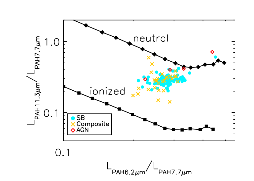
Figure 14: The PAH band-to-band ratios of L_PAH11.3μm/L_PAH7.7μm versus L_PAH6.2μm/L_PAH7.7μm. The lines represent the expected ratios for neutral (upper line) and ionized (lower line) PAHs from model predictions. Note we have fewer objects in this Figure than in Figure 12, because we require the source to have S/N$>$3 for all three PAH features (6.2, 7.7 and 11.3 $\mu$m) to be included.

Finally in Figure 14, we present the variation in PAH band-to-band ratios for the three strongest bands at 6.2, 7.7 and 11.3 $\mu$m of the 5MUSES sample. Only sources with S/N$>$3 from PAHFIT measurements for all three PAH bands are included in this figure. The two dark lines represent the traces for fully neutral or fully ionized PAH molecules with different numbers of carbon atoms predicted from modelling work (Draine & Li, 2001). The L_PAH7.7μm/L_PAH11.3μm ratios span a range of a factor of 5 while the L_PAH6.2μm/L_PAH7.7μm ratios only vary by a factor of 2. The uncertainty in the L_PAH7.7μm/L_PAH11.3μm ratios is 0.09 dex and it is 0.05 dex for the L_PAH6.2μm/L_PAH7.7μm ratios. This narrow range of L_PAH6.2μm/L_PAH7.7μm ratios is consistent with the values for the SINGS nuclear sample (Smith et al., 2007), while we have not observed any sources with extremely low L_PAH6.2μm/L_PAH7.7μm ratios ($<$0.2) as has been found in the SSGSS sample (O’Dowd et al., 2009).

4.5 PAH band ratio versus [NeIII]/[NeII]

Because of the large difference in ionization potentials of the Ne⁺⁺ (41eV) and Ne⁺ (21.6eV) ions, the ratio of [NeIII]/[NeII] is often used as a tracer of the hardness of the radiation field. The [NeIII] 15.55 $\mu$m and [NeII] 12.81 $\mu$m lines are among the strongest lines emitted in the mid-IR and because differential extinction effects between their wavelengths are small, they are particularly valuable. We use the IRS low-res spectra to identify and measure these lines. The line fluxes measured from low-resolution spectra have on average an uncertainty of $\sim$20%.

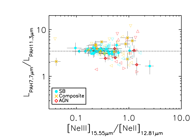
Figure 15: The flux ratios of [NeIII]/[NeII] versus the PAH luminosity ratios of L_PAH7.7μm/L_PAH11.3μm. The blue, yellow and red open triangles represent upper/lower limits for the SB, composite and AGN in 5MUSES and the directions the triangles face are consistent with the directions of the limits. The dotted line is the median L_PAH7.7μm/L_PAH11.3μm ratio for the SB-dominated sources on this plot.

In Figure 15, we show the flux ratios of L_PAH7.7μm/L_PAH11.3μm versus [NeIII]/[NeII]. The solid symbols denote detections while the open triangles represent upper/lower limits. We overplot the median L_PAH7.7μm/L_PAH11.3μm for SB-dominated sources in 5MUSES as the dotted line. We find that the SB, composite and AGN-dominated sources (including sources with upper/lower limits) are almost evenly distributed on the two sides of the dotted line. However, the AGN with solid detections on both axes do appear to have lower L_PAH7.7μm/L_PAH11.3μm ratios in general. As has been discussed in Section 4.4, this is consistent with the studies of Smith et al. (2007) using the SINGS nuclear spectra. We note that the 5MUSES sample do not have sources with extreme L_PAH7.7μm/L_PAH11.3μm ratios comparable to the lowest ones reached by SINGS. This is probably because the SINGS spectra probe smaller, more central and thus more AGN-dominated regions. It should also be noted that the AGN luminosities in 5MUSES are substantially higher than SINGS. Our results are consistent with O’Dowd et al. (2009), who have studied a UV-SDSS selected sample at z$\sim$0.1 and do not observe extreme L_PAH7.7μm/L_PAH11.3μm ratios either. We also notice that the range of [NeIII]/[NeII] ratios are similar for all three groups of objects that we have classified based on their 6.2 $\mu$m PAH EWs. This is consistent with the study of Bernard-Salas et al. (2009), who found no correlation between the PAH EWs and the [NeIII]/[NeII] ratios in a sample of starburst galaxies. However, in more extreme radiation field conditions, such as low-metallicity environment, PAH EWs have been observed to anti-correlate with the radiation field hardness indicated by [NeIII]/[NeII] ratios (Wu et al., 2006).

5 Conclusions

We have studied a flux limited (f${}_{24\mu m}>$5 mJy) representative sample of 330 galaxies surveyed with the Infrared Spectrograph on board the Spitzer Space Telescope. Secure redshifts of 280 objects have been obtained from optical or infrared spectroscopy. The redshifts of the 5MUSES sample ranges from 0.08 to 4.27, with a median value of 0.144. This places the 5MUSES sample at intermediate redshift, which bridges the gap between the nearby bright sources known from previous studies and the z$\sim$2 objects pursued in most of the IRS follow up observations of deep 24 $\mu$m surveys. The simple selection criteria ensures that our sample provides a complete census of galaxies with crucial information on understanding the galaxy evolution processes.

Using mid-IR spectroscopy and mid-to-far IR photometry, we have obtained accurate estimates on the total infrared luminosities of 5MUSES galaxies. This is achieved by minimizing the $\chi^{2}$ to find the best fit template from our newly constructed empirical SED library built upon recent Spitzer observations. The availability of longer wavelength data also greatly reduces the uncertainties in L_IR. When only one IRS spectrum is available, one can still predict the shape of the FIR SED from the mid-IR and estimate L_IR, albeit with substantially larger uncertainties (0.2 dex). The IRS-only method does not introduce a systematic bias when estimating L_IR for warm sources, but could underestimate the L_IR by $\sim$17% for cold sources, due to the lack of information sampling the peak of the SED. The fractional contribution of single band luminosity to L_IR varies depending on the dominant energy source and the average values have been calculated for the SB, composite and AGN dominated sources, as well as the whole sample.

We analyze the properties of the PAH emission in our sample using the IRS spectra. The PAH EWs show a bimodal distribution, which might be related to the selection effect of the sample. The starburst and AGN dominated sources form two clumps when comparing the continuum slopes and PAH EWs, while there is little discernible correlation within each group. Average spectra binned with the 6.2 $\mu$m PAH EWs, the continuum slopes of log(f₃₀/f₁₅) and log(f₇₀/f₂₄) have been derived to show the typical SED shapes. The variation in PAH EW and L_PAH/L_IR ratios when galaxy color changes have also been inspected. The galaxy color provides essential constraint on estimating the total infrared luminosity from broadband photometry.

We have also inspected the band-to-band PAH intensity ratios with regard to different spectral types. The L_PAH7.7μm/L_PAH11.3μm ratios in AGN dominated sources in 5MUSES are on average lower than the SB or composite sources. The SB, composite and AGN dominated sources have mean log(L_PAH7.7μm/L_PAH11.3μm) ratios of 0.53$\pm$0.08, 0.54$\pm$0.15 and 0.32$\pm$0.18, respectively. The mean log(L_PAH7.7μm/L_PAH11.3μm) ratio for the SB dominated sources in 5MUSES is lower than the mean ratio derived from the nuclear spectra of SB galaxies in SINGS (0.63$\pm$0.06), which might indicate a difference in the physical conditions near the nucleus versus over the entire galaxy. At the median redshift of our sample, the IRS SL slit width corresponds to a few kpc, thus even if the ionization state or grain size distribution is different at the nuclear level, the signal might get diluted when we study the integrated spectrum and would result in the different log(L_PAH7.7μm/L_PAH11.3μm) ratio distribution.

Finally, we provide our calibration of using PAH luminosity or mid-IR continuum luminosity to estimate L_IR in the Appendix. We have shown that single band luminosities trace the L_IR differently in SB or AGN dominated sources and we provide calibrations for each object type. This technique will be useful for luminosity estimates when no multi-wavelength data are available.

Appendix A Estimating the Total Infrared Luminosity from PAH or Monochromatic Continuum Luminosities

In Section 3, we have discussed in detail our method to estimate the total infrared luminosities for the 5MUSES sources. The empirical library of SED templates built from Spitzer observations, as well as the availability of photometric and spectroscopic data from mid-IR to FIR for 5MUSES, allow us to have precise estimates on their L_IR. We have shown in Figure 5 the importance of having FIR data in determining the total energy output in the infrared. However, for high redshift galaxies, FIR observations are not always available. Herschel Space Observatory will provide FIR measurements from 70 to 500 $\mu$m to reveal the properties of cold dust in many systems. For now, we provide our calibration of estimating L_IR from several bands in the mid-IR and discuss its applications. The following correlations are derived by performing a linear fit to the 5MUSES data with equal weight on each object because the dispersion of the data point in the x-y plane is larger than the measurement errors.

As has been shown in many studies, the infrared SED of a starburst galaxy is drastically different from that of an AGN (Brandl et al., 2006; Hao et al., 2007; Armus et al., 2007). Because of these substantial variations in the SED shapes, it is crucial to calibrate the luminosity estimates for each spectral type. Here we provide our luminosity calibrations based on the three spectral types : starburst, composite and AGN. The following PAH luminosities are derived from the PAHFIT method.

1. 6.2 $\mu$m PAH: With a wavelength cut at 28 $\mu$m for the James Webb Space Telescope (JWST), the 6.2 $\mu$m PAH feature might be the only PAH band that could be observed to quantify star formation activities in z$\sim$3 sources when JWST is launched.
For SB sources:

$${\mathrm{log}}L_{\mathrm{IR}}=(2.40\pm 0.22)+(0.96\pm 0.03){\mathrm{log}}L_{\mathrm{PAH6.2\mu m}}$$ (A1)

For composite sources:

$${\mathrm{log}}L_{\mathrm{IR}}=(1.76\pm 0.32)+(1.04\pm 0.04){\mathrm{log}}L_{\mathrm{PAH6.2\mu m}}$$ (A2)

For AGN sources:

$${\mathrm{log}}L_{\mathrm{IR}}=(-0.58\pm 0.58)+(1.30\pm 0.06){\mathrm{log}}L_{\mathrm{PAH6.2\mu m}}$$ (A3)

2. 7.7 $\mu$m PAH: The 7.7 $\mu$m PAH complex is the strongest band among the various PAH features. It is often used to estimate the total infrared luminosities for the z$\sim$1-2 sources pursued in IRS observations of 24 $\mu$m selected sources.
For SB sources:

$${\mathrm{log}}L_{\mathrm{IR}}=(2.30\pm 0.26)+(0.91\pm 0.003){\mathrm{log}}L_{\mathrm{PAH7.7\mu m}}$$ (A4)

For composite sources:

$${\mathrm{log}}L_{\mathrm{IR}}=(1.80\pm 0.44)+(0.98\pm 0.05){\mathrm{log}}L_{\mathrm{PAH7.7\mu m}}$$ (A5)

For AGN sources:

$${\mathrm{log}}L_{\mathrm{IR}}=(3.45\pm 0.90)+(0.83\pm 0.09){\mathrm{log}}L_{\mathrm{PAH7.7\mu m}}$$ (A6)

3. 11.3 $\mu$m PAH: The 11.3 $\mu$m band is another strong PAH band in the mid-IR that is relatively isolated from other PAH bands. However, the integrated fluxes from this band might be affected by the 9.7 $\mu$m silicate feature.
For SB sources:

$${\mathrm{log}}L_{\mathrm{IR}}=(2.18\pm 0.22)+(0.98\pm 0.03){\mathrm{log}}L_{\mathrm{PAH11.3\mu m}}$$ (A7)

For composite sources:

$${\mathrm{log}}L_{\mathrm{IR}}=(1.49\pm 0.43)+(1.07\pm 0.05){\mathrm{log}}L_{\mathrm{PAH11.3\mu m}}$$ (A8)

For AGN sources:

$${\mathrm{log}}L_{\mathrm{IR}}=(2.22\pm 0.36)+(1.00\pm 0.04){\mathrm{log}}L_{\mathrm{PAH11.3\mu m}}$$ (A9)

4. 6.2+7.7+11.3 $\mu$m PAH: In normal star-forming galaxies, the PAH emission accounts for $\sim$10%-15% of the total infrared luminosities (Smith et al., 2007), while this fraction is smaller for local ULIRGs (Armus et al., 2007). Here we use the sum of the three strongest PAH bands, the 6.2, 7.7 and 11.3 $\mu$m PAH luminosities to represent the total PAH luminosities. However, when using the correlation provided here, one needs to keep in mind that the properties of PAHs studied in the local universe might be different at high z, as has already been revealed in the study of several z$\sim$2 luminous infrared galaxies (Sajina et al., 2007; Pope et al., 2008). Understanding the PAH contribution in our intermediate redshift sample would also be instrumental for tackling the problem of whether and how PAH emission evolves with redshift in future studies.
For SB sources:

$${\mathrm{log}}L_{\mathrm{IR}}=(1.82\pm 0.25)+(0.95\pm 0.03){\mathrm{log}}L_{\mathrm{PAH6.2+7.7+11.3\mu m}}$$ (A10)

For composite sources:

$${\mathrm{log}}L_{\mathrm{IR}}=(0.73\pm 0.36)+(1.06\pm 0.04){\mathrm{log}}L_{\mathrm{PAH6.2+7.7+11.3\mu m}}$$ (A11)

For AGN sources:

$${\mathrm{log}}L_{\mathrm{IR}}=(-2.13\pm 1.01)+(1.35\pm 0.10){\mathrm{log}}L_{\mathrm{PAH6.2+7.7+11.3\mu m}}$$ (A12)

5. 5.8 $\mu$m monochromatic continuum luminosity: The 5.8 $\mu$m continuum luminosity provides a crude estimate of L_IR. In AGN dominated sources, the 5.8 $\mu$m continuum will be elevated due to the presence of very hot dust component. This is also a band that is available for most of the high redshift samples observed by Spitzer, and for JWST when it is launched.
For SB sources:

$${\mathrm{log}}L_{\mathrm{IR}}=(1.94\pm 0.25)+(0.95\pm 0.03){\mathrm{log}}L_{\mathrm{5.8\mu m}}$$ (A13)

For composite sources:

$${\mathrm{log}}L_{\mathrm{IR}}=(2.68\pm 0.45)+(0.87\pm 0.05){\mathrm{log}}L_{\mathrm{5.8\mu m}}$$ (A14)

For AGN sources:

$${\mathrm{log}}L_{\mathrm{IR}}=(2.34\pm 0.29)+(0.85\pm 0.03){\mathrm{log}}L_{\mathrm{5.8\mu m}}$$ (A15)

6. IRAC 8 $\mu$m: The rest-frame IRAC 8.0 $\mu$m band has included both dust continuum emission and PAH emission from the 7.7, 8.3 and 8.6 $\mu$m PAH band (if present). It provides a useful channel for estimating L_IR from PAH features when no spectroscopy is available.
For SB sources:

$${\mathrm{log}}L_{\mathrm{IR}}=(1.60\pm 0.21)+(0.93\pm 0.02){\mathrm{log}}L_{\mathrm{IRAC8\mu m}}$$ (A16)

For composite sources:

$${\mathrm{log}}L_{\mathrm{IR}}=(1.45\pm 0.26)+(0.95\pm 0.03){\mathrm{log}}L_{\mathrm{IRAC8\mu m}}$$ (A17)

For AGN sources:

$${\mathrm{log}}L_{\mathrm{IR}}=(1.70\pm 0.26)+(0.90\pm 0.02){\mathrm{log}}L_{\mathrm{IRAC8\mu m}}$$ (A18)

7. 14 $\mu$m monochromatic continuum luminosity: The 14 $\mu$m is an important band in the mid-IR that is still sensitive to the AGN emission.

For SB sources:

$${\mathrm{log}}L_{\mathrm{IR}}=(1.44\pm 0.16)+(0.97\pm 0.02){\mathrm{log}}L_{\mathrm{14\mu m}}$$ (A19)

For composite sources:

$${\mathrm{log}}L_{\mathrm{IR}}=(1.76\pm 0.37)+(0.93\pm 0.04){\mathrm{log}}L_{\mathrm{14\mu m}}$$ (A20)

For AGN sources:

$${\mathrm{log}}L_{\mathrm{IR}}=(1.62\pm 0.29)+(0.90\pm 0.03){\mathrm{log}}L_{\mathrm{14\mu m}}$$ (A21)

8. 24 $\mu$m monochromatic continuum luminosity: Here we refer to the 24 $\mu$m continuum luminosity averaged in one micron range, instead of the rest-frame MIPS 24 $\mu$m band. This is because if we use the MIPS 24 $\mu$m band, sources at z$>\sim$0.3 will be eliminated from this study due to the limited wavelength coverage of its rest-frame mid-IR spectra. The sources we use in the calibration mostly have 10¹⁰L_⊙$<$L_IR $<$10¹²L_⊙ and no quasars have been included in this calibration because of the wavelength cut. Since our sample is selected at 24 $\mu$m, it tends to favor warmer sources, which also needs to be kept in mind when using these relations.
For SB sources:

$${\mathrm{log}}L_{\mathrm{IR}}=(1.56\pm 0.23)+(0.93\pm 0.02){\mathrm{log}}L_{\mathrm{24\mu m}}$$ (A22)

For composite sources:

$${\mathrm{log}}L_{\mathrm{IR}}=(1.64\pm 0.44)+(0.91\pm 0.04){\mathrm{log}}L_{\mathrm{24\mu m}}$$ (A23)

For AGN sources:

$${\mathrm{log}}L_{\mathrm{IR}}=(1.67\pm 0.47)+(0.89\pm 0.05){\mathrm{log}}L_{\mathrm{24\mu m}}$$ (A24)

Table 1: On-Source Integration Time of the Sample

f24μm (mJy)	SL2 (second)	SL1 (second)	LL2 (second)	LL1 (second)
5$\sim$7	480	480	480	480
7$\sim$10	480	240	240	240
10$\sim$15	480	480	180	180
15$\sim$25	240	120	120	120
$>$25	120	120	60	60

Table 2: General Properties of the Sample

ID	Name	RA (J2000)	Dec (J2000)	Redshift	f24μm (mJy)	6.2$\mu$m EW	log(LIR/L⊙)
5MUSES-002	5MUSES$\_$J021503.52-042421.6	02h15m03.5s	-04d24m21.7s	0.137(2)	5.2	0.776$\pm$0.009	10.89$\pm$0.02
5MUSES-004	5MUSES$\_$J021557.11-033729.0	02h15m57.1s	-03d37m29.1s	0.032(2)	8.8	0.504$\pm$0.048	9.80$\pm$0.03
5MUSES-005	5MUSES$\_$J021638.21-042250.8	02h16m38.2s	-04d22m50.9s	0.304(2)	14.4	$<$0.094	11.54$\pm$0.02
5MUSES-006	5MUSES$\_$J021640.72-044405.1	02h16m40.7s	-04d44m05.1s	0.870(1)	14.7	$<$0.045	12.70$\pm$0.01
5MUSES-008	5MUSES$\_$J021649.71-042554.8	02h16m49.7s	-04d25m54.8s	0.143(2)	10.1	1.107$\pm$0.057	11.01$\pm$0.07
5MUSES-009	5MUSES$\_$J021657.77-032459.7	02h16m57.8s	-03d24m59.8s	0.137(1)	23.8	$<$0.062	10.90$\pm$0.03
5MUSES-010	5MUSES$\_$J021729.06-041937.8	02h17m29.1s	-04d19m37.8s	1.146(1)	8.8	$<$0.113	12.74$\pm$0.06
5MUSES-011	5MUSES$\_$J021743.01-043625.1	02h17m43.0s	-04d36m25.2s	0.784(2)	5.5	$<$0.080	12.00$\pm$0.06
5MUSES-012	5MUSES$\_$J021743.82-051751.7	02h17m43.8s	-05d17m51.8s	0.031(1)	17.1	0.645$\pm$0.080	10.11$\pm$0.03
5MUSES-013	5MUSES$\_$J021754.88-035826.4	02h17m54.9s	-03d58m26.5s	0.226(1)	10.3	0.530$\pm$0.044	11.72$\pm$0.04
5MUSES-014	5MUSES$\_$J021808.22-045845.3	02h18m08.2s	-04d58m45.3s	0.712(1)	9.1	$<$0.049	12.02$\pm$0.07
5MUSES-016	5MUSES$\_$J021830.57-045622.9	02h18m30.6s	-04d56m23.0s	1.401(1)	8.4	$<$0.083	12.67$\pm$0.10
5MUSES-018	5MUSES$\_$J021849.76-052158.2	02h18m49.8s	-05d21m58.2s	0.292(1)	5.3	0.571$\pm$0.058	11.63$\pm$0.03
5MUSES-019	5MUSES$\_$J021859.74-040237.2	02h18m59.7s	-04d02m37.2s	0.199(2)	15.9	$<$0.160	11.23$\pm$0.06
5MUSES-020	5MUSES$\_$J021909.60-052512.9	02h19m09.6s	-05d25m12.9s	0.098(2)	25.3	$<$0.194	10.74$\pm$0.02
5MUSES-021	5MUSES$\_$J021912.71-050541.8	02h19m12.7s	-05d05m41.9s	0.194(2)	6.1	0.639$\pm$0.041	11.04$\pm$0.07
5MUSES-022	5MUSES$\_$J021916.05-055726.9	02h19m16.1s	-05d57m27.0s	0.103(2)	11.0	0.198$\pm$0.027	10.71$\pm$0.05
5MUSES-023	5MUSES$\_$J021928.33-042239.8	02h19m28.3s	-04d22m39.8s	0.042(2)	17.3	0.611$\pm$0.053	10.04$\pm$0.04
5MUSES-025	5MUSES$\_$J021938.70-032508.2	02h19m38.7s	-03d25m08.3s	0.435(2)	6.8	$<$0.094	11.66$\pm$0.02
5MUSES-026	5MUSES$\_$J021939.08-051133.8	02h19m39.1s	-05d11m33.9s	0.151(2)	32.5	0.101$\pm$0.010	11.38$\pm$0.06
5MUSES-028	5MUSES$\_$J021953.04-051824.1	02h19m53.0s	-05d18m24.2s	0.072(2)	30.3	0.781$\pm$0.019	10.93$\pm$0.03
5MUSES-029	5MUSES$\_$J021956.96-052440.4	02h19m57.0s	-05d24m40.5s	0.081(2)	5.6	0.699$\pm$0.079	10.44$\pm$0.04
5MUSES-030	5MUSES$\_$J022000.22-043947.6	02h20m00.2s	-04d39m47.7s	0.350(1)	5.8	0.137$\pm$0.007	11.48$\pm$0.06
5MUSES-031	5MUSES$\_$J022005.93-031545.7	02h20m05.9s	-03d15m45.8s	1.560(2)	6.9	$<$0.178	13.17$\pm$0.05
5MUSES-032	5MUSES$\_$J022012.21-034111.8	02h20m12.2s	-03d41m11.8s	0.166(2)	6.7	$<$0.079	10.40$\pm$0.08
5MUSES-034	5MUSES$\_$J022145.09-053207.4	02h21m45.1s	-05d32m07.4s	0.008(2)	6.2	0.391$\pm$0.049	8.16$\pm$0.05
5MUSES-035	5MUSES$\_$J022147.82-025730.7	02h21m47.8s	-02d57m30.7s	0.068(2)	21.0	0.714$\pm$0.037	10.88$\pm$0.04
5MUSES-036	5MUSES$\_$J022147.87-044613.5	02h21m47.9s	-04d46m13.5s	0.025(2)	5.1	0.809$\pm$0.035	9.15$\pm$0.02
5MUSES-037	5MUSES$\_$J022151.54-032911.8	02h21m51.5s	-03d29m11.8s	0.164(1)	6.9	0.748$\pm$0.104	11.14$\pm$0.03
5MUSES-038	5MUSES$\_$J022205.03-050537.0	02h22m05.0s	-05d05m37.0s	0.258(2)	6.3	0.696$\pm$0.035	11.68$\pm$0.04
5MUSES-039	5MUSES$\_$J022223.26-044319.8	02h22m23.3s	-04d43m19.9s	0.073(2)	5.1	0.356$\pm$0.023	10.28$\pm$0.03
5MUSES-040	5MUSES$\_$J022224.06-050550.3	02h22m24.1s	-05d05m50.4s	0.149(2)	5.7	0.602$\pm$0.022	10.95$\pm$0.02
5MUSES-041	5MUSES$\_$J022241.34-045652.0	02h22m41.3s	-04d56m52.1s	0.139(2)	5.1	0.308$\pm$0.008	10.57$\pm$0.08
5MUSES-043	5MUSES$\_$J022257.96-041840.8	02h22m58.0s	-04d18m40.8s	0.239(2)	5.3	0.205$\pm$0.013	11.18$\pm$0.05
5MUSES-044	5MUSES$\_$J022301.97-052335.8	02h23m02.0s	-05d23m35.9s	0.708(2)	6.8	$<$0.054	12.77$\pm$0.04
5MUSES-045	5MUSES$\_$J022309.31-052316.1	02h23m09.3s	-05d23m16.2s	0.084(2)	5.3	$<$0.426	9.93$\pm$0.06
5MUSES-047	5MUSES$\_$J022315.58-040606.0	02h23m15.6s	-04d06m06.0s	0.199(2)	9.4	0.486$\pm$0.067	11.31$\pm$0.04
5MUSES-048	5MUSES$\_$J022329.13-043209.5	02h23m29.1s	-04d32m09.6s	0.144(2)	7.6	0.585$\pm$0.075	10.95$\pm$0.05
5MUSES-049	5MUSES$\_$J022334.65-035229.4	02h23m34.7s	-03d52m29.4s	0.176(2)	7.6	0.966$\pm$0.129	11.03$\pm$0.10
5MUSES-050	5MUSES$\_$J022345.04-054234.4	02h23m45.0s	-05d42m34.5s	0.143(2)	9.1	0.689$\pm$0.003	11.17$\pm$0.02
5MUSES-051	5MUSES$\_$J022356.49-025431.1	02h23m56.5s	-02d54m31.1s	0.451(2)	10.4	0.058$\pm$0.004	11.79$\pm$0.07
5MUSES-052	5MUSES$\_$J022413.64-042227.8	02h24m13.6s	-04d22m27.8s	0.116(2)	9.2	0.626$\pm$0.062	10.96$\pm$0.04
5MUSES-053	5MUSES$\_$J022422.48-040230.5	02h24m22.5s	-04d02m30.6s	0.171(2)	7.5	0.414$\pm$0.007	11.16$\pm$0.04
5MUSES-054	5MUSES$\_$J022431.58-052818.8	02h24m31.6s	-05d28m18.8s	2.068(2)	9.4	$\cdots$	13.02$\pm$0.25
5MUSES-055	5MUSES$\_$J022434.28-041531.2	02h24m34.3s	-04d15m31.2s	0.259(2)	6.3	0.584$\pm$0.019	11.58$\pm$0.02
5MUSES-056	5MUSES$\_$J022438.97-042706.3	02h24m39.0s	-04d27m06.4s	0.252(2)	6.6	0.156$\pm$0.034	11.30$\pm$0.06
5MUSES-057	5MUSES$\_$J022446.99-040851.3	02h24m47.0s	-04d08m51.4s	0.096(2)	5.3	0.456$\pm$0.012	10.81$\pm$0.01
5MUSES-058	5MUSES$\_$J022457.64-041417.9	02h24m57.6s	-04d14m18.0s	0.063(2)	11.9	0.476$\pm$0.035	10.59$\pm$0.04
5MUSES-060	5MUSES$\_$J022507.43-041835.7	02h25m07.4s	-04d18m35.8s	0.105(2)	6.8	0.632$\pm$0.062	10.56$\pm$0.05
5MUSES-061	5MUSES$\_$J022508.33-053917.7	02h25m08.3s	-05d39m17.7s	0.293(2)	9.6	0.025$\pm$0.002	11.55$\pm$0.05
5MUSES-062	5MUSES$\_$J022522.59-045452.2	02h25m22.6s	-04d54m52.2s	0.144(2)	10.1	0.719$\pm$0.007	11.25$\pm$0.02
5MUSES-063	5MUSES$\_$J022536.44-050011.5	02h25m36.4s	-05d00m11.6s	0.053(1)	13.7	0.709$\pm$0.051	10.77$\pm$0.11
5MUSES-064	5MUSES$\_$J022548.21-050051.5	02h25m48.2s	-05d00m51.5s	0.150(1)	8.0	0.297$\pm$0.051	11.19$\pm$0.04
5MUSES-065	5MUSES$\_$J022549.78-040024.6	02h25m49.8s	-04d00m24.7s	0.044(2)	58.5	0.438$\pm$0.009	10.64$\pm$0.03
5MUSES-066	5MUSES$\_$J022559.99-050145.3	02h26m00.0s	-05d01m45.3s	0.205(2)	5.7	0.916$\pm$0.027	11.39$\pm$0.04
5MUSES-067	5MUSES$\_$J022602.92-045306.8	02h26m02.9s	-04d53m06.8s	0.056(2)	6.4	0.669$\pm$0.028	10.13$\pm$0.03
5MUSES-068	5MUSES$\_$J022603.61-045903.8	02h26m03.6s	-04d59m03.8s	0.055(2)	31.4	0.634$\pm$0.047	10.59$\pm$0.04
5MUSES-069	5MUSES$\_$J022617.43-050443.4	02h26m17.4s	-05d04m43.5s	0.057(2)	48.7	0.168$\pm$0.005	10.77$\pm$0.04
5MUSES-070	5MUSES$\_$J022637.79-035841.6	02h26m37.8s	-03d58m41.7s	0.070(2)	13.5	0.377$\pm$0.019	10.43$\pm$0.04
5MUSES-071	5MUSES$\_$J022655.87-040302.2	02h26m55.9s	-04d03m02.5s	0.135(2)	6.9	1.026$\pm$0.179	10.59$\pm$0.05
5MUSES-073	5MUSES$\_$J022720.68-044537.1	02h27m20.7s	-04d45m37.2s	0.055(2)	73.1	0.625$\pm$0.032	11.06$\pm$0.04
5MUSES-074	5MUSES$\_$J022738.53-044702.7	02h27m38.5s	-04d47m02.8s	0.173(2)	7.1	0.918$\pm$0.032	11.13$\pm$0.03
5MUSES-075	5MUSES$\_$J022741.64-045650.5	02h27m41.6s	-04d56m50.6s	0.055(2)	11.4	0.627$\pm$0.004	10.53$\pm$0.03
5MUSES-077	5MUSES$\_$J103237.44+580845.9	10h32m37.4s	+58d08m46.0s	0.251(2)	6.1	0.394$\pm$0.060	11.74$\pm$0.04
5MUSES-079	5MUSES$\_$J103450.50+584418.2	10h34m50.5s	+58d44m18.2s	0.091(1)	20.1	0.643$\pm$0.047	10.90$\pm$0.06
5MUSES-080	5MUSES$\_$J103513.72+573444.6	10h35m13.7s	+57d34m44.6s	1.537(2)	5.5	$<$0.171	13.25$\pm$0.08
5MUSES-081	5MUSES$\_$J103527.20+583711.9	10h35m27.2s	+58d37m12.0s	0.885(2)	6.9	0.080$\pm$0.010	12.53$\pm$0.04
5MUSES-082	5MUSES$\_$J103531.46+581234.2	10h35m31.5s	+58d12m34.2s	0.176(2)	5.0	0.574$\pm$0.018	11.25$\pm$0.04
5MUSES-083	5MUSES$\_$J103542.76+583313.1	10h35m42.8s	+58d33m13.1s	0.087(2)	6.6	0.761$\pm$0.002	10.51$\pm$0.06
5MUSES-084	5MUSES$\_$J103601.81+581836.2	10h36m01.8s	+58d18m36.2s	0.100(1)	6.0	0.421$\pm$0.012	10.63$\pm$0.04
5MUSES-085	5MUSES$\_$J103606.45+581829.7	10h36m06.5s	+58d18m29.7s	0.210(1)	22.5	$<$0.068	11.41$\pm$0.02
5MUSES-086	5MUSES$\_$J103646.42+584330.6	10h36m46.4s	+58d43m30.6s	0.140(2)	6.8	0.549$\pm$0.020	10.94$\pm$0.03
5MUSES-087	5MUSES$\_$J103701.99+574414.8	10h37m02.0s	+57d44m14.8s	0.577(2)	12.8	$<$0.065	12.06$\pm$0.05
5MUSES-088	5MUSES$\_$J103724.74+580512.9	10h37m24.7s	+58d05m12.9s	1.517(1)	8.6	$<$0.158	13.02$\pm$0.06
5MUSES-089	5MUSES$\_$J103803.35+572701.5	10h38m03.4s	+57d27m01.5s	1.285(2)	15.4	$<$0.086	13.33$\pm$0.06
5MUSES-090	5MUSES$\_$J103813.90+580047.3	10h38m13.9s	+58d00m47.4s	0.205(2)	6.2	$<$0.335	10.89$\pm$0.14
5MUSES-091	5MUSES$\_$J103818.19+583556.5	10h38m18.2s	+58d35m56.5s	0.129(2)	7.8	0.312$\pm$0.018	10.50$\pm$0.03
5MUSES-093	5MUSES$\_$J103856.16+570333.9	10h38m56.2s	+57d03m33.9s	0.178(2)	5.7	0.338$\pm$0.011	10.82$\pm$0.03
5MUSES-097	5MUSES$\_$J104016.32+570846.0	10h40m16.3s	+57d08m46.1s	0.118(2)	5.2	0.661$\pm$0.003	10.87$\pm$0.02
5MUSES-098	5MUSES$\_$J104058.79+581703.3	10h40m58.8s	+58d17m03.4s	0.072(1)	10.4	$<$0.119	9.96$\pm$0.06
5MUSES-099	5MUSES$\_$J104131.79+592258.4	10h41m31.8s	+59d22m58.4s	0.925(1)	7.0	$<$0.061	12.16$\pm$0.09
5MUSES-100	5MUSES$\_$J104132.49+565953.0	10h41m32.5s	+56d59m53.0s	0.346(1)	8.3	0.454$\pm$0.044	11.74$\pm$0.04
5MUSES-101	5MUSES$\_$J104159.83+585856.4	10h41m59.8s	+58d58m56.4s	0.360(2)	21.7	$<$0.127	11.95$\pm$0.02
5MUSES-102	5MUSES$\_$J104255.66+575549.7	10h42m55.7s	+57d55m49.8s	1.468(1)	6.4	$<$0.067	13.01$\pm$0.05
5MUSES-103	5MUSES$\_$J104303.50+585718.1	10h43m03.5s	+58d57m18.1s	0.595(1)	5.4	$<$0.066	11.90$\pm$0.05
5MUSES-105	5MUSES$\_$J104432.94+564041.6	10h44m32.9s	+56d40m41.6s	0.067(1)	28.7	0.637$\pm$0.117	10.92$\pm$0.03
5MUSES-106	5MUSES$\_$J104438.21+562210.7	10h44m38.2s	+56d22m10.8s	0.025(1)	80.6	0.509$\pm$0.027	10.49$\pm$0.05
5MUSES-107	5MUSES$\_$J104454.08+574425.7	10h44m54.1s	+57d44m25.8s	0.118(1)	6.5	0.585$\pm$0.096	10.99$\pm$0.02
5MUSES-108	5MUSES$\_$J104501.73+571111.3	10h45m01.7s	+57d11m11.4s	0.390(1)	10.9	$<$0.164	11.60$\pm$0.05
5MUSES-109	5MUSES$\_$J104516.02+592304.7	10h45m16.0s	+59d23m04.7s	0.322(1)	5.1	0.094$\pm$0.005	11.39$\pm$0.07
5MUSES-110	5MUSES$\_$J104643.26+584715.1	10h46m43.3s	+58d47m15.1s	0.140(1)	5.4	0.522$\pm$0.017	10.90$\pm$0.03
5MUSES-112	5MUSES$\_$J104705.07+590728.4	10h47m05.1s	+59d07m28.5s	0.391(1)	7.0	0.032$\pm$0.003	11.39$\pm$0.10
5MUSES-114	5MUSES$\_$J104729.89+572842.9	10h47m29.9s	+57d28m42.9s	0.230(2)	6.2	0.477$\pm$0.052	11.60$\pm$0.01
5MUSES-115	5MUSES$\_$J104837.81+582642.1	10h48m37.8s	+58d26m42.2s	0.232(1)	7.6	0.729$\pm$0.022	11.68$\pm$0.02
5MUSES-116	5MUSES$\_$J104839.73+555356.4	10h48m39.7s	+55d53m56.5s	2.043(1)	9.8	$\cdots$	13.46$\pm$0.25
5MUSES-117	5MUSES$\_$J104843.90+580341.2	10h48m43.9s	+58d03m41.3s	0.162(2)	7.1	0.838$\pm$0.029	11.04$\pm$0.05
5MUSES-118	5MUSES$\_$J104907.15+565715.3	10h49m07.2s	+56d57m15.4s	0.072(1)	9.7	0.805$\pm$0.014	10.65$\pm$0.03
5MUSES-119	5MUSES$\_$J104918.33+562512.9	10h49m18.3s	+56d25m13.0s	0.330(1)	7.1	0.037$\pm$0.001	11.20$\pm$0.08
5MUSES-123	5MUSES$\_$J105005.97+561500.0	10h50m06.0s	+56d15m00.0s	0.119(2)	14.8	0.714$\pm$0.097	11.14$\pm$0.04
5MUSES-124	5MUSES$\_$J105047.83+590348.3	10h50m47.8s	+59d03m48.4s	0.131(2)	5.2	0.623$\pm$0.015	10.90$\pm$0.04
5MUSES-126	5MUSES$\_$J105058.76+560550.0	10h50m58.8s	+56d05m50.0s	0.125(2)	5.5	0.496$\pm$0.054	10.41$\pm$0.05
5MUSES-127	5MUSES$\_$J105106.12+591625.3	10h51m06.1s	+59d16m25.3s	0.768(1)	5.4	0.078$\pm$0.003	12.32$\pm$0.06
5MUSES-128	5MUSES$\_$J105128.05+573502.4	10h51m28.1s	+57d35m02.4s	0.073(1)	10.0	0.695$\pm$0.081	10.42$\pm$0.03
5MUSES-130	5MUSES$\_$J105158.53+590652.0	10h51m58.5s	+59d06m52.1s	1.814(2)	5.4	$<$0.093	13.26$\pm$0.05
5MUSES-131	5MUSES$\_$J105200.29+591933.7	10h52m00.3s	+59d19m33.8s	0.115(1)	11.4	0.297$\pm$0.036	10.76$\pm$0.03
5MUSES-132	5MUSES$\_$J105206.56+580947.1	10h52m06.6s	+58d09m47.1s	0.117(2)	16.7	0.661$\pm$0.009	11.34$\pm$0.03
5MUSES-133	5MUSES$\_$J105336.87+580350.7	10h53m36.9s	+58d03m50.7s	0.460(1)	5.9	0.368$\pm$0.001	12.02$\pm$0.04
5MUSES-135	5MUSES$\_$J105404.11+574019.7	10h54m04.1s	+57d40m19.7s	1.101(1)	8.5	$<$0.084	12.70$\pm$0.03
5MUSES-136	5MUSES$\_$J105421.65+582344.6	10h54m21.7s	+58d23m44.7s	0.205(2)	16.8	0.074$\pm$0.001	11.43$\pm$0.03
5MUSES-138	5MUSES$\_$J105604.84+574229.9	10h56m04.8s	+57d42m30.0s	1.211(1)	11.2	$<$0.146	13.16$\pm$0.11
5MUSES-139	5MUSES$\_$J105636.95+573449.3	10h56m37.0s	+57d34m49.4s	0.047(1)	6.4	0.444$\pm$0.060	10.16$\pm$0.04
5MUSES-140	5MUSES$\_$J105641.81+580046.0	10h56m41.8s	+58d00m46.0s	0.130(1)	7.5	0.686$\pm$0.014	11.03$\pm$0.03
5MUSES-141	5MUSES$\_$J105705.43+580437.4	10h57m05.4s	+58d04m37.4s	0.140(2)	16.5	0.097$\pm$0.001	11.18$\pm$0.03
5MUSES-142	5MUSES$\_$J105733.53+565737.4	10h57m33.5s	+56d57m37.5s	0.086(1)	5.6	0.454$\pm$0.023	10.38$\pm$0.06
5MUSES-143	5MUSES$\_$J105740.55+570616.4	10h57m40.6s	+57d06m16.5s	0.073(1)	6.1	0.503$\pm$0.058	10.24$\pm$0.03
5MUSES-144	5MUSES$\_$J105829.28+580439.2	10h58m29.3s	+58d04m39.3s	0.136(1)	7.1	0.452$\pm$0.075	10.56$\pm$0.03
5MUSES-145	5MUSES$\_$J105854.08+574130.0	10h58m54.1s	+57d41m30.0s	0.232(1)	6.1	0.222$\pm$0.031	11.10$\pm$0.07
5MUSES-146	5MUSES$\_$J105903.47+572155.1	10h59m03.5s	+57d21m55.1s	0.119(2)	13.8	$<$0.261	10.87$\pm$0.05
5MUSES-147	5MUSES$\_$J105951.71+581802.9	10h59m51.7s	+58d18m02.9s	2.335(1)	5.3	$\cdots$	13.08$\pm$0.17
5MUSES-148	5MUSES$\_$J105959.95+574848.1	11h00m00.0s	+57d48m48.2s	0.453(1)	9.1	$<$0.052	11.83$\pm$0.02
5MUSES-149	5MUSES$\_$J110002.06+573142.1	11h00m02.1s	+57d31m42.2s	0.387(2)	8.3	0.496$\pm$0.027	12.02$\pm$0.05
5MUSES-151	5MUSES$\_$J110124.97+574315.8	11h01m25.0s	+57d43m15.9s	0.243(1)	6.1	0.545$\pm$0.058	11.17$\pm$0.06
5MUSES-152	5MUSES$\_$J110133.80+575206.6	11h01m33.8s	+57d52m06.6s	0.277(2)	6.4	0.509$\pm$0.057	11.84$\pm$0.04
5MUSES-153	5MUSES$\_$J110223.58+574436.2	11h02m23.6s	+57d44m36.2s	0.226(1)	10.2	$<$0.093	11.12$\pm$0.02
5MUSES-154	5MUSES$\_$J110235.02+574655.7	11h02m35.0s	+57d46m55.7s	0.226(2)	6.2	0.523$\pm$0.066	11.48$\pm$0.04
5MUSES-155	5MUSES$\_$J155833.00+544426.9	15h58m32.9s	+54d44m27.2s	0.350(1)	9.1	0.086$\pm$0.001	11.52$\pm$0.03
5MUSES-156	5MUSES$\_$J155833.28+545937.1	15h58m33.3s	+54d59m37.2s	0.340(2)	6.3	0.327$\pm$0.012	12.10$\pm$0.03
5MUSES-157	5MUSES$\_$J155936.12+544203.7	15h59m36.1s	+54d42m03.8s	0.308(2)	14.5	$<$0.060	11.32$\pm$0.06
5MUSES-158	5MUSES$\_$J160038.82+551018.6	16h00m38.8s	+55d10m18.7s	0.144(2)	20.1	0.637$\pm$0.020	11.45$\pm$0.04
5MUSES-160	5MUSES$\_$J160114.49+551304.1	16h01m14.5s	+55d13m04.1s	0.220(2)	7.9	$<$0.079	10.82$\pm$0.06
5MUSES-162	5MUSES$\_$J160128.52+544521.3	16h01m28.5s	+54d45m21.4s	0.728(1)	12.8	$<$0.034	12.47$\pm$0.01
5MUSES-163	5MUSES$\_$J160322.77+544237.3	16h03m22.8s	+54d42m37.3s	0.215(1)	5.7	0.687$\pm$0.070	11.35$\pm$0.03
5MUSES-165	5MUSES$\_$J160341.30+552612.7	16h03m41.3s	+55d26m12.7s	0.146(1)	5.3	0.610$\pm$0.012	11.11$\pm$0.03
5MUSES-166	5MUSES$\_$J160358.18+555504.4	16h03m58.2s	+55d55m04.4s	0.322(2)	5.0	0.406$\pm$0.030	11.56$\pm$0.06
5MUSES-167	5MUSES$\_$J160401.21+551502.7	16h04m01.2s	+55d15m02.7s	0.182(1)	11.4	$<$0.112	11.11$\pm$0.05
5MUSES-168	5MUSES$\_$J160408.18+542531.2	16h04m08.2s	+54d25m31.2s	0.260(1)	5.0	0.604$\pm$0.054	11.54$\pm$0.02
5MUSES-169	5MUSES$\_$J160408.30+545813.0	16h04m08.3s	+54d58m13.1s	0.064(1)	26.2	0.602$\pm$0.009	10.83$\pm$0.03
5MUSES-171	5MUSES$\_$J160440.64+553409.2	16h04m40.6s	+55d34m09.3s	0.078(1)	22.9	0.521$\pm$0.035	11.10$\pm$0.04
5MUSES-173	5MUSES$\_$J160630.59+542007.4	16h06m30.6s	+54d20m07.4s	0.820(1)	5.5	$<$0.052	11.91$\pm$0.10
5MUSES-174	5MUSES$\_$J160655.35+534016.9	16h06m55.4s	+53d40m16.9s	0.214(1)	14.6	$<$0.086	11.26$\pm$0.01
5MUSES-176	5MUSES$\_$J160730.41+554905.5	16h07m30.4s	+55d49m05.6s	0.118(1)	6.2	0.835$\pm$0.100	10.81$\pm$0.03
5MUSES-177	5MUSES$\_$J160743.09+554416.5	16h07m43.1s	+55d44m16.5s	0.118(1)	9.6	0.752$\pm$0.049	11.13$\pm$0.03
5MUSES-178	5MUSES$\_$J160801.79+555359.7	16h08m01.8s	+55d53m59.7s	0.062(1)	6.2	1.057$\pm$0.011	10.24$\pm$0.04
5MUSES-179	5MUSES$\_$J160803.71+545301.9	16h08m03.7s	+54d53m02.0s	0.053(1)	5.1	0.373$\pm$0.019	10.26$\pm$0.01
5MUSES-180	5MUSES$\_$J160819.57+553314.2	16h08m19.6s	+55d33m14.3s	0.115(1)	7.2	0.337$\pm$0.005	10.83$\pm$0.02
5MUSES-181	5MUSES$\_$J160832.59+552926.9	16h08m32.6s	+55d29m27.0s	0.065(1)	5.9	0.844$\pm$0.121	10.32$\pm$0.03
5MUSES-183	5MUSES$\_$J160839.73+552330.6	16h08m39.7s	+55d23m30.7s	0.064(1)	5.8	0.964$\pm$0.029	10.33$\pm$0.02
5MUSES-184	5MUSES$\_$J160847.02+563702.2	16h08m47.0s	+56d37m02.2s	0.590(1)	8.3	0.045$\pm$0.001	12.21$\pm$0.02
5MUSES-185	5MUSES$\_$J160858.38+553010.2	16h08m58.4s	+55d30m10.3s	0.066(1)	8.8	0.586$\pm$0.104	10.34$\pm$0.02
5MUSES-186	5MUSES$\_$J160858.66+563635.6	16h08m58.7s	+56d36m35.7s	0.117(1)	5.0	0.566$\pm$0.050	10.77$\pm$0.04
5MUSES-187	5MUSES$\_$J160907.56+552428.4	16h09m07.6s	+55d24m28.4s	0.065(1)	7.7	0.670$\pm$0.003	10.54$\pm$0.03
5MUSES-188	5MUSES$\_$J160908.28+552241.4	16h09m08.3s	+55d22m41.5s	0.084(1)	6.6	0.824$\pm$0.056	10.65$\pm$0.02
5MUSES-189	5MUSES$\_$J160926.69+551642.3	16h09m26.7s	+55d16m42.3s	0.068(2)	6.8	0.507$\pm$0.058	10.19$\pm$0.02
5MUSES-190	5MUSES$\_$J160930.53+563509.0	16h09m30.5s	+56d35m09.1s	0.030(1)	5.1	0.428$\pm$0.028	9.22$\pm$0.06
5MUSES-191	5MUSES$\_$J160931.55+541827.3	16h09m31.6s	+54d18m27.4s	0.082(1)	5.6	0.497$\pm$0.033	10.61$\pm$0.04
5MUSES-192	5MUSES$\_$J160937.48+541259.2	16h09m37.5s	+54d12m59.3s	0.086(1)	5.7	0.681$\pm$0.018	10.66$\pm$0.02
5MUSES-193	5MUSES$\_$J161103.73+544322.0	16h11m03.7s	+54d43m22.1s	0.063(2)	6.6	0.536$\pm$0.018	10.26$\pm$0.03
5MUSES-194	5MUSES$\_$J161119.36+553355.4	16h11m19.4s	+55d33m55.4s	0.227(1)	35.4	$<$0.100	11.76$\pm$0.03
5MUSES-195	5MUSES$\_$J161123.44+545158.2	16h11m23.4s	+54d51m58.2s	0.078(2)	5.5	0.516$\pm$0.002	10.40$\pm$0.03
5MUSES-196	5MUSES$\_$J161223.39+540339.2	16h12m23.4s	+54d03m39.2s	0.138(2)	13.0	0.839$\pm$0.136	11.07$\pm$0.03
5MUSES-197	5MUSES$\_$J161233.43+545630.4	16h12m33.4s	+54d56m30.5s	0.083(1)	8.3	0.560$\pm$0.083	10.66$\pm$0.04
5MUSES-198	5MUSES$\_$J161241.05+543956.8	16h12m41.1s	+54d39m56.8s	0.035(2)	5.7	0.841$\pm$0.078	9.51$\pm$0.03
5MUSES-199	5MUSES$\_$J161249.54+564232.7	16h12m49.5s	+56d42m32.8s	0.336(1)	8.0	0.411$\pm$0.036	11.60$\pm$0.08
5MUSES-200	5MUSES$\_$J161250.85+532304.9	16h12m50.9s	+53d23m05.0s	0.048(2)	17.9	0.405$\pm$0.074	10.40$\pm$0.05
5MUSES-202	5MUSES$\_$J161254.17+545525.4	16h12m54.2s	+54d55m25.4s	0.065(2)	8.0	0.624$\pm$0.015	10.59$\pm$0.01
5MUSES-203	5MUSES$\_$J161301.82+552123.0	16h13m01.8s	+55d21m23.1s	0.012(2)	36.3	0.563$\pm$0.044	9.47$\pm$0.05
5MUSES-204	5MUSES$\_$J161357.01+534105.3	16h13m57.0s	+53d41m05.3s	0.180(2)	6.5	0.106$\pm$0.004	10.83$\pm$0.03
5MUSES-205	5MUSES$\_$J161402.98+560756.9	16h14m03.0s	+56d07m57.0s	0.063(2)	21.0	0.746$\pm$0.052	10.79$\pm$0.06
5MUSES-207	5MUSES$\_$J161406.87+551451.9	16h14m06.9s	+55d14m52.0s	0.564(2)	9.2	0.047$\pm$0.010	12.18$\pm$0.03
5MUSES-208	5MUSES$\_$J161411.52+540554.3	16h14m11.5s	+54d05m54.3s	0.305(1)	5.9	0.587$\pm$0.123	11.72$\pm$0.04
5MUSES-209	5MUSES$\_$J161449.08+554512.9	16h14m49.1s	+55d45m12.9s	0.064(1)	15.0	0.148$\pm$0.007	10.26$\pm$0.03
5MUSES-210	5MUSES$\_$J161521.78+543148.3	16h15m21.8s	+54d31m48.3s	0.474(1)	5.1	$<$0.058	11.47$\pm$0.08
5MUSES-211	5MUSES$\_$J161528.07+534402.4	16h15m28.1s	+53d44m02.5s	0.133(2)	6.0	0.476$\pm$0.071	11.01$\pm$0.03
5MUSES-212	5MUSES$\_$J161542.10+561814.7	16h15m42.1s	+56d18m14.7s	0.109(1)	13.7	$<$0.150	10.67$\pm$0.04
5MUSES-214	5MUSES$\_$J161546.51+550330.9	16h15m46.5s	+55d03m31.0s	0.087(1)	8.9	0.169$\pm$0.003	10.26$\pm$0.03
5MUSES-215	5MUSES$\_$J161548.31+534551.1	16h15m48.3s	+53d45m51.1s	0.147(1)	7.5	0.512$\pm$0.104	11.18$\pm$0.03
5MUSES-216	5MUSES$\_$J161551.45+541535.9	16h15m51.5s	+54d15m36.0s	0.215(2)	6.3	0.445$\pm$0.049	11.43$\pm$0.04
5MUSES-217	5MUSES$\_$J161644.45+533734.0	16h16m44.4s	+53d37m34.3s	0.147(1)	8.8	0.828$\pm$0.080	11.19$\pm$0.02
5MUSES-219	5MUSES$\_$J161645.92+542554.4	16h16m45.9s	+54d25m54.4s	0.223(1)	12.4	0.162$\pm$0.002	11.26$\pm$0.02
5MUSES-220	5MUSES$\_$J161655.96+545307.0	16h16m56.0s	+54d53m07.1s	0.418(1)	5.1	0.391$\pm$0.039	11.81$\pm$0.05
5MUSES-221	5MUSES$\_$J161659.95+560027.2	16h17m00.0s	+56d00m27.2s	0.063(1)	10.8	0.517$\pm$0.049	10.66$\pm$0.02
5MUSES-222	5MUSES$\_$J161712.27+551853.0	16h17m12.3s	+55d18m53.0s	0.037(1)	6.7	0.714$\pm$0.030	9.53$\pm$0.06
5MUSES-223	5MUSES$\_$J161716.57+550920.3	16h17m16.6s	+55d09m20.3s	0.092(2)	7.3	0.728$\pm$0.022	10.65$\pm$0.04
5MUSES-225	5MUSES$\_$J161748.06+551831.1	16h17m48.1s	+55d18m31.1s	0.145(1)	7.0	0.363$\pm$0.030	11.13$\pm$0.05
5MUSES-227	5MUSES$\_$J161759.22+541501.3	16h17m59.2s	+54d15m01.3s	0.135(1)	22.7	0.137$\pm$0.006	11.12$\pm$0.06
5MUSES-228	5MUSES$\_$J161809.36+551522.0	16h18m09.4s	+55d15m22.1s	0.136(1)	6.4	0.137$\pm$0.002	10.71$\pm$0.05
5MUSES-229	5MUSES$\_$J161819.31+541859.0	16h18m19.3s	+54d18m59.1s	0.083(1)	28.3	0.472$\pm$0.005	11.14$\pm$0.04
5MUSES-230	5MUSES$\_$J161823.11+552721.4	16h18m23.1s	+55d27m21.4s	0.084(1)	25.3	0.613$\pm$0.016	11.13$\pm$0.03
5MUSES-231	5MUSES$\_$J161827.72+552208.6	16h18m27.7s	+55d22m08.6s	0.083(1)	9.9	0.673$\pm$0.082	10.74$\pm$0.05
5MUSES-232	5MUSES$\_$J161843.35+554433.1	16h18m43.4s	+55d44m33.1s	0.153(1)	10.1	0.618$\pm$0.046	11.29$\pm$0.03
5MUSES-233	5MUSES$\_$J161848.03+535837.5	16h18m48.0s	+53d58m37.6s	0.079(1)	7.2	0.124$\pm$0.005	10.49$\pm$0.09
5MUSES-234	5MUSES$\_$J161929.57+541841.9	16h19m29.6s	+54d18m41.9s	0.100(1)	16.5	0.487$\pm$0.048	11.07$\pm$0.02
5MUSES-235	5MUSES$\_$J161950.52+543715.3	16h19m50.5s	+54d37m15.4s	0.146(1)	7.0	0.761$\pm$0.041	11.14$\pm$0.03
5MUSES-239	5MUSES$\_$J162033.98+542323.5	16h20m34.0s	+54d23m23.5s	0.133(1)	9.1	0.622$\pm$0.058	11.07$\pm$0.05
5MUSES-240	5MUSES$\_$J162038.10+553521.4	16h20m38.1s	+55d35m21.5s	0.191(1)	8.6	0.716$\pm$0.099	11.39$\pm$0.03
5MUSES-241	5MUSES$\_$J162058.82+542513.1	16h20m58.8s	+54d25m13.2s	0.082(1)	21.3	0.880$\pm$0.005	11.11$\pm$0.03
5MUSES-242	5MUSES$\_$J162059.02+542601.5	16h20m59.0s	+54d26m01.5s	0.046(1)	17.2	0.732$\pm$0.068	10.20$\pm$0.07
5MUSES-243	5MUSES$\_$J162110.51+544116.8	16h21m10.5s	+54d41m16.8s	0.155(1)	9.0	0.175$\pm$0.008	10.92$\pm$0.06
5MUSES-244	5MUSES$\_$J162127.98+551452.9	16h21m28.0s	+55d14m52.9s	0.100(1)	5.6	0.707$\pm$0.091	10.74$\pm$0.02
5MUSES-245	5MUSES$\_$J162133.00+551829.9	16h21m33.0s	+55d18m29.9s	0.238(1)	7.7	0.494$\pm$0.081	11.27$\pm$0.13
5MUSES-247	5MUSES$\_$J162150.85+553008.8	16h21m50.9s	+55d30m08.9s	0.099(1)	6.6	0.911$\pm$0.009	10.82$\pm$0.02
5MUSES-248	5MUSES$\_$J162210.87+550253.7	16h22m10.9s	+55d02m53.8s	0.034(1)	47.7	0.527$\pm$0.062	10.58$\pm$0.04
5MUSES-249	5MUSES$\_$J162214.77+550614.1	16h22m14.8s	+55d06m14.2s	0.237(1)	7.4	0.470$\pm$0.021	11.67$\pm$0.02
5MUSES-250	5MUSES$\_$J162313.11+551111.5	16h23m13.1s	+55d11m11.6s	0.236(1)	6.6	0.405$\pm$0.001	11.67$\pm$0.02
5MUSES-251	5MUSES$\_$J163001.46+410952.9	16h30m01.5s	+41d09m52.9s	0.121(1)	7.3	0.697$\pm$0.127	10.84$\pm$0.01
5MUSES-252	5MUSES$\_$J163111.27+404805.2	16h31m11.3s	+40d48m05.2s	0.258(1)	16.7	0.042$\pm$0.002	11.30$\pm$0.24
5MUSES-253	5MUSES$\_$J163128.57+404536.0	16h31m28.6s	+40d45m36.0s	0.181(1)	14.8	0.170$\pm$0.009	11.13$\pm$0.04
5MUSES-254	5MUSES$\_$J163220.40+402334.4	16h32m20.4s	+40d23m34.4s	0.079(1)	8.3	0.602$\pm$0.002	10.79$\pm$0.05
5MUSES-255	5MUSES$\_$J163308.28+403321.5	16h33m08.3s	+40d33m21.6s	0.404(1)	8.3	0.164$\pm$0.013	11.82$\pm$0.05
5MUSES-256	5MUSES$\_$J163310.92+405641.3	16h33m10.9s	+40d56m41.4s	0.136(1)	8.0	0.725$\pm$0.022	10.86$\pm$0.03
5MUSES-258	5MUSES$\_$J163317.57+403443.6	16h33m17.6s	+40d34m43.6s	0.378(1)	7.2	$<$0.073	11.46$\pm$0.03
5MUSES-260	5MUSES$\_$J163335.85+401529.1	16h33m35.9s	+40d15m29.1s	0.028(1)	30.3	0.954$\pm$0.037	10.07$\pm$0.04
5MUSES-261	5MUSES$\_$J163359.12+405304.7	16h33m59.1s	+40d53m04.7s	0.032(1)	11.9	0.474$\pm$0.027	9.92$\pm$0.03
5MUSES-262	5MUSES$\_$J163401.79+412052.5	16h34m01.8s	+41d20m52.6s	0.028(1)	47.0	0.739$\pm$0.030	10.32$\pm$0.04
5MUSES-263	5MUSES$\_$J163506.06+411038.4	16h35m06.1s	+41d10m38.5s	0.079(1)	13.5	0.462$\pm$0.001	10.83$\pm$0.03
5MUSES-264	5MUSES$\_$J163541.68+405900.6	16h35m41.7s	+40d59m00.7s	0.188(1)	10.4	$<$0.189	11.04$\pm$0.03
5MUSES-265	5MUSES$\_$J163546.87+403903.6	16h35m46.9s	+40d39m03.6s	0.122(1)	8.3	0.613$\pm$0.007	11.09$\pm$0.03
5MUSES-266	5MUSES$\_$J163608.13+410507.6	16h36m08.1s	+41d05m07.7s	0.170(1)	13.2	0.457$\pm$0.010	11.91$\pm$0.10
5MUSES-267	5MUSES$\_$J163645.27+415133.6	16h36m45.3s	+41d51m33.7s	0.081(1)	7.8	$<$0.190	10.24$\pm$0.06
5MUSES-268	5MUSES$\_$J163651.65+405600.1	16h36m51.7s	+40d56m00.2s	0.476(1)	9.6	$<$0.101	11.83$\pm$0.02
5MUSES-269	5MUSES$\_$J163705.29+413155.8	16h37m05.3s	+41d31m55.9s	0.122(2)	10.6	0.704$\pm$0.001	11.20$\pm$0.03
5MUSES-270	5MUSES$\_$J163709.31+414030.8	16h37m09.3s	+41d40m30.9s	0.760(1)	9.5	$<$0.032	12.41$\pm$0.05
5MUSES-271	5MUSES$\_$J163715.58+414933.7	16h37m15.6s	+41d49m33.7s	0.121(1)	8.8	0.580$\pm$0.012	10.95$\pm$0.03
5MUSES-272	5MUSES$\_$J163729.26+405248.5	16h37m29.3s	+40d52m48.5s	0.026(2)	19.1	0.406$\pm$0.020	10.10$\pm$0.04
5MUSES-273	5MUSES$\_$J163731.41+405155.5	16h37m31.4s	+40d51m55.6s	0.189(1)	7.6	0.404$\pm$0.045	11.44$\pm$0.05
5MUSES-274	5MUSES$\_$J163751.24+401439.9	16h37m51.2s	+40d14m39.9s	0.072(2)	11.8	0.880$\pm$0.043	10.63$\pm$0.03
5MUSES-275	5MUSES$\_$J163751.35+413027.3	16h37m51.4s	+41d30m27.3s	0.287(1)	25.8	0.131$\pm$0.011	12.04$\pm$0.04
5MUSES-276	5MUSES$\_$J163751.85+401503.9	16h37m51.9s	+40d15m04.0s	0.070(2)	8.6	0.771$\pm$0.021	10.61$\pm$0.03
5MUSES-277	5MUSES$\_$J163802.24+404653.4	16h38m02.2s	+40d46m53.4s	0.103(2)	9.1	0.204$\pm$0.005	10.56$\pm$0.06
5MUSES-278	5MUSES$\_$J163805.85+413508.1	16h38m05.9s	+41d35m08.2s	0.119(2)	10.6	0.573$\pm$0.134	11.02$\pm$0.03
5MUSES-279	5MUSES$\_$J163808.47+403213.7	16h38m08.5s	+40d32m13.8s	0.220(2)	11.9	0.486$\pm$0.015	11.69$\pm$0.05
5MUSES-280	5MUSES$\_$J163809.65+402844.7	16h38m09.6s	+40d28m44.8s	0.072(2)	17.3	0.696$\pm$0.067	10.55$\pm$0.04
5MUSES-281	5MUSES$\_$J163906.16+404003.2	16h39m06.2s	+40d40m03.3s	0.035(1)	6.7	0.719$\pm$0.007	9.82$\pm$0.03
5MUSES-282	5MUSES$\_$J164019.68+403744.4	16h40m19.7s	+40d37m44.4s	0.151(1)	10.5	$<$0.199	10.76$\pm$0.08
5MUSES-284	5MUSES$\_$J164043.69+413310.0	16h40m43.7s	+41d33m10.0s	0.155(2)	5.7	0.720$\pm$0.006	11.14$\pm$0.04
5MUSES-285	5MUSES$\_$J164046.60+412522.6	16h40m46.6s	+41d25m22.6s	0.096(2)	20.7	0.098$\pm$0.003	10.78$\pm$0.05
5MUSES-286	5MUSES$\_$J164101.35+411850.6	16h41m01.4s	+41d18m50.7s	0.099(2)	22.1	0.072$\pm$0.013	10.67$\pm$0.05
5MUSES-287	5MUSES$\_$J164115.38+410320.7	16h41m15.4s	+41d03m20.7s	0.138(2)	5.6	0.519$\pm$0.006	11.14$\pm$0.02
5MUSES-288	5MUSES$\_$J164135.27+413807.3	16h41m35.3s	+41d38m07.3s	0.395(2)	5.3	0.072$\pm$0.003	11.58$\pm$0.07
5MUSES-289	5MUSES$\_$J164153.76+405842.5	16h41m53.8s	+40d58m42.6s	0.327(2)	5.9	0.119$\pm$0.004	11.43$\pm$0.03
5MUSES-290	5MUSES$\_$J164211.92+410816.7	16h42m11.9s	+41d08m16.8s	0.144(2)	11.7	0.546$\pm$0.013	11.36$\pm$0.04
5MUSES-291	5MUSES$\_$J164214.47+405129.0	16h42m14.5s	+40d51m29.0s	0.104(2)	14.1	$<$0.058	10.62$\pm$0.01
5MUSES-292	5MUSES$\_$J171033.21+584456.8	17h10m33.2s	+58d44m56.7s	0.281(2)	6.1	0.325$\pm$0.001	11.39$\pm$0.07
5MUSES-293	5MUSES$\_$J171124.22+593121.4	17h11m24.2s	+59d31m21.5s	1.489(2)	5.6	$<$0.080	12.92$\pm$0.02
5MUSES-294	5MUSES$\_$J171232.34+592125.9	17h12m32.4s	+59d21m26.2s	0.210(2)	8.7	0.507$\pm$0.006	11.59$\pm$0.04
5MUSES-295	5MUSES$\_$J171233.38+583610.5	17h12m33.4s	+58d36m10.3s	1.663(1)	5.1	$<$0.113	13.18$\pm$0.04
5MUSES-296	5MUSES$\_$J171233.77+594026.4	17h12m33.7s	+59d40m26.8s	0.217(2)	5.      1	0.983$\pm$0.067	11.29$\pm$0.03
5MUSES-297	5MUSES$\_$J171316.50+583234.9	17h13m16.6s	+58d32m34.9s	0.079(2)	6.7	0.780$\pm$0.020	10.34$\pm$0.04
5MUSES-298	5MUSES$\_$J171325.18+590531.1	17h13m25.2s	+59d05m31.2s	0.126(1)	9.4	$<$0.189	10.33$\pm$0.06
5MUSES-299	5MUSES$\_$J171414.81+585221.5	17h14m14.8s	+58d52m21.6s	0.167(1)	9.0	0.780$\pm$0.006	11.19$\pm$0.03
5MUSES-300	5MUSES$\_$J171419.98+602724.6	17h14m20.0s	+60d27m24.8s	2.990(1)	5.6	$\cdots$	13.79$\pm$0.09
5MUSES-301	5MUSES$\_$J171430.76+584225.4	17h14m30.8s	+58d42m25.4s	0.562(2)	8.3	$<$0.075	11.70$\pm$0.06
5MUSES-302	5MUSES$\_$J171446.47+593400.1	17h14m46.4s	+59d33m59.8s	0.129(1)	7.5	0.637$\pm$0.002	11.11$\pm$0.02
5MUSES-303	5MUSES$\_$J171447.31+583805.9	17h14m47.3s	+58d38m05.8s	0.257(2)	5.4	0.836$\pm$0.012	11.60$\pm$0.04
5MUSES-304	5MUSES$\_$J171513.88+594638.1	17h15m13.8s	+59d46m38.3s	0.248(1)	5.1	0.338$\pm$0.091	11.21$\pm$0.04
5MUSES-305	5MUSES$\_$J171544.03+600835.3	17h15m44.0s	+60d08m35.2s	0.157(2)	6.9	$<$0.190	10.72$\pm$0.04
5MUSES-306	5MUSES$\_$J171550.50+593548.8	17h15m50.5s	+59d35m48.7s	0.066(2)	9.1	0.073$\pm$0.005	10.16$\pm$0.04
5MUSES-307	5MUSES$\_$J171614.48+595423.8	17h16m14.5s	+59d54m23.6s	0.153(2)	8.6	0.827$\pm$0.009	11.29$\pm$0.03
5MUSES-308	5MUSES$\_$J171630.23+601422.7	17h16m30.2s	+60d14m22.7s	0.107(1)	8.6	0.833$\pm$0.133	10.75$\pm$0.05
5MUSES-309	5MUSES$\_$J171650.58+595751.4	17h16m50.6s	+59d57m52.0s	0.182(1)	6.8	$<$0.313	10.74$\pm$0.10
5MUSES-310	5MUSES$\_$J171711.11+602710.0	17h17m11.1s	+60d27m10.0s	0.110(1)	9.5	0.488$\pm$0.053	10.78$\pm$0.06
5MUSES-311	5MUSES$\_$J171747.51+593258.1	17h17m47.5s	+59d32m58.1s	0.248(2)	5.3	$<$0.093	10.76$\pm$0.12
5MUSES-312	5MUSES$\_$J171754.62+600913.8	17h17m54.6s	+60d09m13.4s	4.270(1)	9.1	$\cdots$	14.59$\pm$0.13
5MUSES-313	5MUSES$\_$J171852.71+591432.0	17h18m52.7s	+59d14m32.1s	0.322(2)	14.0	0.112$\pm$0.010	11.85$\pm$0.05
5MUSES-314	5MUSES$\_$J171913.57+584509.1	17h19m13.5s	+58d45m08.9s	0.318(2)	8.8	$<$0.243	11.42$\pm$0.12
5MUSES-315	5MUSES$\_$J171933.37+592742.8	17h19m33.3s	+59d27m42.7s	0.139(2)	7.6	0.495$\pm$0.005	11.28$\pm$0.07
5MUSES-316	5MUSES$\_$J171944.91+595707.7	17h19m44.9s	+59d57m07.1s	0.069(2)	14.4	0.753$\pm$0.005	10.73$\pm$0.05
5MUSES-317	5MUSES$\_$J172043.28+584026.6	17h20m43.3s	+58d40m26.9s	0.125(2)	9.7	0.498$\pm$0.006	11.14$\pm$0.03
5MUSES-318	5MUSES$\_$J172044.86+582924.0	17h20m44.9s	+58d29m23.9s	1.697(1)	5.3	$<$0.094	13.07$\pm$0.05
5MUSES-319	5MUSES$\_$J172159.43+595034.3	17h21m59.3s	+59d50m34.2s	0.028(2)	9.7	0.387$\pm$0.031	9.78$\pm$0.03
5MUSES-320	5MUSES$\_$J172219.58+594506.9	17h22m19.6s	+59d45m07.0s	0.272(2)	7.8	$<$0.133	11.24$\pm$0.02
5MUSES-321	5MUSES$\_$J172228.04+601526.0	17h22m28.2s	+60d15m26.2s	0.742(2)	7.2	$<$0.111	12.40$\pm$0.03
5MUSES-322	5MUSES$\_$J172238.73+585107.0	17h22m38.8s	+58d51m07.0s	1.624(1)	6.7	$<$0.062	13.12$\pm$0.04
5MUSES-323	5MUSES$\_$J172313.06+590533.1	17h23m13.1s	+59d05m33.1s	0.108(2)	6.2	0.750$\pm$0.037	10.85$\pm$0.03
5MUSES-324	5MUSES$\_$J172355.58+601301.7	17h23m55.5s	+60d13m01.1s	0.175(2)	5.4	0.905$\pm$0.034	11.13$\pm$0.02
5MUSES-325	5MUSES$\_$J172355.97+594047.6	17h23m56.0s	+59d40m47.4s	0.030(2)	5.2	0.518$\pm$0.098	9.35$\pm$0.04
5MUSES-326	5MUSES$\_$J172402.11+600601.4	17h24m02.1s	+60d06m01.2s	0.156(2)	8.0	0.461$\pm$0.024	11.13$\pm$0.03
5MUSES-328	5MUSES$\_$J172546.80+593655.3	17h25m46.8s	+59d36m55.3s	0.035(2)	26.0	0.554$\pm$0.041	10.49$\pm$0.04
5MUSES-329	5MUSES$\_$J172551.35+601138.9	17h25m51.3s	+60d11m38.9s	0.029(1)	27.3	0.454$\pm$0.005	10.25$\pm$0.03
5MUSES-330	5MUSES$\_$J172619.80+601600.1	17h26m19.8s	+60d16m00.0s	0.924(1)	6.5	$<$0.039	12.35$\pm$0.08

Table 3: Median Luminosity Ratios of the Sample

	SB	composite	AGN	Whole Sample
log(LPAH6.2μm/LIR)	-2.03$\pm$0.13	-2.11$\pm$0.13	-2.22$\pm$0.14	-2.06$\pm$0.14
log(LPAH7.7μm/LIR)	-1.51$\pm$0.15	-1.54$\pm$0.18	-1.76$\pm$0.28	-1.53$\pm$0.20
log(LPAH11.3μm/LIR)	-2.04$\pm$0.13	-2.14$\pm$0.20	-2.20$\pm$0.18	-2.08$\pm$0.17
log(LPAH6.2+7.7+11.3μm/LIR)	-1.29$\pm$0.14	-1.33$\pm$0.12	-1.39$\pm$0.19	-1.31$\pm$0.14
log(L5.8μm/LIR)	-1.44$\pm$0.15	-1.36$\pm$0.29	-0.77$\pm$0.32	-1.33$\pm$0.42
log(LIRAC8μm/LIR)	-0.90$\pm$0.13	-0.96$\pm$0.15	-0.66$\pm$0.23	-0.86$\pm$0.22
log(L14μm/LIR)	-1.19$\pm$0.10	-1.11$\pm$0.21	-0.57$\pm$0.19	-1.12$\pm$0.31
log(L24μm/LIR)	-0.87$\pm$0.14	-0.82$\pm$0.23	-0.49$\pm$0.15	-0.81$\pm$0.22

Table 4: Median PAH strengths and Continuum Ratios of the Sample

log(f30/f15)	log(f70/f24)	6.2 $\mu$m PAH EW	log(LPAH/LIR)	a	b
$>$0.898	0.99${}^{+0.08}_{-0.17}$	0.57${}^{+0.18}_{-0.16}$ (56)	-1.40	0.65$\pm$0.10	0.94$\pm$0.14
0.793$-$0.898	0.97${}^{+0.11}_{-0.18}$	0.62${}^{+0.21}_{-0.13}$ (56)	-1.31	0.79$\pm$0.33	0.74$\pm$0.61
0.650$-$0.793	1.04${}^{+0.05}_{-0.35}$	0.58${}^{+0.17}_{-0.28}$ (55)	-1.29	0.70$\pm$0.28	0.94$\pm$0.65
0.376$-$0.650	0.57${}^{+0.42}_{-0.21}$	0.19${}^{+0.36}_{-0.09}$ (55)	-1.54	0.41$\pm$0.07	1.72$\pm$0.31
$<$0.376	0.25${}^{+0.21}_{-0.29}$	0.08${}^{+0.05}_{-0.04}$ (53)	-2.09	0.50$\pm$0.03	1.04$\pm$0.18
0.76${}^{+0.13}_{-0.23}$	$>$1.053	0.61${}^{+0.15}_{-0.14}$ (56)	-1.29	0.62$\pm$0.07	0.57$\pm$0.10
0.69${}^{+0.18}_{-0.35}$	0.954$-$1.053	0.61${}^{+0.15}_{-0.14}$ (56)	-1.31	0.33$\pm$0.10	0.99$\pm$0.18
0.85${}^{+0.18}_{-0.42}$	0.733$-$0.954	0.60${}^{+0.18}_{-0.21}$ (55)	-1.36	0.41$\pm$0.02	0.52$\pm$0.06
0.61${}^{+0.32}_{-0.31}$	0.381$-$0.733	0.16${}^{+0.25}_{-0.08}$ (56)	-1.60	0.47$\pm$0.01	0.52$\pm$0.06
0.57${}^{+0.31}_{-0.30}$	$<$0.381	0.08${}^{+0.08}_{-0.03}$ (52)	-2.07	0.44$\pm$0.02	0.23$\pm$0.04

Figure 2: The histogram of the flux ratios between the source and the best-fit template, for galaxies with MIPS 70 and 160 $\mu$m detections (solid line) and for galaxies only with MIPS 70 $\mu$m detections (dashed line). The dotted and dash-dotted lines indicate the medians of the flux ratios for sources with 70 and 160 $\mu$m detections and sources with only 70 $\mu$m detections. All five bands appear to peak around a log[(F(source)/F(template)] ratio of 0 with rather narrow distributions. The 1$\sigma$ deviations in F(source)/F(template) for the 5.8, 8.0, 24 and 70 160 $\mu$m bands are 0.07, 0.07, 0.03, 0.06 and 0.10 dex respectively for sources with 70 and 160 $\mu$m detections and 0.07, 0.07, 0.03 and 0.07 dex for sources with only 70 $\mu$m detections.

Figure 8: The histogram shows the distribution of the 6.2 $\mu$m PAH EW for the 280 known-z sources from the 5MUSES sample. The solid line represents sources which have detection for the 6.2 $\mu$m feature, while the dotted line includes upper limits. It is clear that both the solid line and dotted line show a dip in the PAH EW distribution at 0.2$\sim$0.3 $\mu$m. See the text for detailed discussion on the bi-modality of the distribution.

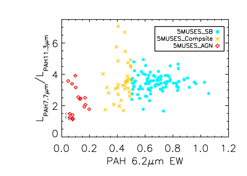
Figure 12: The PAH luminosity ratio of L_PAH7.7μm/L_PAH11.3μm versus the 6.2 $\mu$m PAH EW for 5MUSES. The AGN-dominated sources appear to have lower L_PAH7.7μm/L_PAH11.3μm ratios than the composite or SB dominated sources. The mean ratios are 3.45$\pm$0.55, 3.65$\pm$1.28 and 2.26$\pm$0.89 respectively for SB, composite and AGN.

References

- Allamandola et al. (1989) Allamandola, L. J., Tielens, A. G. G. M., & Barker, J. R. 1989, ApJS, 71, 733
- Armus et al. (2007) Armus, L., et al. 2007, ApJ, 656, 148
- Baldwin et al. (1981) Baldwin, J. A., Phillips, M. M., & Terlevich, R. 1981, PASP, 93, 5
- Bavouzet et al. (2008) Bavouzet, N., Dole, H., Le Floc’h, E., Caputi, K. I., Lagache, G., & Kochanek, C. S. 2008, A&A, 479, 83
- Bernard-Salas et al. (2009) Bernard-Salas, J., et al. 2009, ApJS, 184, 230
- Brandl et al. (2006) Brandl, B. R., et al. 2006, ApJ, 653, 1129
- Calzetti et al. (2010) Calzetti et al. 2010, ApJ, 714, 1256
- Caputi et al. (2007) Caputi, K. I., et al. 2007, ApJ, 660, 97
- Chary & Elbaz (2001) Chary, R., & Elbaz, D. 2001, ApJ, 556, 562
- Dale & Helou (2002) Dale, D. A., & Helou, G. 2002, ApJ, 576, 159
- Dale et al. (2007) Dale, D. A., et al. 2007, ApJ, 655, 863
- Dale et al. (2009) Dale, D. A., et al. 2009, ApJ, 693, 1821
- Dasyra et al. (2009) Dasyra, K. M., et al. 2009, ApJ, 701, 1123
- Desai et al. (2007) Desai, V., et al. 2007, ApJ, 669, 810
- Dey et al. (2008) Dey, A., et al. 2008, ApJ, 677, 943
- Dickinson et al. (2004) Dickinson, M., et al. 2004, ApJ, 600, L99
- Draine & Li (2007) Draine, B. T., & Li, A. 2007, ApJ, 657, 810
- Draine & Li (2001) Draine, B. T., & Li, A. 2001, ApJ, 551, 807
- Elbaz et al. (1999) Elbaz, D., et al. 1999, A&A, 351, L37
- Engelbracht et al. (2008) Engelbracht, C. W., Rieke, G. H., Gordon, K. D., Smith, J.-D. T., Werner, M. W., Moustakas, J., Willmer, C. N. A., & Vanzi, L. 2008, ApJ, 678, 804
- Fadda et al. (2006) Fadda, D., et al. 2006, AJ, 131, 2859
- Galliano et al. (2008) Galliano, F., Madden, S. C., Tielens, A. G. G. M., Peeters, E., & Jones, A. P. 2008, ApJ, 679, 310
- Genzel et al. (1998) Genzel, R., et al. 1998, ApJ, 498, 579
- Gordon et al. (2008) Gordon, K. D., Engelbracht, C. W., Rieke, G. H., Misselt, K. A., Smith, J.-D. T., & Kennicutt, R. C., Jr. 2008, ApJ, 682, 336
- Hao et al. (2007) Hao, L., Weedman, D. W., Spoon, H. W. W., Marshall, J. A., Levenson, N. A., Elitzur, M., & Houck, J. R. 2007, ApJ, 655, L77
- Higdon et al. (2004) Higdon, S. J. U., et al. 2004, PASP, 116, 975
- Hony et al. (2001) Hony, S., Van Kerckhoven, C., Peeters, E., Tielens, A. G. G. M., Hudgins, D. M., & Allamandola, L. J. 2001, A&A, 370, 1030
- Helou et al. (2001) Helou, G., Malhotra, S., Hollenbach, D. J., Dale, D. A., & Contursi, A. 2001, ApJ, 548, L73
- Houck et al. (2004) Houck, J. R., et al. 2004, ApJS, 154, 18
- Houck et al. (2005) Houck, J. R., et al. 2005, ApJ, 622, L105
- Huang et al. (2009) Huang, J.-S., et al. 2009, ApJ, 700, 183
- Kartaltepe et al. (2010) Kartaltepe, J. S., et al. 2010, ApJ, 709, 572
- Kennicutt et al. (2003) Kennicutt, R. C., Jr., et al. 2003, PASP, 115, 928
- Kewley et al. (2001) Kewley, L. J., Dopita, M. A., Sutherland, R. S., Heisler, C. A., & Trevena, J. 2001, ApJ, 556, 121
- Lacy et al. (2004) Lacy, M., et al. 2004, ApJS, 154, 166
- Laurent et al. (2000) Laurent, O., Mirabel, I. F., Charmandaris, V., Gallais, P., Madden, S. C., Sauvage, M., Vigroux, L., & Cesarsky, C. 2000, A&A, 359, 887
- Le Floc’h et al. (2005) Le Floc’h, E., et al. 2005, ApJ, 632, 169
- Lonsdale et al. (2003) Lonsdale, C. J., et al. 2003, PASP, 115, 897
- Madden et al. (2006) Madden, S. C., Galliano, F., Jones, A. P., & Sauvage, M. 2006, A&A, 446, 877
- O’Dowd et al. (2009) O’Dowd, M. J., et al. 2009, ApJ, 705, 885
- Papovich & Bell (2002) Papovich, C., & Bell, E. F. 2002, ApJ, 579, L1
- Papovich et al. (2007) Papovich, C., et al. 2007, ApJ, 668, 45
- Peeters et al. (2002) Peeters, E., Hony, S., Van Kerckhoven, C., Tielens, A. G. G. M., Allamandola, L. J., Hudgins, D. M., & Bauschlicher, C. W. 2002, A&A, 390, 1089
- Peeters et al. (2004) Peeters, E., Spoon, H. W. W., & Tielens, A. G. G. M. 2004, ApJ, 613, 986
- Pereira-Santaella et al. (2010) Pereira-Santaella et al. 2010, ApJS, 188, 447
- Pope et al. (2008) Pope, A., et al. 2008, ApJ, 675, 1171
- Puget et al. (1985) Puget, J. L., Leger, A., & Boulanger, F. 1985, A&A, 142, L19
- Rieke et al. (2004) Rieke, G. H., et al. 2004, ApJS, 154, 25
- Rieke & Low (1972) Rieke, G. H., & Low, F. J. 1972, ApJ, 176, L95
- Rieke et al. (2009) Rieke, G. H., Alonso-Herrero, A., Weiner, B. J., Pérez-González, P. G., Blaylock, M., Donley, J. L., & Marcillac, D. 2009, ApJ, 692, 556
- Roche et al. (1991) Roche, P. F., Aitken, D. K., Smith, C. H., & Ward, M. J. 1991, MNRAS, 248, 606
- Sajina et al. (2007) Sajina, A., Yan, L., Armus, L., Choi, P., Fadda, D., Helou, G., & Spoon, H. 2007, ApJ, 664, 713
- Sanders et al. (1988) Sanders, D. B., Soifer, B. T., Elias, J. H., Neugebauer, G., & Matthews, K. 1988, ApJ, 328, L35
- Sanders & Mirabel (1996) Sanders, D. B., & Mirabel, I. F. 1996, ARA&A, 34, 749
- Shi et al. (2007) Shi, Y., et al. 2007, ApJ, 669, 841
- Smith et al. (2004) Smith, J. D. T., et al. 2004, ApJS, 154, 199
- Smith et al. (2007) Smith, J. D. T., et al. 2007, ApJ, 656, 770
- Spoon et al. (2004) Spoon, H. W. W., et al. 2004, ApJS, 154, 184
- Soifer et al. (1989) Soifer, B. T., Boehmer, L., Neugebauer, G., & Sanders, D. B. 1989, AJ, 98, 766
- Spoon et al. (2007) Spoon, H. W. W., Marshall, J. A., Houck, J. R., Elitzur, M., Hao, L., Armus, L., Brandl, B. R., & Charmandaris, V. 2007, ApJ, 654, L49
- Stern et al. (2005) Stern, D., et al. 2005, ApJ, 631, 163
- Symeonidis et al. (2008) Symeonidis, M., Willner, S. P., Rigopoulou, D., Huang, J.-S., Fazio, G. G., & Jarvis, M. J. 2008, MNRAS, 385, 1015
- Tielens (2008) Tielens, A. G. G. M. 2008, ARA&A, 46, 289
- Veilleux et al. (2009) Veilleux, S., et al. 2009, ApJS, 182, 628
- Weedman et al. (2005) Weedman, D. W., et al. 2005, ApJ, 633, 706
- Weedman et al. (2006) Weedman, D. W., et al. 2006, ApJ, 651, 101
- Werner et al. (2004) Werner, M. W., et al. 2004, ApJS, 154, 1
- Wu et al. (2006) Wu, Y., Charmandaris, V., Hao, L., Brandl, B. R., Bernard-Salas, J., Spoon, H. W. W., & Houck, J. R. 2006, ApJ, 639, 157
- Wu et al. (2009) Wu, Y., Charmandaris, V., Huang, J., Spinoglio, L., & Tommasin, S. 2009, ApJ, 701, 658
- Yan et al. (2005) Yan, L., et al. 2005, ApJ, 628, 604
- Yan et al. (2007) Yan, L., et al. 2007, ApJ, 658, 778