Point mass insertion on the real line and non-exponential perturbation of the recursion coefficients

Abstract.

We present the construction of a probability measure $d\gamma$ with compact support on $\mathbb{R}$ such that adding a discrete pure point results in changes in the recursion coefficients without exponential decay.

1. Introduction

Suppose $d\mu$ is a probability measure on the unit circle $\partial\mathbb{D}$. We define an inner product and a norm on $L^{2}(\partial\mathbb{D},d\mu)$ respectively as follows:

$$\left\langle f,g\right\rangle = \displaystyle\int_{\partial\mathbb{D}}\overline{f(e^{i\theta})}g(e^{i\theta})d\mu(\theta)$$ (1.1)

$$\|f\|_{d\mu} = \left(\displaystyle\int_{\partial\mathbb{D}}|f(e^{i\theta})|^{2}d\mu(\theta)\right)^{1/2}$$ (1.2)

Using the inner product defined above, we can orthogonalize $1,z,z^{2},\dots$ to obtain the family of monic orthogonal polynomials associated with the measure $d\mu$, namely, $(\Phi_{n}(z,d\mu))_{n}$. We denote the normalized family as $(\varphi_{n}(z,d\mu))_{n}$.

Closely related to $\Phi_{n}(z)$ is the family of reversed polynomials, defined as $\Phi_{n}^{*}(z)=z^{n}\overline{\Phi_{n}(1/\overline{z})}$. They obey the well-known Szegő recursion relation

$$\Phi_{n+1}(z)=z\Phi_{n}(z)-\overline{\alpha_{n}}\Phi_{n}^{*}(z)$$ (1.3)

and $\alpha_{n}$ is known as the $n$-th Verblunsky coefficient. The Szegő recursion relations for the normalized family of orthogonal polynomials is

$$\varphi_{n+1}(z) =(1-|\alpha_{n}|^{2})^{-1/2}(z\varphi_{n}(z)-\overline{\alpha_{n}}\varphi_{n}^{*}(z))$$ (1.4)

These recursion relations will be useful later in this paper.

Now we turn to a probability measure $d\gamma$ on $\mathbb{R}$. We can define an inner product and norm on $L^{2}(\mathbb{R},d\gamma)$ as in (1.1) and (1.2), except that in this case it does not involve any conjugation. By the Gram–Schmidt process, we can orthogonalize $1,x,x^{2},\dots$ and form the family of monic orthogonal polynomials, $(P_{n}(x))_{n=0}^{\infty}$. Upon normalization, we obtain the family of orthonormal polynomials, $(p_{n}(x))_{n=0}^{\infty}$. These polynomials satisfy the following three-term recursion relation

$$xp_{n}(x)=a_{n+1}p_{n+1}(x)+b_{n+1}p_{n}(x)+a_{n}p_{n-1}(x)$$ (1.5)

where $a_{n}$ and $b_{n}$ are real numbers with $a_{n}>0$. They are called the recursion coefficients of $d\gamma$.

The main result of this paper is as follows:

Theorem 1.1.

There exists a purely absolutely continuous measure $d\gamma_{0}$ supported on $[-2,2]$ with no eigenvalues outside of $[-2,2]$, such that if we add a pure point $x_{0}\in\mathbb{R}\backslash[-2,2]$ in the following manner

$$d\tilde{\gamma}(x)=(1-\beta)d\gamma_{0}(x)+\beta\delta_{x_{0}}\quad\quad\beta>0$$ (1.6)

it will result in non-exponential perturbation of the recursion coefficients $a_{n}(d\gamma_{0})$ and $b_{n}(d\gamma_{0})$.

This example is of particular interest because of the following history: back in 1946, Borg [1] proved a well-known result concerning the Sturm–Liouville problem that in general, a single spectrum is insufficient to determine the potential. Later, Gel’fand–Levitan [8] showed that in order to recover the potential one also needs the norming constants.

Norming constants correspond to the weights of pure points and it is known that in the short range case (in orthogonal polynomials language, $a_{n}-1,b_{n}\to 0$ fast), varying the norming constants will result in exponential change in the potential.

Moreover, when considering the effect of varying the weight of discrete point masses on orthogonal polynomials (both on $\mathbb{R}$ and $\partial\mathbb{D}$), Simon proved that it will result in exponential perturbation of the recursion coefficients (see Corollary 24.4 and Corollary 24.3 of [15]).

All the results mentioned above lend to a few the intuition that if the recursion coefficients $a_{n}\to 1$ and $b_{n}\to 0$ fast, then adding a pure point will result in exponential change in the recursion coefficients. However, it turned out not to be the case!

2. Tools Involved in the Proof

2.1. The Szegő Mapping

It turns out that one can relate measures supported on $[-2,2]$ with a certain class of measures on $\partial\mathbb{D}$.

Note that the map $\theta\mapsto 2\cos\theta$ is a two-one map from $\partial\mathbb{D}$ to $[-2,2]$. Therefore, given a non-trivial probability measure $d\xi$ on $\partial\mathbb{D}$ that is invariant under $\theta\rightarrow-\theta$, we can define a measure

$$d\gamma={\rm Sz}(d\xi)$$ (2.1)

using what is known as the Szegő map, such that for $g$ measurable on $[-2,2]$,

$$\int g(2\cos\theta)d\xi(\theta)=\displaystyle\int g(x)d\gamma(x)$$ (2.2)

Conversely, if we have a probability measure $\beta$ supported on $[-2,2]$, we can obtain a probability measure

$$\nu={\rm Sz^{-1}}(d\gamma)$$ (2.3)

on $\partial\mathbb{D}$ by what is known as the Inverse Szegő Mapping, such that for $h(z)$ measurable on $\partial\mathbb{D}$,

$$\int h(\theta)d\nu(\theta)=\int h\left(\cos^{-1}\frac{x}{2}\right)d\gamma(x)$$ (2.4)

There are many interesting results about the Szegő mapping (see Chapter 13 of [14]), but the only relevant one for this paper is the following by Geronimus [9] (see also Theorem 13.1.7 of [14]):

Theorem 2.1 (Geronimus [10]).

Let $d\xi$ be a probability measure on $\partial\mathbb{D}$ which is invariant under $\theta\rightarrow-\theta$ and let $d\gamma={\rm Sz}(\xi)$. Let $\alpha_{n}\equiv\alpha_{n}(d\xi)$, $a_{n}\equiv a_{n}(d\gamma)$ and $b_{n}\equiv b_{n}(d\gamma)$. Then for $n=0,1,2,\dots$,

$$a_{n+1}^{2} = (1-\alpha_{2n-1})(1-\alpha_{2n})^{2}(1+\alpha_{2n+1})$$ (2.5)

$$b_{n+1} = (1-\alpha_{2n-1})\alpha_{2n}-(1+\alpha_{2n-1})\alpha_{2n-2}$$ (2.6)

with the convention that $\alpha_{-1}=-1$.

2.2. The Point Mass Formuula

We add a point mass $\zeta=e^{i\omega}\in\partial\mathbb{D}$ with weight $0<\beta<1$ to $d\mu$ in the following manner:

$$d\nu=(1-\beta)d\mu+\beta\delta_{\omega}$$ (2.7)

Our goal is to investigate $\alpha_{n}(d\nu)$.

Point mass perturbation has a long history (see the Introduction of [17]). One of the classic results is the following theorem:

Theorem 2.2 (Geronimus [10, 11]).

Suppose the probability measure is defined as in (2.7). Then

$$\Phi_{n}(z,d\nu)=\Phi_{n}(z)-\displaystyle\frac{\varphi_{n}(\zeta)K_{n-1}(z,\zeta)}{(1-\beta)\beta^{-1}+K_{n-1}(\zeta,\zeta)}$$ (2.8)

where

$$K_{n}(z,\zeta)=\displaystyle\sum_{j=0}^{n}\overline{\varphi_{j}(\zeta)}\varphi_{j}(z)$$ (2.9)

and all objects without the label $(d\nu)$ are associated with the measure $d\mu$.

Since $\Phi_{n}(0)=-\overline{\alpha_{n-1}}$, by putting $z=0$ into (2.8) one gets a formula relating the Verblunsky coefficients of $d\mu$ and $d\nu$. For more on the formula (2.8), the reader may refer to Nevai [13, 12], and Cachafeiro–Marcellán [3, 2, 6, 4, 5].

Using a totally different approach, Simon [14] found the following formula for OPUC:

$$\alpha_{n}(d\nu)=\alpha_{n}-q_{n}^{-1}\beta\overline{\varphi_{n+1}(\zeta)}\left(\displaystyle\sum_{j=0}^{n}\alpha_{j-1}\frac{\|\Phi_{n+1}\|}{\|\Phi_{j}\|}\varphi_{j}(\zeta)\right)$$ (2.10)

where $q_{n}=(1-\beta)+\beta K_{n}(\zeta);\alpha_{-1}=-1$.

Simon’s result lays the foundation for the point mass formula. In [16, 17], Wong applied the Christoffel–Darboux formula to (2.10) and within a few steps from (2.10) proved the following formula for $\alpha_{n}(d\nu)$:

$$\alpha_{n}(d\nu)=\alpha_{n}(d\mu)+\Delta_{n}(\zeta)$$ (2.11)

where

$$\Delta_{n}(\zeta)=\displaystyle\frac{(1-|\alpha_{n}|^{2})^{1/2}\overline{\varphi_{n+1}(\zeta)}\varphi_{n}^{*}(\zeta)}{(1-\beta)\beta^{-1}+K_{n}(\zeta)};\quad K_{n}(\zeta)=\displaystyle\sum_{j=0}^{n}|\varphi_{j}(\zeta)|^{2}$$ (2.12)

Formula (2.12) turns out to be very useful (see for example, [16, 17, 18]).

3. Outline of the Proof

3.1. Case 1: $x_{0}>2$

We construct a measure $d\gamma_{0}$ with recursion coefficients $(a_{n})$ and $(b_{n})$ satisfying

$$a_{n}\nearrow 1\quad\quad b_{n}\equiv 0$$ (3.1)

$$\displaystyle\sum_{n}|a_{n}-1|^{2}=\infty$$ (3.2)

The measure $d\gamma_{0}$ is purely absolutely continuous and symmetrically supported on $[-2,2]$, with no pure points outside $[-2,2]$. We scale it by a factor $0<y<2$ to form the measure $d\gamma_{y}$ supported on $[-y,y]\subset[-2,2]$ (we will show the connection between $y$ and $x_{0}$ a bit later; see (3.3)).

Then we use the Inverse Szegő map on $d\gamma_{y}$ to obtain the measure $d\mu_{y}$. By looking at the Direct Geronimus Relations (2.5) and (2.6), we find necessary conditions for $\alpha_{n}(d\mu_{y})$ so that both (3.1) and (3.2) hold.

Since $d\gamma_{y}$ is supported on $[-y,y]\subset[-2,2]$, we know that $d\mu_{y}$ is supported on two identical bands. Besides, $d\mu_{y}$ is symmetric along both the $x$-and $y$-axes because of the symmetry of $d\gamma_{y}$ and the Szegő map.

We add a pure point at $z=1$ to $d\mu_{y}$ to form the measure $d\tilde{\mu}_{y}$ and compute the perturbed Verblunsky coefficients $\alpha_{n}(d\tilde{\mu}_{y})$.

Then we use the Szegő map on $d\tilde{\mu}_{y}$ to obtain the probability measure $d\tilde{\gamma}_{y}$ on $\mathbb{R}$. Finally, we scale $d\tilde{\gamma}_{y}$ to form the measure $d\tilde{\gamma}$.

Note that if we have chosen $y$ such that

$$\frac{y}{2}=\displaystyle\frac{2}{|x_{0}|}$$ (3.3)

then we have $d\tilde{\gamma}=(1-\beta)d\gamma_{0}+\beta\delta_{x_{0}}$.

As the final step, we show that for some constants $C_{x_{0}},D_{x_{0}}$ (both dependent on $x_{0}$) such that

$$a_{n}(d\tilde{\gamma}) = a_{n}(d\gamma_{0})+\displaystyle\frac{C_{x_{0}}}{n^{3/2}}+o\left(\displaystyle\frac{1}{n^{3/2}}\right)$$ (3.4)

$$b_{n}(d\tilde{\gamma}) = b_{n}(d\gamma_{0})+\displaystyle\frac{D_{x_{0}}}{n^{3/2}}+o\left(\displaystyle\frac{1}{n^{3/2}}\right)$$ (3.5)

3.2. Case 2: $x_{0}<-2$

Everything in Case 1 will follow except that we add a point $z=-1$ to $d\mu_{y}$ instead. As we shall see later in the proof, $d\mu_{y}$ is symmetric both along the $x-$ and $y-$ axes. Therefore, adding a pure point at $z=-1$ is the same as adding a pure point at $z=1$ and then rotating the measure by an angle of $\pi$.

For the convenience of the reader, here is a diagram showing all the measures involved. We will start from the measure $d\mu_{y}$, and move along two directions:

$$d\gamma_{0}\overset{\text{scaling}}{\longleftarrow}d\gamma_{y}\overset{\text{Sz}^{-1}}{\longleftarrow}d\mu_{y}\overset{\text{add}\,\,z=1}{\longrightarrow}d\tilde{\mu}_{y}\overset{\text{Sz}^{-1}}{\longrightarrow}d\tilde{\gamma}_{y}\overset{\text{scaling}}{\longrightarrow}d\tilde{\gamma}$$ (3.6)

4. The Proof

Let $d\gamma_{0}$ be a probability measure on $\mathbb{R}$ with recursion coefficients satisfying (3.1) and (3.2).

This measure, supported on $[-2,2]$, is purely absolutely continuous, and has no eigenvalues outside $[-2,2]$. Moreover, if we write $d\gamma_{0}(x)=f(x)dx$, $f(x)$ is symmetric.

Now we scale $d\gamma_{0}$ to form the measure $d\gamma_{y}$ defined by

$$d\gamma_{y}(x)=d\gamma\left(2xy^{-1}\right)\quad 0<y<2$$ (4.1)

The measure $d\gamma_{y}$, supported on $[-y,y]\subset[-2,2]$, is purely absolutely continuous and the a.c. part of $d\gamma_{y}(x)$ is

$$f_{y}(x)=f(2xy^{-1})\chi_{[-y,y]}$$ (4.2)

which is also symmetric.

It is well known that scaling has the following effects on the recursion coefficients

$$a_{n}(d\gamma_{y})=\displaystyle\left(\displaystyle\frac{y}{2}\right)a_{n}(d\gamma_{0})\quad b_{n}(d\gamma_{y})=\displaystyle\left(\displaystyle\frac{y}{2}\right)b_{n}(d\gamma_{0})$$ (4.3)

Now we apply the inverse Szegő map to $d\gamma_{y}$ to form the probability measure $d\mu_{y}$ on $\partial\mathbb{D}$, see figure below:

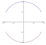
Figure 1. Graph of $\text{\rm{supp}}(d\mu)$

The measure $d\mu_{y}$ is supported on two arcs, $[\theta_{y},\pi-\theta_{y}]$ and $[\pi+\theta_{y},2\pi-\theta_{y}]$, with a.c. part

$$w_{y}(\theta)=w_{y}(\theta)|_{[\theta_{y},\pi-\theta_{y}]}+w_{y}(\theta)|_{[\pi+\theta_{y},2\pi-\theta_{y}]}$$ (4.4)

where

$$w_{y}(\theta) = 2\pi|\sin(\theta)|f_{y}(2\cos\theta)\chi_{[\theta_{y},\pi-\theta_{y}]}(\theta)$$ (4.5)

$$\theta_{y} = \cos^{-1}\left(\frac{y}{2}\right)\in\left(0,\frac{\pi}{2}\right)$$ (4.6)

By Corollary 13.1.8 of [14], $b_{n}(d\gamma_{y})\equiv 0$ if and only if $\alpha_{2n}(d\mu_{y})\equiv 0$. Therefore, we can express the Verblunsky coefficients of $d\mu_{y}$ as

$$0,\tau_{0},0,\tau_{1},0,\tau_{2},\dots$$ (4.7)

with $\tau_{j}=\alpha_{2j+1}$. Moreover, by Theorem 13.1.7 of [14], we know that

$$\begin{array}[]{ll}a_{n+1}^{2}(d\gamma_{y})&=(1-\alpha_{2n-1}(d\mu_{y}))(1-\alpha_{2n}(d\mu_{y})^{2})(1+\alpha_{2n+1}(d\mu_{y}))\\ &=(1-\tau_{n-1})(1+\tau_{n})\end{array}$$ (4.8)

Now we will choose a suitable family of $\tau_{n}\in\mathbb{R}$ such that the corresponding $a_{n}(d\gamma_{y})$ satisfy both (3.1) and (4.8).

Observe that by (4.8) above,

$$a_{n+1}(d\gamma_{y})^{2}-a_{n}(d\gamma_{y})^{2}=(1-\tau_{n-1})(\tau_{n}-\tau_{n-1})+(1+\tau_{n-1})(\tau_{n-1}-\tau_{n-2})$$ (4.9)

Therefore, if we have an increasing family of $\tau_{n}<0$ such that

$$\tau_{n}\nearrow\tau_{\infty}=-\sqrt{1-\left(\displaystyle\frac{y}{2}\right)^{2}}<0$$ (4.10)

then $a_{n}(d\gamma_{y})\nearrow y/2$ and the corresponding measure $d\mu_{y}$.

In particular, if we let

$$\tau_{k}=\displaystyle\tau_{\infty}-\frac{1}{\sqrt{k}}$$ (4.11)

then the goal is achieved.

Next, we prove the following lemma:

Lemma 4.1.

Let $d\mu_{y}$ be the measure on $\partial\mathbb{D}$ with Verblunsky coefficients as in (4.7) where for all large $n$,

$$\tau_{n}=\tau_{\infty}-\displaystyle\frac{1}{\sqrt{n}}\quad\quad-1<\tau_{\infty}<0$$ (4.12)

We add a pure point at $z=1$ to $d\mu_{y}$ as in (2.7) to form $d\tilde{\mu}_{y}$. Then for $n=2m$ or $2m+1$, $\Delta_{n}(1)$ has the following expansion

$$\Delta_{n}(1)=-\tau_{\infty}+\frac{1}{\sqrt{m}}+0+\left(1+\displaystyle\frac{1}{2\tau_{\infty}}\right)\displaystyle\frac{1}{m^{3/2}}+o\left(\displaystyle\frac{1}{m^{3/2}}\right)$$ (4.13)

Therefore,

$$\alpha_{n}(d\mu_{y})=\begin{cases}-\tau_{m}+\displaystyle\left(1+\frac{1}{2\tau_{\infty}}\right)\displaystyle\frac{1}{m^{3/2}}+e_{m}&n=2m\\ \displaystyle\left(1+\frac{1}{2\tau_{\infty}}\right)\displaystyle\frac{1}{m^{3/2}}+e_{m}&n=2m+1\end{cases}$$ (4.14)

where $e_{m}=o\left(m^{-3/2}\right)$.

Proof.

Since all the Verblunsky coefficients of $d\mu_{y}$ are real, by induction on the recursion relation (1.4),

$$\begin{array}[]{ll}\varphi_{n}(1)&=\displaystyle\prod_{j=0}^{n-1}\sqrt{\displaystyle\frac{1-\alpha_{j}}{1+\alpha_{j}}}\end{array}$$ (4.15)

By (4.7), when $n=2m$ or $2m+1$,

$$\varphi_{n}^{*}(1)=\varphi_{n}(1)=\displaystyle\prod_{j=0}^{m-1}\sqrt{\displaystyle\frac{1-\tau_{j}}{1+\tau_{j}}}$$ (4.16)

This formula will play a crucial role in the computation below.

4.1. n is even

First, we compute $\Delta_{n}(1)$ when $n=2m$ using the point mass formula (2.12). Let

$$A_{n} = \overline{\varphi_{n+1}(1)}\varphi_{n}^{*}(1)$$ (4.17)

$$B_{n} = (1-\gamma)\gamma^{-1}+K_{n}(1,1)$$ (4.18)

Then

$$\lim_{m\to\infty}\Delta_{2m}(1)=\lim_{m\to\infty}(1-|\alpha_{2m}|^{2})^{1/2}\,\displaystyle\frac{A_{2m}}{B_{2m}}=\lim_{m\to\infty}\displaystyle\frac{A_{2m}}{B_{2m}}$$ (4.19)

because $\alpha_{2m}=0$ for all $m$. However, instead of computing this directly, we use the Stolz–Cesàro theorem (see [7]), which reads as follows

Theorem 4.1 (Stolz–Cesàro [7]).

Let $(\Gamma_{k})_{k},(\Theta_{k})_{k}$ be two sequences of numbers such that $\Theta_{n}$ is positive, strictly increasing and tends to infinity. If the following limit exists,

$$\lim_{k\to\infty}\frac{\Gamma_{k}-\Gamma_{k-1}}{\Theta_{k}-\Theta_{k-1}}$$ (4.20)

then it is equal to $\lim_{k\to\infty}\Gamma_{k}/\Theta_{k}$.

First, note that $\tau_{k}\to\tau_{\infty}<0$. Thus,

$$B_{m}\approx K_{n}(1,1)>|\varphi_{n}(1)|^{2}\to\infty$$ (4.21)

by (4.16). Hence, it is legitimate for us to use Theorem 4.1 above.

Let $K_{n}\equiv K_{n}(1,1)$ and $\varphi_{n}\equiv\varphi_{n}(1)$. Observe that $\varphi_{2m+1}=\varphi_{2m}$. Therefore, by (4.16),

$$B_{2(m+1)}-B_{2m}=\varphi_{2(m+1)}^{2}+\varphi_{2m}^{2}=\displaystyle\frac{2\varphi_{2m}^{2}}{1+\tau_{m}}$$ (4.22)

and

$$A_{2(m+1)}-A_{2m}=\varphi_{2(m+1)}^{2}-\varphi_{2m}^{2}=\left(\displaystyle\frac{-2\tau_{m}}{1+\tau_{m}}\right)\varphi_{2m}^{2}$$ (4.23)

As a result,

$$\lim_{m\to\infty}\Delta_{2m}(1)=\displaystyle\lim_{m\to\infty}\frac{A_{2(m+1)}-A_{2m}}{B_{2(m+1)}-B_{2m}}=-\tau_{\infty}$$ (4.24)

Next, we will prove that the rate of convergence is

$$\Delta_{2m}(1)=-\tau_{\infty}+\displaystyle\frac{1}{\sqrt{m}}+o\left(\displaystyle\frac{1}{\sqrt{m}}\right)$$ (4.25)

by computing the following limit

$$\lim_{m\to\infty}m\left({\Delta_{2m}(1)+\tau_{\infty}}\right)=1$$ (4.26)

Recall the definition of $\Delta_{n}(1)$ and the facts $\alpha_{2m}\equiv 0$ and $\varphi_{2m+1}\varphi_{2m}=\varphi_{2m}^{2}$. Thus, the left hand side of (4.26) can be expressed as $X_{n}/Y_{n}$, where

$$X_{m} = \sqrt{m}\left[\varphi_{2m}^{2}+\tau_{\infty}K_{2m}\right]$$ (4.27)

$$Y_{m} = K_{2m}\to\infty$$ (4.28)

We use the Stolz–Cesàro Theorem again. First, observe that

$$Y_{m+1}-Y_{m}=\displaystyle\frac{1-\tau_{m}}{1+\tau_{m}}+1=\displaystyle\frac{2}{1+\tau_{m}}\varphi_{2m}^{2}$$ (4.29)

Then we compute

$$X_{2(m+1)}-X_{2m}\\ =\underbrace{\left[\sqrt{m+1}\displaystyle\frac{1-\tau_{m}}{1+\tau_{m}}-\sqrt{m}\right]\varphi_{2m}^{2}}_{\text{(I)}}+\underbrace{\tau_{\infty}\left[\sqrt{m+1}K_{2(m+1)}-\sqrt{m}K_{2m}\right]}_{\text{(II)}}$$ (4.30)

Consider each term in (4.30) above.

$$\frac{\text{(I)}}{Y_{2(m+1)}-Y_{2m}}=\displaystyle\frac{\sqrt{m+1}\frac{1-\tau_{m}}{1+\tau_{m}}-\sqrt{m}}{\frac{2}{1+\tau_{m}}}=\displaystyle\frac{\sqrt{m+1}(1-\tau_{m})-\sqrt{m}(1+\tau_{m})}{2}$$ (4.31)

Moreover,

$$\text{(II)}=\tau_{\infty}\left[\sqrt{m+1}(K_{2(m+1)}-K_{2m})+(\sqrt{m+1}-\sqrt{m})K_{2m}\right]$$ (4.32)

which implies that

$$\frac{\text{(II)}}{Y_{m+1}-Y_{m}}=\tau_{\infty}\left[\sqrt{m+1}+(\sqrt{m+1}-\sqrt{m})\displaystyle\frac{1+\tau_{m}}{2}\frac{K_{2m}}{\varphi_{2m}^{2}}\right]$$ (4.33)

Next, we show that $\lim_{m\to\infty}K_{2m}/\varphi_{2m}^{2}=-1/\tau_{\infty}$ by the Stolz–Cesàro Theorem.

$$\begin{array}[]{ll}\displaystyle\lim_{m\to\infty}\frac{K_{2m}}{\varphi_{2m}^{2}}&=\left(\displaystyle\lim_{m\to\infty}\displaystyle\frac{\varphi_{2(m+1)}^{2}-\varphi_{2m}^{2}}{K_{2(m+1)}-K_{2m}}\right)^{-1}\\ &=\displaystyle\lim_{m\to\infty}\displaystyle\left({\frac{1-\tau_{m}}{1+\tau_{m}}-1}\right)^{-1}\left({\frac{1-\tau_{m}}{1+\tau_{m}}+1}\right)\\ &=-\displaystyle\frac{1}{\tau_{\infty}}\end{array}$$ (4.34)

Combining (4.31), (4.33) and (4.34), we obtain

$$\lim_{m\to\infty}m\left({\Delta_{2m}(1)-(\tau_{\infty})}\right)=1$$ (4.35)

Next, we are going to show that

$$\Delta_{2m}(1)=-\tau_{\infty}+\displaystyle\frac{1}{\sqrt{m}}+o\left(\displaystyle\frac{1}{m}\right)$$ (4.36)

by computing the second-order term. We do so by proving that

$$L_{2}\equiv\displaystyle\lim_{m\to\infty}m\left(\Delta_{2m}-(-\displaystyle\tau_{\infty})-\displaystyle\frac{1}{\sqrt{m}}\right)=0$$ (4.37)

Let

$$P_{m}=m\varphi_{2m}^{2}+m\tau_{\infty}K_{2m}-\sqrt{m}K_{2m}$$ (4.38)

Then

$$P_{m+1}-P_{m}=\left[(m+1)\displaystyle\frac{1-\tau_{m}}{1+\tau_{m}}-m\right]\varphi_{2m}^{2}\\ +(m+1)\tau_{\infty}\left[K_{2(m+1)}-K_{2m}\right]+\left[(m+1)-m\right]\tau_{\infty}K_{2m}\\ -\sqrt{m+1}\left[K_{2(m+1)}-K_{2m}\right]-(\sqrt{m+1}-\sqrt{m})K_{2m}$$ (4.39)

Combining with previous results about $Y_{m+1}-Y_{m}$ and $K_{2m}/\varphi_{2m}^{2}$, we have

$$L_{2}=\displaystyle\lim_{m\to\infty}\frac{P_{m+1}-P_{m}}{Y_{m+1}-Y_{m}}=0$$ (4.40)

which proves (4.36).

Next, we will obtain the third-order term by computing

$$L_{3}=\displaystyle\lim_{m\to\infty}m^{3/2}\left(\Delta_{2m}-(-\tau_{\infty})-\displaystyle\frac{1}{\sqrt{m}}\right)$$ (4.41)

Let

$$J_{m}=m^{3/2}\varphi_{2m}^{2}+m^{3/2}\tau_{\infty}K_{2m}-mK_{2m}$$ (4.42)

By a similar argument as in (4.34),

$$J_{m+1}-J_{m}=\left[(m+1)^{3/2}\displaystyle\frac{1-\tau_{m}}{1+\tau_{m}}-m^{3/2}\right]\varphi_{2m}^{2}\\ +(m+1)^{3/2}\tau_{\infty}\left[K_{2(m+1)}-K_{2m}\right]+\left[(m+1)^{3/2}-m^{3/2}\right]\tau_{\infty}K_{2m}\\ -(m+1)\left[K_{2(m+1)}-K_{2m}\right]-(m+1-m)K_{2m}$$ (4.43)

which implies that

$$L_{3}=\displaystyle\lim_{m\to\infty}\displaystyle\frac{J_{m}}{Y_{m}}=1+\frac{1}{2\tau_{\infty}}$$ (4.44)

4.2. when n is odd

We compute $\Delta_{n}(1)$ when $n=2m+1$ using the point mass formula (2.12). Let $A_{n}$ and $B_{n}$ be defined as in (4.17) and (4.18). Then

$$\lim_{m\to\infty}\Delta_{2m+1}(1)=(1-|\tau_{\infty}|^{2})^{1/2}\lim_{m\to\infty}\,\displaystyle\frac{A_{2m+1}}{B_{2m+1}}$$ (4.45)

We will use the Stolz–Cesàro Theorem again. Note that

$$A_{2(m+1)+1}-A_{2m+1}=\left(\displaystyle\sqrt{\frac{1-\tau_{m+1}}{1+\tau_{m+1}}}\frac{1-\tau_{m}}{1+\tau_{m}}-\displaystyle\sqrt{\frac{1-\tau_{m}}{1+\tau_{m}}}\right)\varphi_{2m}^{2}$$ (4.46)

and because $\varphi_{2m+3}=\varphi_{2m+2}$,

$$B_{2(m+1)+1}-B_{2m+1}=2\varphi_{2m+2}^{2}=2\left(\frac{1-\tau_{m}}{1+\tau_{m}}\right)\varphi_{2m}^{2}$$ (4.47)

Therefore,

$$\lim_{m\to\infty}\Delta_{2m+1}(1)=\displaystyle\frac{-\tau_{\infty}(1-|\tau_{\infty}|^{2})^{1/2}}{\sqrt{(1+\tau_{\infty})(1-\tau_{\infty})}}=-\tau_{\infty}$$ (4.48)

Next, we prove the rate of convergence by computing

$$\lim_{m\to\infty}\sqrt{m}\left({\Delta_{2m+1}(1)+\tau_{\infty}}\right)=1$$ (4.49)

Since $\alpha_{n}\in\mathbb{R}$, the recursion relation becomes

$$(1-|\alpha_{n}|^{2})^{1/2}\varphi_{n+1}=\varphi_{n}-\overline{\alpha_{n}}\varphi_{n}^{*}=(1-\alpha_{n})\varphi_{n}$$ (4.50)

Therefore,

$$\Delta_{2m+1}(1)=\displaystyle\frac{(1-\alpha_{2m+1})\varphi_{2m+1}^{2}}{K_{2m+1}}=(1-\tau_{m})\displaystyle\frac{\varphi_{2m}^{2}}{K_{2m+1}}$$ (4.51)

Let

$$P_{m} = \sqrt{m}\left[(1-\tau_{m})\varphi_{2m}^{2}+\tau_{\infty}K_{2m+1}\right]$$ (4.52)

$$Q_{m} = K_{2m+1}\to\infty$$ (4.53)

Note that

$$Q_{m+1}-Q_{m}=K_{2m+3}-K_{2m+1}=2\varphi_{2(m+1)}^{2}$$ (4.54)

and

$$P_{m+1}-P_{m}=\underbrace{\left[\sqrt{m+1}(1-\tau_{m+1})\varphi_{2(m+1)}^{2}-\sqrt{m}(1-\tau_{m})\varphi_{2m}^{2}\right]}_{\text{(I)}}\\ +\tau_{\infty}\sqrt{m+1}\left[K_{2m+3}-K_{2m+1}\right]+\underbrace{(\sqrt{m+1}-\sqrt{m})\tau_{\infty}K_{2m+1}}_{\text{(II)}}$$ (4.55)

Since $(1-\tau_{m})\varphi_{2m}^{2}=(1+\tau_{m})\varphi_{2(m+1)}^{2}$,

$$\begin{array}[]{ll}\displaystyle\frac{\text{(I)}}{Q_{m+1}-Q_{m}}&=\displaystyle\frac{\sqrt{m+1}(1-\tau_{m+1})-\sqrt{m}(1+\tau_{m})}{2}\end{array}$$ (4.56)

Next, consider (II). We compute

$$\lim_{m\to\infty}\displaystyle\frac{\varphi_{2(m+1)}^{2}-\varphi_{2m}^{2}}{K_{2m+1}-K_{2m-1}}=\displaystyle\frac{\left(\frac{1-\tau_{m}}{1+\tau_{m}}-1\right)\varphi_{2m}^{2}}{2\varphi_{2m}^{2}}=\displaystyle\frac{-\tau_{\infty}}{1+\tau_{\infty}}$$ (4.57)

which implies

$$\frac{\text{(II)}}{Q_{m+1}-Q_{m}}=-(1+\tau_{\infty})(\sqrt{m+1}-\sqrt{m})$$ (4.58)

Therefore,

$$\lim_{m\to\infty}m\left(\Delta_{2m+1}(1)-(-\tau_{\infty})\right)=\displaystyle\lim_{m\to\infty}\frac{P_{m}}{Q_{m}}=1$$ (4.59)

Next, we will prove that

$$\Delta_{2m+1}=-\tau_{\infty}+\displaystyle\frac{1}{\sqrt{m}}+o\left(\displaystyle\frac{1}{m}\right)$$ (4.60)

by showing

$$L_{2}^{\prime}\equiv\displaystyle\lim_{m\to\infty}m\left(\Delta_{2m+1}+\tau_{\infty}-\frac{1}{\sqrt{m}}\right)=0$$ (4.61)

As explained in (4.51), it suffices to consider

$$H_{m}=m(1-\tau_{m})\varphi_{2m}^{2}+m\tau_{\infty}K_{2m+1}-\sqrt{m}K_{2m+1}$$ (4.62)

$$H_{m+1}-H_{m}=\underbrace{(m+1)(1-\tau_{m+1})\varphi_{2(m+1)}^{2}-m(1-\tau_{m})\varphi_{2m}^{2}}_{\text{(I)}}\\ \underbrace{+(m+1)\tau_{\infty}K_{2m+3}-m\tau_{\infty}K_{2m+1}}_{\text{(II)}}\underbrace{-\sqrt{m+1}K_{2m+3}+\sqrt{m}K_{2m+1}}_{\text{(III)}}$$ (4.63)

Since $(1-\tau_{m})\varphi_{2m}^{2}=(1+\tau_{m})\varphi_{2(m+1)}^{2}$, we have

$$\frac{\text{(I)}}{Q_{m+1}-Q_{m}}=\displaystyle\frac{(m+1)(1-\tau_{m+1})-m(1+\tau_{m})}{2}$$ (4.64)

$$\frac{\text{(II)}}{Q_{m+1}-Q_{m}}=\tau_{\infty}(m+1)+(m+1-m)\tau_{\infty}\displaystyle\frac{K_{2m+1}}{2\varphi_{2(m+1)}^{2}}$$ (4.65)

$$\frac{\text{(III)}}{Q_{m+1}-Q_{m}}=\displaystyle\frac{(-\sqrt{m+1}+\sqrt{m})K_{2m+3}}{2\varphi_{2(m+1)}^{2}}+(-\sqrt{m})$$ (4.66)

This proves that $L^{\prime}=0$ and thus (4.60).

Next, we compute

$$L_{3}^{\prime}=\displaystyle\lim_{m\to\infty}m^{3/2}\left(\Delta_{2m+1}+\tau_{\infty}-\displaystyle\frac{1}{\sqrt{m}}\right)$$ (4.67)

By similar arguments as in (4.64), (4.65) and (4.66), we conclude that

$$L_{3}^{\prime}=1+\displaystyle\frac{1}{2\tau_{\infty}}$$ (4.68)

This concludes the proof of Lemma 4.1 ∎

Finally, we apply the Szegő map to this perturbed measure $d\tilde{\mu}_{y}$ to form the perturbed measure $d\tilde{\gamma}_{y}$ on $[-2,2]$, which is defined by

$$\tilde{\gamma}_{y}(x)=(1-\gamma)d\gamma_{y}(x)+\gamma\delta_{x=2}$$ (4.69)

For the sake of convenience, we temporarily denote $\alpha_{n}\equiv\alpha_{n}(d\tilde{\mu}_{y})$. Since $b_{n}(d\gamma_{y})\equiv 0$, if suffices to consider

$$b_{n+1}(d\gamma_{y})=\displaystyle\frac{1}{\sqrt{n}}-\displaystyle\frac{1}{\sqrt{n-1}}+o\left(\displaystyle\frac{1}{n^{3/2}}\right)=\frac{-1}{2n^{3/2}}+o\left(\frac{1}{n^{3/2}}\right)$$ (4.70)

It is more complicated with $a_{n}(d\tilde{\gamma_{y}})$. Recall that

$$a_{n+1}(d\tilde{\gamma}_{y})^{2}=(1-\alpha_{2n-1})(1-\alpha_{2n}^{2})(1+\alpha_{2n+1})\\$$ (4.71)

and we know that

$$a_{n+1}(d\gamma_{y})^{2}=(1-\tau_{n-1})(1+\tau_{n})$$ (4.72)

Therefore, upon solving the algebra, we obtain

$$a_{n+1}(d\tilde{\gamma}_{y})^{2}-a_{n+1}(d\gamma_{y})^{2}=\displaystyle\frac{1}{2(1+\tau_{\infty})m^{3/2}}+o\left(\displaystyle\frac{1}{m^{3/2}}\right)$$ (4.73)

Upon scaling, we have

$$a_{n+1}^{2}(d{\gamma})-a_{n+1}^{2}(d\gamma_{0})=\displaystyle\frac{2}{y^{2}(1+\tau_{\infty})m^{3/2}}+o\left(\displaystyle\frac{1}{m^{3/2}}\right)$$ (4.74)

5. acknowledgement

I would like to thank Professor Barry Simon for suggesting this problem and for all the very helpful discussions.

References

[1] G. Borg, Eine Umkehrung der Sturm-Liouvilleschen Eigenwertaufgabe. Bestimmung der Differentialgleichung durch die Eigenwerte,
Acta Math. 78 (1946), 1–96.
[2] A. Cachafeiro and F. Marcellán, Asymptotics for the ratio of the leading coefficients of orthogonal polynomials associated with a jump modification, in ”Approximation and Optimization” (Havana, 1987), 111–117, Lecture Notes in Math., 1354, Springer, Berlin, 1988.
[3] A. Cachafeiro and F. Marcellán, Orthogonal polynomials and jump modifications, in ”Orthogonal Polynomials and Their Applications”, (Segovia, 1986), pp. 236–240, Lecture Notes in Math., 1329, Springer, Berlin, 1988.
[4] A. Cachafeiro and F. Marcellán, Perturbations in Toeplitz matrices, in Orthogonal Polynomials and Their Applications , (Laredo, 1987), pp. 139–146, Lecture Notes in Pure and Applied Math., 117, Marcel Dekker, New York, 1989.
[5] A. Cachafeiro and F. Marcellán, Perturbations in Toeplitz matrices: Asymptotic properties, J. Math. Anal. Appl. 156 (1991) 44–51.
[6] A. Cachafeiro and F. Marcellán, Modifications of Toeplitz matrices: jump functions, Rocky Mountain J. Math. 23 (1993), 521–531.
[7] E. Cesàro and O. Stolz, http://en.wikipedia.org/wiki/Stolz-Cesàro_theorem.
[8] I. M. Gel’fand and B. M. Levitan, On the determination of a differential equation from its spectral function, Amer. Math. Soc. Transl. (2) 1 (1955), 253–304; Russian original in Izvestiya Akad. Nauk SSSR. Ser. Mat. 15 (1951), 309–360.
[9] Ya. L. Geronimus, On the trigonometric moment problem, Ann. of Math. (2) 47 (1946), 742–761.
[10] Ya. L. Geronimus, Polynomials Orthogonal on a Circle and Their Applications, Amer. Math. Soc. Translation 1954 (1954), no. 104, 79pp.
[11] Ya. L. Geronimus, Orthogonal Polynomials: Estimates, Asymptotic Formulas, and Series of Polynomials Orthogonal on the Unit Circle and on an Interval, Consultants Bureau, New York, 1961.
[12] P. Nevai, Orthogonal polynomials, measures and recursions on the unit circle, Trans. Amer. Math. Soc. 300 (1987), 175–189.