Simplified Hydrostatic Carbon Burning in White Dwarf Interiors.

Abstract

We introduce two simplified nuclear networks that can be used in hydrostatic carbon burning reactions occurring in white dwarf interiors. They model the relevant nuclear reactions in carbon–oxygen white dwarfs (CO WDs) approaching ignition in Type Ia supernova (SN Ia) progenitors, including the effects of the main $e^{-}$–captures and $\beta$–decays that drive the convective Urca process. They are based on studies of a detailed nuclear network compiled by the authors and are defined by approximate sets of differential equations whose derivations are included in the text. The first network, N1, provides a good first order estimation of the distribution of ashes and it also provides a simple picture of the main reactions occuring during this phase of evolution. The second network, N2, is a more refined version of N1 and can reproduce the evolution of the main physical properties of the full network to the 5% level. We compare the evolution of the mole fraction of the relevant nuclei, the neutron excess, the photon energy generation and the neutrino losses between both simplified networks and the detailed reaction network in a fixed temperature and density parcel of gas.

1 INTRODUCTION

Type Ia supernovae (SNe Ia) are the thermonuclear explosions of white dwarf stars. They are observable end–points of stellar evolution, they shape the energy and chemistry evolution of galaxies and have been successfully used as distance indicators up to redshifts of $\sim 1.7$ thanks to an empirical decline rate – luminosity relation (Pskovskii, 1977; Phillips, 1993). This relationship led to the discovery of the acceleration of the Universe (Riess et al., 1998; Perlmutter et al., 1999)

The exact nature of SN Ia progenitors is still debated (Hillebrandt & Niemeyer, 2000), but most models involve an accreting carbon–oxygen white dwarf (CO WDs) with a mass close to the Chandrasekhar mass (Nomoto, Thielemann, & Yokoi, 1984). This CO WD would accrete mass from either a slightly evolved main sequence companion (CO WD + MS), a more evolved red giant star (CO WD + RG), or a Helium star (CO WD + He), in the so–called single degenerate scenarios (SD, see e.g. Hachisu, Kato, & Nomoto, 1996; Li & van den Heuvel, 1997; Hachisu, Kato, & Nomoto, 1999; Hachisu, Kato, Nomoto, & Umeda, 1999; Langer, Deutschmann, Wellstein, Hoeflich, 2000; Han & Podsiadlowski, 2004; Meng, Chen, & Han, 2009), or as a result of the merger of two degenerate stars with a combined mass above the Chandrasekhar limit, in the double degenerate scenario (DD, see e.g. Webbink, 1984; Iben & Tutukov, 1984). It has been suggested that only CO WDs accreting within a narrow range lead to successful thermonuclear explosions (see e.g. Nomoto & Kondo, 1991; Nomoto, Saio, Kato, & Hachisu, 2007), unless additional physical processes are included in the models, e.g. rotation and other three–dimensional effects (see e.g. Domínguez et al., 2006; Yoon, Podsiadlowski, & Rosswog, 2007; Pakmor et al., 2010).

The diversity of SN Ia ejecta and the origin of the decline rate–absolute magnitude relation are being understood only recently thanks to new observational techniques and energy transfer codes (see e.g. Mazzali, Röpke, Benetti, & Hillebrandt, 2007; Woosley, Kasen, Blinnikov, & Sorokina, 2007; Kromer & Sim, 2009). These efforts have been accompanied by new developments in the physics of the explosion which have shown that even if pure deflagration models can reproduce many SN Ia spectra and light curves (Röpke et al., 2007), in some cases a delayed detonation may be necessary (Khokhlov, 1991; Röpke et al., 2007). The physics of both the transition to detonation and ignition of the deflagration wave remain uncertain (Iapichino, Brüggen, Hillebrandt, & Niemeyer, 2006; Röpke, 2007; Iapichino & Lesaffre, 2010).

A related problem, rarely addressed in the literature, is how to connect theoretical models with observed systematic differences between SNe Ia occurring in different stellar environments (e.g. Hamuy et al., 1996; Sullivan et al., 2006). These should be related to the pre–supernova evolution and not to line–of–sight effects or other processes occuring randomly during the explosion (e.g. Kasen, Röpke, & Woosley, 2009; Maeda et al., 2010). Thus, presupernova evolution must play a significant role in the diversity of SN Ia explosions (Lesaffre et al., 2006).

1.1 Presupernova Evolution: from Cooling to Ignition

Here we will assume that the progenitors of SNe Ia originate in the SD scenario; but note that, even in the standard DD scenario, the core would evolve in a very similar way in the immediate pre-explosion phase (i.e. during the last $\sim 10^{3}\,$yr; see Yoon, Podsiadlowski, & Rosswog, 2007).

Before a SN Ia progenitor becomes unbound by the explosion it undergoes several distinct phases of evolution (Nomoto, Thielemann, & Yokoi, 1984; Lesaffre et al., 2006). First, the progenitor white dwarf cools down at almost constant density after its birth, for a period of hundreds or thousands of Myr, depending on the particular formation scenario (the cooling phase). Then, it accretes matter for a period of the order of one Myr, making the degenerate star shrink to keep the hydrostatic equilibrium and its core compress adiabatically, the accretion phase. Adiabatic compression at the center and heat diffusion from the hot accreting envelope can make the central temperature increase under degenerate conditions, triggering hydrostatic carbon burning and a new source of energy generation. The energy input from hydrostatic carbon burning will force the star to transport the excess energy at its center convectively, the simmering phase. During this phase the convective core can grow to engulf most of the star. If the central density is high enough, $e^{-}$–captures and $\beta$–decays can become important. In the presence of a convective core, that process has been called the convective Urca process.

At some point energy deposition will dominate over the energy losses, making the star’s central temperature increase at almost constant density, the thermonuclear flash. Finally, when the temperature is high enough, one or more ignition spots will give rise to nuclear flames that will propagate in the highly convective medium, the thermonuclear runaway, causing a deflagration wave to sweep over the star, sometimes transitioning into a detonation wave. The deflagration and detonation waves will generate most of the kinetic energy and ashes in the ejecta in a few seconds, including radioactive matter which will later power the light curve of the supernova. Since this last phase will occur at very high temperatures, the characteristic burning time–scales will be much shorter than the typical weak interaction time–scales and the neutron excess of the ejecta will not differ from that of the presupernova star, except for the star’s innermost regions where weak interaction time–scales are shorter. Most of the WD’s neutron excess changes will occur before ignition.

1.2 Nuclear physics and the convective URCA process

One of the main obstacles that remain to be solved in order to obtain self–consistent pre–supernova models up to ignition is the convective Urca process, which was mentioned in the previous section. The following factors make this phase of evolution difficult to solve: (1) the appearance of a fast–growing convective core with a very steep luminosity and composition gradient at its outer edge, the so–called C–flash; (2) a high–density medium with $e^{-}$–capture and $\beta$–decay time–scales similar to the convective time–scales, which have an uncertain effect over the energy budget of the star; (3) a steep density gradient which changes rapidly when the WD approaches the Chandrasekhar mass; (4) a steep composition gradient of the Urca pair ${}^{23}{\rm Na}$–${}^{23}{\rm Ne}$ at the threshold density for electron captures, which moves inwards as the central density increases and (5) an increasingly complex set of nuclear reactions as carbon burns and pollutes the WD with its ashes, with a time–scale that can be similar to $e^{-}$–capture and $\beta$–decay time–scales

It is not clear whether $e^{-}$–captures and $\beta$–decays of Urca matter around a threshold density in a convective medium have a cooling or heating effect over time. Many studies over the years have reached different conclusions regarding this point. Paczyński (1972) first suggested that Urca processes have a stabilizing effect over carbon burning, leading to the formation of a neutron star instead of a thermonuclear explosion. Bruenn (1973) realized that $e^{-}$–captures can cause heating by creating holes in the Fermi sea, which dominate over the neutrino losses for the most important Urca pairs. Couch & Arnett (1974) found that significant work must be done to mantain convection when Urca processes occur, with a net cooling effect, but Regev & Shaviv (1975) pointed out that convection cannot develop fast enough to prevent heating. Barkat & Wheeler (1990) summarized the factors controlling the Urca process, but it was later shown that the role of the kinetic energy flux should have been included in their analysis (Mochkovitch, 1996; Stein et al., 1999). More recently, Lesaffre, Podsiadlowski, & Tout (2005) showed that the heating effect of the Urca process depends on the state of mixing of the convective core, that the convective velocities are reduced by Urca processes and that time–dependent computations with a full nuclear network are needed to understand the effect of Urca processes on the ignition conditions of SNe Ia.

In this study we have focused on how to accurately treat the increasingly complex nuclear reactions as the WD is polluted with ashes. We do not attempt to answer whether Urca processes cause cooling or heating, but provide a tool for better evaluating the competing heating and cooling mechanisms in a presupernova WD approaching ignition.

In what follows we will introduce two approximations that use a limited number of nuclei to accurately describe the evolution of the main species that result from the burning of ${}^{12}{\rm C}$, the energy deposition rate, the energy losses via neutrinos and the neutron excess. We will show when these approximations hold, and their potential applications, but first we will introduce a detailed nuclear network which will be used for comparison with the simplified networks.

2 THE FULL NUCLEAR NETWORK

Figure 1: Ratio between the two main carbon burning reactions (thermally averaged cross–sections) plotted against the temperature in $10^{9}$ K.

The nuclear reactions within a CO WD approaching explosion are characterized by the burning of ${}^{12}{\rm C}$ nuclei at high densities ($>10^{7}$ g cm^-3) and high temperatures ($>10^{8}$ K) in an environment rich in ${}^{12}{\rm C}$ and ${}^{16}{\rm O}$ nuclei and relatively devoid of free protons, $\alpha$–particles or neutrons. The dominant reactions are $\rm{{}^{12}C(^{12}C,p)^{23}Na}$, Q = 4.6 MeV, and $\rm{{}^{12}C(^{12}C,^{4}He)^{20}Ne}$, Q = 2.2 MeV, both occurring at similar rates (see Figure 1). The nuclear network increases in complexity as the ${}^{12}{\rm C}$–burning pollutes the WD with its ashes, mainly ${}^{20}{\rm Ne}$ and ${}^{23}{\rm Na}$, but also with protons and $\alpha$–particles, which will be processed into additional ${}^{16}{\rm O}$ and ${}^{13}{\rm C}$ nuclei, as will be shown later.

We have integrated a detailed reaction network at fixed temperature and density compiled by the authors. The system of differential equations defining the network is solved for using the semi–implicit extrapolation method from Bader & Deuflhard (1983). We include species that are part of the reactions known to be most important, or those close to them in a table of nuclides. We include all reaction rates between species of our network that are either in the Reaclib library (Thielemann et al., 2006), or in the weak interaction tables by Oda et al. (1994), as well as improved ${}^{13}{\rm N}(e^{-},\nu_{e})^{13}{\rm C}$ rates from Zegers et al. (2008). Screening corrections were also included under the simplification of Graboske, Dewitt, Grossman, & Cooper (1973). Recent formalisms that treat carbon burning and screening corrections in alternative ways were not implemented for this work (see e.g. Gasques et al., 2005; Yakovlev et al., 2006; Spillane et al., 2007).

We have assumed that the initial C/O ratio is always given by the nuclide mass fractions X(${}^{12}{\rm C}$) = 0.3 and X(${}^{16}{\rm O}$) = 0.7, in order to compare with the work by Chamulak, Brown, Timmes, & Dupczak (2008), but reasonable variations of the initial compositions do not affect the validity of our approximations.

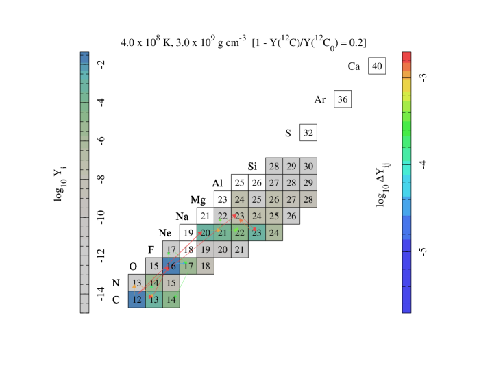
Figure 2: Main flows at a temperature of 4$\times 10^{8}$K and densities of 1$\times 10^{9}$ g cm^-3 (top) and 3$\times 10^{9}$ g cm^-3 (bottom) when 20% of the original carbon has been burnt.

Figure 2 show the main flows in our nuclear network at a temperature of $3\times 10^{8}$ K and densities of $1\times 10^{9}$ g cm^-3 (top) and $3\times 10^{9}$ g cm^-3 (bottom), starting from a pure carbon–oxygen mixture, when 20% of the original carbon nuclei have been burnt. The left hand side color–coding bar indicates the mole fraction scale of the individual species, whereas the right hand side color–coding bar indicates the mole fraction flow scale of the individual reactions. Only reactions that are bigger than one thousandth of the biggest flow are plotted.

The main differences between the low density (top) and high density (bottom) flow diagrams are due to $e^{-}$–captures in the ²³Na(e^-, $\nu_{e}$)²³Ne reaction, which only occurs at densities higher than $\sim$1.7$\times 10^{9}$ g cm^-3. Below this density the $e^{-}$–captures are almost exclusively due to the ${}^{13}{\rm N}(e^{-},\nu_{e})^{13}{\rm C}$ reaction.

The advantage of this detailed network is that it can accurately track the evolution of nuclei with a wide range of characteristic time–scales. For example, it is capable of accurately following the mole fraction of $\alpha$–particles, protons, neutrons or fast electron–capturing ${}^{13}{\rm N}$ nuclei, as well as long characteristic time–scale nuclei like ${}^{12}{\rm C}$, or intermediate time–scale nuclei like ${}^{23}{\rm Na}$ at high densities.

Since we study this reaction network in convective WD interiors, we must consider the relation between the relevant burning time–scales and the convective turn–over time–scale, which is determined by the diffusion time–scale and the temperature, density and composition gradients of the star. The convective time–scale will be the shortest time–scale that affects the evolution of the structure of the star that is not directly connected to the nuclear physics, and can be as low as 50 sec before ignition (see Figure 6 in Lesaffre et al., 2006).

Ideally, we would like to build an approximated nuclear network where we remove time–scales much shorter than the convective time–scale from the resulting set of differential equations, as long as a reasonable physical justification is provided. This would reduce the number of variables per zone while keeping accuracy and would make the inversion of the corresponding Jacobian in a Newton–Raphson integration scheme more stable.

We have found two approximate solutions that achieve the former based on the detailed nuclear network at fixed density and temperature described in this section (see also Chamulak, Brown, Timmes, & Dupczak, 2008; Piro & Bildsten, 2008). The first such approximation will be described in the following section.

3 THE SIMPLIFIED NETWORK: FIRST APPROXIMATION (N1)

To accurately follow the chemistry of the evolving WD progenitor towards explosion, the simultaneous solution of the structure and chemistry of the star is required (Stancliffe, 2006). The chemistry equations must be able to reproduce the evolution of the main species and their effect on the star through changes in energy deposition, energy losses or the electron fraction. This can become computationally demanding if too many species are included and can worsen during the simmering phase of evolution due to known convergence problems (Iben, 1978, 1982), even with approximate theories of convection.

We have found a first order approximation to the full nuclear network which will be described in this section. We will refer to this approximation as N1. A more accurate version of this approximation, N2, will be described in Section 5. Both simplified networks use the fact that the dominant carbon burning reactions, ${}^{12}{\rm C}(^{12}{\rm C},p)^{23}{\rm Na}$ and ${}^{12}{\rm C}(^{12}{\rm C},\alpha)^{20}{\rm Ne}$, occur nearly at the same rate and the abundances of protons, $\alpha$–particles, neutrons and ${}^{13}{\rm N}$ nuclei are approximately at equilibrium most of the time. This can be explained by the complementarity of the relevant reactions (see Figure 3 and 4), which was first noticed by Chamulak, Brown, Timmes, & Dupczak (2008) and Piro & Bildsten (2008).

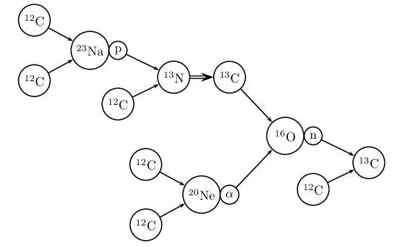
Figure 3: Main ${}^{12}{\rm C}$ burning reactions and its ashes at low density. Six ${}^{12}{\rm C}$ nuclei are consumed to produce four nuclei: ${}^{23}{\rm Na}$, ${}^{20}{\rm Ne}$, ${}^{16}{\rm O}$ and ${}^{13}{\rm C}$ and one electron capture in the reaction ${}^{13}{\rm N}(e^{-},\nu_{e})^{13}{\rm C}$. The figure is shown as a rotated tree, with parent nuclei connected to children nuclei in the direction indicated by the arrows. Double arrows correspond to electron captures or inverse beta decays.

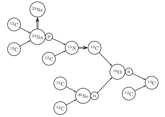
Figure 4: Same as Figure 3, but at high density. Six ${}^{12}{\rm C}$ nuclei are consumed to produce four nuclei: ${}^{23}{\rm Ne}$, ${}^{20}{\rm Ne}$, ${}^{16}{\rm O}$ and ${}^{13}{\rm C}$ and two $e^{-}$–captures in the reactions ${}^{13}{\rm N}(e^{-},\nu_{e})^{13}{\rm C}$ and ${}^{23}{\rm Na}(e^{-},\nu_{e})^{23}{\rm Ne}$.

First, when in the carbon burning reaction ${}^{12}{\rm C}(^{12}{\rm C},p)^{23}{\rm Na}$ a proton is released, it will be captured quickly, preferentially in the ${}^{12}{\rm C}(p,\gamma)^{13}{\rm N}$ reaction. Second, ${}^{13}{\rm N}$ will quickly capture an electron in the ${}^{13}{\rm N}(e^{-},\nu_{e})^{13}{\rm C}$ reaction, decreasing the pressure and lifting the degeneracy of the gas, and producing a ${}^{13}{\rm C}$ nucleus. Third, in the carbon burning reaction ${}^{12}{\rm C}(^{12}{\rm C},\alpha)^{20}{\rm Ne}$ an $\alpha$–particle will be released and quickly captured in the ${}^{13}{\rm C}(\alpha,n)^{16}{\rm O}$ reaction, thus consuming the ${}^{13}{\rm C}$ nucleus just produced, but liberating a neutron. Fourth, the free neutron will be preferentially captured in the ${}^{12}{\rm C}(n,\gamma)^{13}{\rm C}$ reaction, thus recovering the ${}^{13}{\rm C}$ just consumed. Hence, the net effect is approximately the burning of six ${}^{12}{\rm C}$ nuclei and the capture of one electron to be replaced by four nuclei: ${}^{20}{\rm Ne}$, ${}^{23}{\rm Na}$, ${}^{16}{\rm O}$ and ${}^{13}{\rm C}$, i.e.:

$$6~{}^{12}{\rm C}+e^{-}~{}\rightarrow~{}^{23}{\rm Na}~{}+~{}^{20}{\rm Ne}~{}+~{}^{16}{\rm O}~{}+~{}^{13}{\rm C}.$$ (1)

An additional $e^{-}$–capture can occur via the ${}^{23}{\rm Na}(e^{-},\nu_{e})^{23}{\rm Ne}$ reaction if the density is above $\approx 1.7\times 10^{9}$ g cm^-3. In this case, two $e^{-}$–captures can occur and the net effect is:

$$6~{}^{12}{\rm C}+2~{}e^{-}~{}\rightarrow~{}^{23}{\rm Ne}~{}+~{}^{20}{\rm Ne}~{}+~{}^{16}{\rm O}~{}+~{}^{13}{\rm C},$$ (2)

which is schematically shown in Figure 4. If any of the flows above is broken the simplified network will fail and will need a different treatment.

Now, we will assume that the only relevant reactions are:

1)	${}^{12}{\rm C}(^{12}{\rm C},p)^{23}{\rm Na}$,	Q = 2.24 MeV,	2)	${}^{12}{\rm C}(^{12}{\rm C},\alpha)^{20}{\rm Ne}$,	Q = 4.62 MeV
3)	${}^{12}{\rm C}(p,\gamma)^{13}{\rm N}$,	Q = 1.94 MeV,	4)	${}^{13}{\rm N}(e^{-},\nu_{e})^{13}{\rm C}$,	Q = 2.22 MeV
5)	${}^{13}{\rm C}(\alpha,n)^{16}{\rm O}$,	Q = 2.22 MeV,	6)	${}^{12}{\rm C}(n,\gamma)^{13}{\rm C}$,	Q = 4.95 MeV
7)	${}^{23}{\rm Na}(e^{-},\nu_{e})^{23}{\rm Ne}$,	Q = -4.38 MeV,	8)	${}^{23}{\rm Ne}(\beta-)^{23}{\rm Na}$,	Q = 4.38 MeV.

Note that only mass differences are used to compute the Q–values and not the energy of the electrons lost or gained in weak interactions and that the ${}^{13}{\rm N}$ positron decay reaction must also be included at low densities. The change in electron density, which can be computed assuming charge conservation, can be used with the chemical potential of the electrons to compute the energy changes due to electron gains or losses. The Fermi energy of the electrons at high densities is approximately $5.1$ MeV $[\rho Y_{\rm e}/10^{9}$ g cm${}^{-3}]^{1/3}$ (Chamulak, Brown, Timmes, & Dupczak, 2008).

Since ignition can occur at temperatures as high as $8\times 10^{8}$ K (see Figure 5 in Lesaffre et al., 2006), it is necessary to consider whether any inverse reaction from the list above can be significant. We have also found that only the inverse of reaction 3), i.e. ${}^{13}{\rm C}(\gamma,p)^{12}{\rm C}$, needs to be considered, since its characteristic time–scale can be comparable or smaller than the characteristic time–scale of ${}^{13}{\rm N}$ e^-–captures, e.g. we have found that both time–scales are similar for a temperature of $8\times 10^{8}$ K and a density of $4\times 10^{8}$ g cm^-3. Note that we use reaction rates for the ${}^{13}{\rm N}(e^{-},\nu_{e})^{13}{\rm C}$ reaction from Zegers et al. (2008).

Hence, we consider the following species: ${}^{12}{\rm C}$, ${}^{13}{\rm C}$, ${}^{13}{\rm N}$, ${}^{16}{\rm O}$, ${}^{20}{\rm Ne}$, ${}^{23}{\rm Na}$, ${}^{23}{\rm Ne}$, $p$, $\alpha$ and $n$. Defining $\lambda_{i}\equiv\langle\sigma v\rangle_{i}$ as the thermally averaged cross–section for the strong interactions 1 to 6, or the rate of occurrence per particle per unit time per unit volume of the weak interactions 7 and 8, we can write the following differential equations:

$$dY({{}^{12}{\rm C}})/dt =-Y^{2}({{}^{12}{\rm C}})\rho N_{A}\lambda_{1}-Y^{2}({{}^{12}{\rm C}})\rho N_{A}\lambda_{2}$$

$$-Y({{}^{12}{\rm C}})Y(p)\rho N_{A}\lambda_{3}-Y({{}^{12}{\rm C}})Y(n)\rho N_{A}\lambda_{6}+Y({{}^{13}{\rm N}})\lambda_{3}^{\rm inv},$$ (3)

$$dY({{}^{13}{\rm C}})/dt =Y({{}^{12}{\rm C}})Y(n)\rho N_{A}\lambda_{6}-Y({{}^{13}{\rm C}})Y(\alpha)\rho N_{A}\lambda_{5}+Y({{}^{13}{\rm N}})\lambda_{4},$$ (4)

$$dY({{}^{13}{\rm N}})/dt =Y({{}^{12}{\rm C}})Y(p)\rho N_{A}\lambda_{3}-Y({{}^{13}{\rm N}})\lambda_{4}-Y({{}^{13}{\rm N}})\lambda_{3}^{\rm inv},$$ (5)

$$dY({{}^{16}{\rm O}})/dt =Y({{}^{13}{\rm C}})Y(\alpha)\rho N_{A}\lambda_{5},$$ (6)

$$dY({{}^{20}{\rm Ne}})/dt =\frac{Y^{2}({{}^{12}{\rm C}})}{2}\rho N_{A}\lambda_{2},$$ (7)

$$dY({{}^{23}{\rm Na}})/dt =\frac{Y^{2}({{}^{12}{\rm C}})}{2}\rho N_{A}\lambda_{1}-Y({{}^{23}{\rm Na}})\lambda_{7}+Y({{}^{23}{\rm Ne}})\lambda_{8},$$ (8)

$$dY({{}^{23}{\rm Ne}})/dt =Y({{}^{23}{\rm Na}})\lambda_{7}-Y({{}^{23}{\rm Ne}})\lambda_{8},$$ (9)

$$dY(p)/dt =\frac{Y^{2}({{}^{12}{\rm C}})}{2}\rho N_{A}\lambda_{1}-Y({{}^{12}{\rm C}})Y(p)\rho N_{A}\lambda_{3}+Y({{}^{13}{\rm N}})\lambda_{3}^{\rm inv},$$ (10)

$$dY(\alpha)/dt =\frac{Y^{2}({{}^{12}{\rm C}})}{2}\rho N_{A}\lambda_{2}-Y({{}^{13}{\rm C}})Y(\alpha)\rho N_{A}\lambda_{5},$$ (11)

$$dY(n)/dt =-Y({{}^{12}{\rm C}})Y(n)\rho N_{A}\lambda_{6}+Y({{}^{13}{\rm C}})Y(\alpha)\rho N_{A}\lambda_{5},$$ (12)

where $\lambda_{3}^{\rm inv}$ is the thermally–averaged cross–section of the inverse reaction ${}^{13}{\rm N}(\gamma,p)^{12}{\rm C}$.

Numerical experiments with a detailed network show that the mole fractions of protons, $\alpha$-particles, neutrons and ${}^{13}{\rm N}$ nuclei will be many orders of magnitude smaller than those of ${}^{12}{\rm C}$, ${}^{16}{\rm O}$, ${}^{20}{\rm Ne}$ and, depending on the density and temperature, ${}^{13}{\rm C}$ and ${}^{23}{\rm Na}$ or ${}^{23}{\rm Ne}$. This means that their evolution is very fast compared to that of the rest of the species, even when very small quantities of ${}^{12}{\rm C}$ have been burnt. Hence, we assume that the l.h.s. of equations (5), (10), (11) and (12) is much smaller than each individual term in the r.h.s. of their respective equations. Neglecting these time derivatives we can write the following equilibrium mole fractions for the nuclei $p,\ \alpha,\ n$ and ${}^{13}{\rm N}$, which will hereafter be referred to as the trace nuclei:

$$\bar{Y}(p) =Y({{}^{12}{\rm C}})~{}\frac{\lambda_{1}}{2\lambda_{3}}f_{\rm inv}, \bar{Y}(\alpha) =\frac{Y^{2}({{}^{12}{\rm C}})}{Y({{}^{13}{\rm C}})}~{}\frac{\lambda_{2}}{2\lambda_{5}},$$

$$\bar{Y}(n) =Y({{}^{12}{\rm C}})~{}\frac{\lambda_{2}}{2\lambda_{6}}, \bar{Y}({{}^{13}{\rm N}}) =Y^{2}({{}^{12}{\rm C}})~{}\frac{\rho N_{A}\lambda_{1}}{2\lambda_{4}},$$ (13)

where $f_{\rm inv}$, defined as $f_{\rm inv}\equiv 1+\lambda_{3}^{\rm inv}/\lambda_{4}$, indicates the relative strength of the inverse reaction ${}^{13}{\rm N}(\gamma,p)^{12}{\rm C}$ with respect to ${}^{13}{\rm N}$ e^-–captures. This factor is independent of the composition and we will normally have $f_{\rm inv}\approx 1$, except if we approach ignition at relatively low densities, where ${}^{13}{\rm N}$ e^-–captures cannot compete with the inverse reaction ${}^{13}{\rm N}(\gamma,p)^{12}{\rm C}$, e.g. in off–center ignition.

If small quantities of ${}^{12}{\rm C}$ are burnt, the mole fractions of the trace nuclei will reach the equilibrium values in equations (13). The typical time–scales for the equilibrium values to be reached from either lower or higher abundances can be found dividing equations (13) by the positive terms in the r.h.s. of equations (10), (11), (12) and (5), or an arbitrary higher–than–equilibrium mole fraction by the negative terms in the latter equations. Both calculations give the same time–scales, assuming $f_{\rm inv}=1$, namely:

$$\tau(p)=\bigl{[}Y({{}^{12}{\rm C}})\rho N_{A}\lambda_{3}\bigr{]}^{-1}, \ \ \ \ \ \ \ \tau(\alpha)=\bigl{[}Y({{}^{13}{\rm C}})\rho N_{A}\lambda_{5}\bigr{]}^{-1}$$

$$\tau(n)=\bigl{[}Y({{}^{12}{\rm C}})\rho N_{A}\lambda_{6}\bigr{]}^{-1}, \ \ \ \ \ \ \ \tau(^{13}{\rm N})=\lambda_{4}^{-1}.$$ (14)

In contrast, the typical time–scale for ${}^{12}{\rm C}$ burning will be

$$\tau(^{12}{\rm C})\approx\bigl{[}Y({{}^{12}{\rm C}})\rho N_{\rm A}(\lambda_{1}+\lambda_{2})\bigr{]}^{-1},$$ (15)

and the typical time–scales for ${}^{23}{\rm Na}$ electron–captures or ${}^{23}{\rm Ne}$ $\beta$–decays will be $\lambda_{7}^{-1}$ and $\lambda_{8}^{-1}$, respectively. We compute these time–scales at the temperatures and densities relevant for white dwarf interiors (see Table 1) and find that the following relations will be normally satisfied:

$$\tau(n)<\tau(p)<\tau(\alpha)<\tau(^{13}{\rm N})<\tau(^{12}{\rm C})$$ (16)

Given that the convective time–scales found in pre–ignition white dwarfs will be normally bigger than the biggest trace nuclei time–scale shown in Table 1, it can be assumed that the trace nuclei will be in equilibrium even within moving convective eddies. The trace nuclei equilibrium mole fractions will be analogous to other equilibrium state variables like the temperature, which is defined by the assumption of local thermodynamic equilibrium inside every point of the star. In fact, in every stellar evolution code, as far as the authors are aware, energy diffusion during convection is computed assuming that local thermodynamic equilibrium is achieved in time–scales much shorter than the convective turn–over time–scale.

Thus, we can assume that the trace nuclei equilibrium mole fractions are given by equations (13) in every point of the star. Strictly speaking, the reactions needed to reach the equilibrium values will break the assumption of energy conservation under this approximation. However, since the trace nuclei equilibrium mole fractions will be very small compared to the ${}^{12}{\rm C}$ mole fraction changes, this effect will be negligible during ${}^{12}{\rm C}$ burning.

Table 1: Characteristic time–scales for a typical CO WD interior composition when the ${}^{12}{\rm C}$ burning time–scale is less than $10^{10}$ yr. We assumed the lowest ${}^{13}{\rm C}$ abundances found in simulations that start with solar abundance in order to compute $\tau_{\alpha}$ . In all cases the trace nuclei characteristic time–scales are much smaller than $\tau(\rm^{12}C)$, $\lambda_{7}^{-1}$, $\lambda_{8}^{-1}$, or the convective turn–over time–scale [$50$ sec before ignition at a density of $1.8\times 10^{9}$ g cm^-3 in the worst case according to Lesaffre et al. (2006)], which validates the use of the approximated network in both radiative and convective energy transport regions.

$\rho$	T	$\tau(n)$	$\tau(p)$	$\tau(\alpha)$	$\tau(\rm^{13}N)$	$\tau(\rm^{12}C)$	$\lambda_{7}^{-1}$	$\lambda_{8}^{-1}$
[g cm-3]	[K]	[s]
1$\times 10^{7}$	5$\times 10^{8}$	1$\times 10^{-10}$	1$\times 10^{-7}$	7$\times 10^{0}$	6$\times 10^{1}$	2$\times 10^{13}$	1$\times 10^{47}$	6$\times 10^{1}$
	7$\times 10^{8}$	1$\times 10^{-10}$	2$\times 10^{-8}$	4$\times 10^{-2}$	6$\times 10^{1}$	5$\times 10^{8}$	9$\times 10^{32}$	6$\times 10^{1}$
	8$\times 10^{8}$	1$\times 10^{-10}$	1$\times 10^{-8}$	2$\times 10^{-1}$	6$\times 10^{1}$	1$\times 10^{7}$	9$\times 10^{30}$	6$\times 10^{1}$
1$\times 10^{8}$	5$\times 10^{8}$	1$\times 10^{-11}$	1$\times 10^{-8}$	3$\times 10^{-1}$	6$\times 10^{0}$	2$\times 10^{11}$	2$\times 10^{36}$	1$\times 10^{2}$
	7$\times 10^{8}$	1$\times 10^{-11}$	1$\times 10^{-9}$	2$\times 10^{-3}$	6$\times 10^{0}$	1$\times 10^{7}$	5$\times 10^{25}$	1$\times 10^{2}$
	8$\times 10^{8}$	1$\times 10^{-11}$	7$\times 10^{-10}$	1$\times 10^{-3}$	6$\times 10^{0}$	3$\times 10^{5}$	3$\times 10^{23}$	1$\times 10^{2}$
1$\times 10^{9}$	5$\times 10^{8}$	1$\times 10^{-12}$	4$\times 10^{-10}$	4$\times 10^{-3}$	2$\times 10^{-1}$	2$\times 10^{8}$	5$\times 10^{12}$	2$\times 10^{7}$
	7$\times 10^{8}$	1$\times 10^{-12}$	6$\times 10^{-11}$	4$\times 10^{-5}$	2$\times 10^{-1}$	4$\times 10^{4}$	7$\times 10^{9}$	2$\times 10^{6}$
	8$\times 10^{8}$	1$\times 10^{-12}$	4$\times 10^{-11}$	1$\times 10^{-5}$	2$\times 10^{-1}$	2$\times 10^{3}$	2$\times 10^{9}$	8$\times 10^{5}$
3$\times 10^{9}$	3$\times 10^{8}$	4$\times 10^{-13}$	1$\times 10^{-9}$	1$\times 10^{-2}$	5$\times 10^{-2}$	6$\times 10^{10}$	3$\times 10^{3}$	3$\times 10^{26}$
	5$\times 10^{8}$	4$\times 10^{-13}$	5$\times 10^{-11}$	4$\times 10^{-5}$	5$\times 10^{-2}$	1$\times 10^{6}$	2$\times 10^{3}$	3$\times 10^{20}$
	7$\times 10^{8}$	4$\times 10^{-13}$	1$\times 10^{-11}$	2$\times 10^{-6}$	5$\times 10^{-2}$	9$\times 10^{2}$	2$\times 10^{3}$	2$\times 10^{15}$
	8$\times 10^{8}$	4$\times 10^{-13}$	8$\times 10^{-12}$	3$\times 10^{-6}$	5$\times 10^{-2}$	5$\times 10^{1}$	2$\times 10^{3}$	1$\times 10^{14}$
6$\times 10^{9}$	1$\times 10^{8}$	2$\times 10^{-13}$	2$\times 10^{-11}$	2$\times 10^{-3}$	2$\times 10^{-2}$	1$\times 10^{9}$	8$\times 10^{1}$	7$\times 10^{59}$
	3$\times 10^{8}$	2$\times 10^{-13}$	1$\times 10^{-10}$	5$\times 10^{-4}$	2$\times 10^{-2}$	1$\times 10^{8}$	8$\times 10^{1}$	2$\times 10^{50}$
	5$\times 10^{8}$	2$\times 10^{-13}$	1$\times 10^{-11}$	4$\times 10^{-6}$	2$\times 10^{-2}$	2$\times 10^{4}$	7$\times 10^{1}$	2$\times 10^{39}$
	7$\times 10^{8}$	2$\times 10^{-13}$	3$\times 10^{-12}$	3$\times 10^{-7}$	2$\times 10^{-2}$	4$\times 10^{1}$	6$\times 10^{1}$	3$\times 10^{27}$
	8$\times 10^{8}$	2$\times 10^{-13}$	2$\times 10^{-12}$	2$\times 10^{-7}$	2$\times 10^{-2}$	3$\times 10^{0}$	6$\times 10^{1}$	1$\times 10^{25}$

It is worth noticing that the trace nuclei equilibrium mole fractions will change with the $\tau(^{12}{\rm C})$ time–scale. For example, when ${}^{13}{\rm C}$ nuclei are synthesized by the burning of ${}^{12}{\rm C}$, the equilibrium abundance of $\alpha$–particles will decrease significantly as can be seen in equations (13). Assuming that the mole fraction of ${}^{12}{\rm C}$ is constant for this purpose, the $\alpha$–particle mole fraction would decrease as $d\ln Y(\alpha)=-d\ln Y(^{13}{\rm C})$.

With the assumption of trace nuclei equilibrium we can obtain a simplified set of equations which do not include terms with the trace nuclei typical time–scales. Replacing equations (13) into equations (3), (4), (6), (7), (8) and (9), we obtain:

$$dY({{}^{12}{\rm C}})/dt =-3~{}\frac{Y^{2}({{}^{12}{\rm C}})}{2}\rho N_{\rm A}(\lambda_{1}+\lambda_{2}),$$ (17)

$$dY({{}^{13}{\rm C}})/dt =\frac{Y^{2}({{}^{12}{\rm C}})}{2}\rho N_{\rm A}\lambda_{1}$$ (18)

$$dY({{}^{16}{\rm O}})/dt =\frac{Y^{2}({{}^{12}{\rm C}})}{2}\rho N_{A}\lambda_{2},$$ (19)

$$dY({{}^{20}{\rm Ne}})/dt =\frac{Y^{2}({{}^{12}{\rm C}})}{2}\rho N_{A}\lambda_{2},$$ (20)

$$dY({{}^{23}{\rm Na}})/dt =\frac{Y^{2}({{}^{12}{\rm C}})}{2}\rho N_{A}\lambda_{1}-Y({{}^{23}{\rm Na}})\lambda_{7}+Y({{}^{23}{\rm Ne}})\lambda_{8},$$ (21)

$$dY({{}^{23}{\rm Ne}})/dt =Y({{}^{23}{\rm Na}})\lambda_{7}-Y({{}^{23}{\rm Ne}})\lambda_{8},$$ (22)

which constitutes the system of equations for a simplified nuclear network.

A quick inspection of these equations shows that only ${}^{12}{\rm C}$, ${}^{23}{\rm Na}$ and ${}^{23}{\rm Ne}$ need to be tracked as primary species to accurately follow the chemistry changes in the star under this approximation, which will greatly simplify the computational cost of simultaneously solving the structure and chemistry of the star. Moreover, it can be seen that ${}^{12}{\rm C}$ burns 50% faster than what one would naively obtain using only the two main carbon burning reactions and ignoring the presence of small quantities of ashes, as first noticed in Piro & Bildsten (2008) and Chamulak, Brown, Timmes, & Dupczak (2008).

We can also see that the evolution of the ${}^{13}{\rm C}$, ${}^{16}{\rm O}$ and ${}^{20}{\rm Ne}$ nuclei will be initially faster than that of ${}^{12}{\rm C}$, but as significant amounts of ${}^{12}{\rm C}$ are burnt their characteristic time–scales will become comparable, i.e. assuming $\lambda_{1}\approx\lambda_{2}$:

$$\tau(^{12}{\rm C})=\frac{2}{3}~{}\bigl{[}Y({{}^{12}{\rm C}})\rho N_{\rm A}(\lambda_{1}+\lambda_{2})\bigr{]}^{-1}$$

$$\tau(^{13}{\rm C})=2~{}\frac{Y({{}^{13}{\rm C}})}{Y({{}^{12}{\rm C}})}~{}\bigl{[}Y({{}^{12}{\rm C}})\rho N_{A}\lambda_{1}\bigr{]}^{-1}\approx 6~{}\frac{Y({{}^{13}{\rm C}})}{Y({{}^{12}{\rm C}})}~{}\tau(^{12}{\rm C}),$$

$$\tau(^{16}{\rm O})=2~{}\frac{Y({{}^{16}{\rm O}})}{Y({{}^{12}{\rm C}})}~{}\bigl{[}Y({{}^{12}{\rm C}})\rho N_{A}\lambda_{2}\bigr{]}^{-1}\approx 6~{}\frac{Y({{}^{16}{\rm O}})}{Y({{}^{12}{\rm C}})}~{}\tau(^{12}{\rm C}),$$

$$\tau(^{20}{\rm Ne})=2~{}\frac{Y({{}^{20}{\rm Ne}})}{Y({{}^{12}{\rm C}})}~{}\bigl{[}Y({{}^{12}{\rm C}})\rho N_{A}\lambda_{2}\bigr{]}^{-1}\approx 6~{}\frac{Y({{}^{20}{\rm Ne}})}{Y({{}^{12}{\rm C}})}~{}\tau(^{12}{\rm C}),$$

The evolution of ${}^{23}{\rm Na}$ and ${}^{23}{\rm Ne}$ will be different and will depend on the density. Their characteristic time–scales will be:

$$\tau(^{23}{\rm Na}) =\min\biggl{\{}2~{}\frac{Y({{}^{23}{\rm Na}})}{Y({{}^{12}{\rm C}})}~{}\bigl{[}Y({{}^{12}{\rm C}})\rho N_{A}\lambda_{1}\bigr{]}^{-1},~{}~{}\lambda_{7}^{-1},~{}~{}\frac{Y({{}^{23}{\rm Na}})}{Y({{}^{23}{\rm Ne}})}~{}\lambda_{8}^{-1}\biggr{\}}$$ (23)

$$\tau(^{23}{\rm Ne}) =\min\biggl{\{}\frac{Y({{}^{23}{\rm Ne}})}{Y({{}^{23}{\rm Na}})}~{}\lambda_{7}^{-1},~{}~{}\lambda_{8}^{-1}\biggr{\}}$$ (24)

If the ${}^{23}{\rm Ne}$ $\beta$–decay time–scale were much shorter than the ${}^{23}{\rm Na}$ $e^{-}$–capture time–scale ($\lambda_{8}^{-1}\ll\lambda_{7}^{-1}$) and the ${}^{12}{\rm C}$–burning time–scale [$\lambda_{8}^{-1}\ll\tau(^{12}{\rm C})$], which corresponds to the low density limit and which we call hypothesis H1, ${}^{23}{\rm Ne}$ nuclei produced by $e^{-}$–captures from newly synthesized ${}^{23}{\rm Na}$ would move to an equilibrium value in a time–scale $\lambda_{8}^{-1}$. This value would be obtained neglecting time derivatives in equation (22):

$$\bar{Y}({{}^{23}{\rm Ne}})=Y({{}^{23}{\rm Na}})\frac{\lambda_{7}}{\lambda_{8}},$$ (25)

and using this value in equation (21) we obtain:

$$dY({{}^{23}{\rm Na}})/dt =\frac{Y^{2}({{}^{12}{\rm C}})}{2}\rho N_{A}\lambda_{1}.$$ (26)

If the $e^{-}$–capture time–scale were much smaller than the ${}^{23}{\rm Ne}$ $\beta$–decay time–scale ($\lambda_{7}^{-1}\ll\lambda_{8}^{-1}$) and the ${}^{12}{\rm C}$–burning time–scale [$\lambda_{7}^{-1}\ll\tau(^{12}{\rm C})$], which corresponds to the high density limit and which we call hypothesis H2, ${}^{23}{\rm Na}$ would act as trace nuclei and with a time–scale $\lambda_{7}^{-1}$ would reach an equilibrium value, which could be obtained neglecting time–derivatives in equation (21):

$$\bar{Y}({{}^{23}{\rm Na}})=\frac{Y^{2}({{}^{12}{\rm C}})}{2}~{}\frac{\rho N_{A}\lambda_{1}}{\lambda_{7}}+Y({{}^{23}{\rm Ne}})~{}\frac{\lambda_{8}}{\lambda_{7}}.$$ (27)

Assuming this equilibrium value in equation (22) we obtain:

$$dY({{}^{23}{\rm Ne}})/dt =\frac{Y^{2}({{}^{12}{\rm C}})}{2}\rho N_{A}\lambda_{1}$$ (28)

These alternative additional simplifications are useful for understanding the behavior of the simplified network in these extreme cases, but are not used in the simplification of this section. They are not valid if the ${}^{12}{\rm C}$–burning time–scale becomes smaller than both the ${}^{23}{\rm Na}$ $e^{-}$–capture and ${}^{23}{\rm Ne}$ $\beta$–decay time–scales, or if the latter time–scales are similar to each other. If this is the case, we must solve equations (21) and (22) exactly under the simplified network.

3.1 Dependence on the ${}^{12}{\rm C}$ Burnt Mole Fraction

We can also derive a set of differential equations that relate the increase in mole fraction of the secondary species with the amount of burnt carbon. First, we divide equations (18), (19) and (20) by equation (17) to obtain:

$$\frac{dY({{}^{13}{\rm C}})}{dY({{}^{12}{\rm C}})} =-\frac{1}{3(1+\lambda_{2}/\lambda_{1})}\approx-0.15,$$ (29)

$$\frac{dY({{}^{16}{\rm O}})}{dY({{}^{12}{\rm C}})} =-\frac{1}{3(1+\lambda_{1}/\lambda_{2})}\approx-0.19,$$ (30)

$$\frac{dY({{}^{20}{\rm Ne}})}{dY({{}^{12}{\rm C}})} =-\frac{1}{3(1+\lambda_{1}/\lambda_{2})}\approx-0.19.$$ (31)

For ${}^{23}{\rm Na}$ or ${}^{23}{\rm Ne}$ the result is not as simple, unless either of the conditions necessary for equations (26) or (28) are met. In those cases, we would get

• Under hypothesis H1 (low density limit):

  $$\frac{dY({{}^{23}{\rm Na}})}{dY({{}^{12}{\rm C}})}\approx-\frac{1}{3(1+\lambda_{2}/\lambda_{1})}\approx-0.15$$ (32)

• Under hypothesis H2 (high density limit):

  $$\frac{dY({{}^{23}{\rm Ne}})}{dY({{}^{12}{\rm C}})}\approx-\frac{1}{3(1+\lambda_{2}/\lambda_{1})}\approx-0.15$$ (33)

3.2 Electron Mole Fraction

Similarly, we can write equations for the evolution of the electron mole fraction $Y_{\rm e}$. Note that this quantity is closely related to the neutron excess, defined as $\eta\equiv\sum X_{\rm i}\eta_{\rm i}$, with $\eta_{\rm i}\equiv(n_{\rm i}-p_{\rm i})/(n_{\rm i}+p_{\rm i})$ and where $n_{\rm i}$ and $p_{\rm i}$ are the number of neutrons and protons of the respective species. The electron mole fraction and neutron excess are related by the formula $\eta=1-2~{}Y_{\rm e}$, which implies $d\eta/dt=-2~{}dY_{\rm e}/dt$.

We note that when the ${}^{12}{\rm C}$–burning time–scale is much smaller than the $e^{-}$–capture time–scale [$\tau(^{12}{\rm C})\ll\lambda_{7}^{-1}$] and when ${}^{13}{\rm N}$ is in equilibrium, the rate at which $Y_{\rm e}$ changes will be the rate at which $Y({{}^{12}{\rm C}})$ changes due to the reaction ${}^{12}{\rm C}(^{12}{\rm C},p)^{23}{\rm Na}$, i.e.:

$$\frac{dY_{\rm e}}{dt}=-\frac{Y^{2}({{}^{12}{\rm C}})}{2}\rho N_{A}\lambda_{1}~{}~{}{\rm and}~{}~{}~{}\frac{dY_{\rm e}}{dY({{}^{12}{\rm C}})}=\frac{1}{3(1+\lambda_{2}/\lambda_{1})}\approx 0.15~{}.$$ (34)

When the $e^{-}$–capture time–scale becomes smaller than the ${}^{12}{\rm C}$ burning time–scale, the $e^{-}$–capture rate will be twice the former result, since ${}^{23}{\rm Na}$ is produced in the same branch of the network as ${}^{13}{\rm N}$ (see Fig. 4). If both time–scales are comparable, the electron mole fraction can be obtained using that $Y_{\rm e}=(1-\eta)/2$ and computing the neutron excess from the exact solution of equations (17) to (22) and the formula

$$\eta\approx Y(^{13}{\rm C})+Y(^{23}{\rm Na})+3~{}Y(^{23}{\rm Ne})+\bar{Y}(n)-\bar{Y}(p)-\bar{Y}(^{13}{\rm N}).$$ (35)

4 LIMITS OF THE SIMPLIFIED NETWORK N1

Now we will examine different ways the assumptions of the simplified network N1 can break down, and with this information build a second more refined simplified network, N2, which includes some of the leak reactions that will be discussed in what follows.

4.1 Proton Leaks

Figure 5: Cross–section ratio for proton captures onto ${}^{23}{\rm Na}$. The dominant proton–leak reaction will be ${}^{23}{\rm Na}(p,\alpha)^{20}{\rm Ne}$ for all the temperature range considered here.

When the ${}^{23}{\rm Ne}$ $\beta$–decay time–scale is shorter than the ${}^{23}{\rm Na}$ $e^{-}$–capture time–scale, normally below the threshold density $\rho_{\rm th}\approx 1.7$ g cm^-3, some of the protons that would be captured in the ${}^{12}{\rm C}(p,\gamma)^{13}{\rm N}$ reaction can leak via the reactions ${}^{23}{\rm Na}(p,\alpha)^{20}{\rm Ne}$ and ${}^{23}{\rm Na}(p,\gamma)^{24}{\rm Mg}$, which are defined as reactions 9) and 10), as the abundance of ${}^{23}{\rm Na}$ increases. The ratio of their thermally averaged cross–sections is shown in Figure 5.

Conversely, when the ${}^{23}{\rm Na}$ $e^{-}$–capture time–scale is shorter than the ${}^{23}{\rm Ne}$ $\beta$–decay time–scale, normally above the threshold density $\rho_{\rm th}\approx 1.7$ g cm^-3, protons can leak via the reaction ${}^{23}{\rm Ne}(p,n)^{23}{\rm Na}$, which is defined as reaction 11), as the abundance of ${}^{23}{\rm Ne}$ increases. These leak reactions can significantly change the distribution of ashes and energy input as ${}^{12}{\rm C}$ is burnt, as well as the trace nuclei equilibrium mole fractions, as will be shown later. The abundances of ${}^{23}{\rm Na}$ and ${}^{23}{\rm Ne}$ at which the former reaction rates become equal to the ${}^{12}{\rm C}(p,\gamma)^{13}{\rm N}$ reaction are shown in Figure 6.

Figure 6: Mole fraction ratio between Urca matter and ${}^{12}{\rm C}$ when proton captures onto Urca matter become equal to proton captures onto ${}^{12}{\rm C}$, plotted against the temperature in units of $10^{9}$ K. Screening corrections are taken into account, using a density of 1$\times 10^{9}$ g cm^-3 for ${}^{23}{\rm Na}$ and 2$\times 10^{9}$ g cm^-3 for ${}^{23}{\rm Ne}$, below and above the threshold for electron captures.

Let us define the cross–section for proton captures on either nuclei of the pair ${}^{23}{\rm Na}$–${}^{23}{\rm Ne}$, which we call Urca matter, as $\lambda_{\rm U}$, and the cross–section for proton captures on ${}^{12}{\rm C}$ as $\lambda_{\rm C}$. The ratio between the rates in both reactions will be:

$$r=\frac{Y(^{23}{\rm Na}~{}~{}\rm{or}~{}~{}^{23}{\rm Ne})}{Y(^{12}{\rm C})}~{}\frac{\lambda_{\rm U}}{\lambda_{\rm C}}.$$ (36)

We can use the following approximate relation inferred from the simplified version of the network:

$$\frac{dY(^{23}{\rm Na}~{}~{}\rm{or}~{}~{}^{23}{\rm Ne})}{dY(^{12}{\rm C})} \approx-0.15$$ (37)

and defining $f$ as the burnt fraction of ${}^{12}{\rm C}$, we can write:

$$r\approx\frac{-0.15~{}\Delta Y(^{12}{\rm C})}{Y(^{12}{\rm C})}~{}\frac{\lambda_{\rm U}}{\lambda_{\rm C}}=0.15~{}f~{}\frac{\lambda_{\rm U}}{\lambda_{\rm C}},$$ (38)

i.e. when $r=1$, $f\approx 6.7~{}\lambda_{\rm C}/\lambda_{\rm U}$, or $\approx 6.7\times$ the ratio shown in Figure 6. Thus, when 9% or 4% of the original ${}^{12}{\rm C}$ is burnt, depending on whether protons leak on ${}^{23}{\rm Na}$ or ${}^{23}{\rm Ne}$, proton leaks will become significant. From Figure 6 it can be noted that proton leaks will be stronger at temperatures of about $3\times 10^{8}$ K. Above temperatures of $5\times 10^{8}$ K the fraction of burnt ${}^{12}{\rm C}$ for proton leaks to be important will change to approximately 27% and 14%, when either the ${}^{23}{\rm Ne}$ $\beta$–decay time–scale or the ${}^{23}{\rm Na}$ electron capture time–scale is shorter, respectively.

Although proton leaks start later when the ${}^{23}{\rm Ne}$ $\beta$–decay time–scale is shorter, their effect in this case is more difficult to model. Since less ${}^{13}{\rm N}$ will be present due to the bypassing of one of the branches of the network, the amount of $e^{-}$–captures is reduced and less $\alpha$–capturing ${}^{13}{\rm C}$ synthesised, opening secondary channels for $\alpha$–captures. With more proton leaks, ${}^{12}{\rm C}$ and ${}^{16}{\rm O}$ can become the main targets for $\alpha$–captures, depending on the temperature as will be discussed later.

When the ${}^{23}{\rm Na}$ $e^{-}$–capture time–scale is shorter, proton leaks will start sooner, which does not change significantly the main results of the simplified network because the end products will be the same after two $e^{-}$–captures and the burning of six ${}^{12}{\rm C}$ nuclei:

$$6~{}^{12}{\rm C}+2~{}e^{-}~{}\rightarrow~{}^{23}{\rm Ne}~{}+~{}^{20}{\rm Ne}~{}+~{}^{16}{\rm O}~{}+~{}^{13}{\rm C}.$$ (39)

The main difference will be that now both $e^{-}$–captures will be on ${}^{23}{\rm Na}$ rather than on ${}^{13}{\rm N}$ and ${}^{23}{\rm Na}$, changing the typical time–scale of the network in this leak branch.

The ratios between the relevant thermally averaged cross–sections for proton captures at different densities are shown in Figure 7. We summarize the proton–leak reactions in Figures 8 and 9.

Figure 7: Ratio between thermally averaged cross–sections relevant for proton captures at different densities [gr cm^-3]. Solid lines correspond to $(\lambda_{9}+\lambda_{10})/\lambda_{3}$ and dashed lines, to $\lambda_{13}/\lambda_{3}$ (see Section 4.1). The threshold density for $e^{-}$–captures onto ${}^{23}{\rm Na}$ is close to 1.7$\times 10^{9}$ g cm^-3. The density dependence is due to screening corrections.

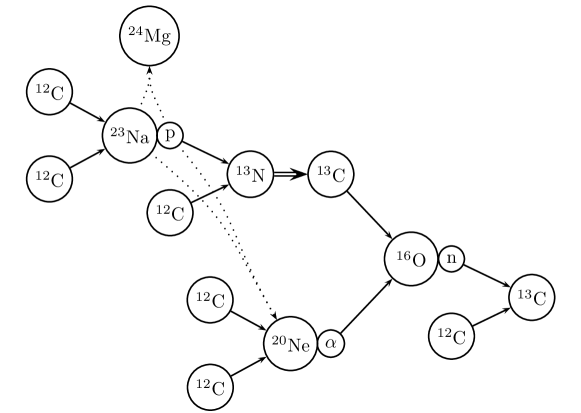
Figure 8: Same as Figure 3, but with proton leaks (dotted arrows). See discussion in the text for neutron and $\alpha$–leaks.

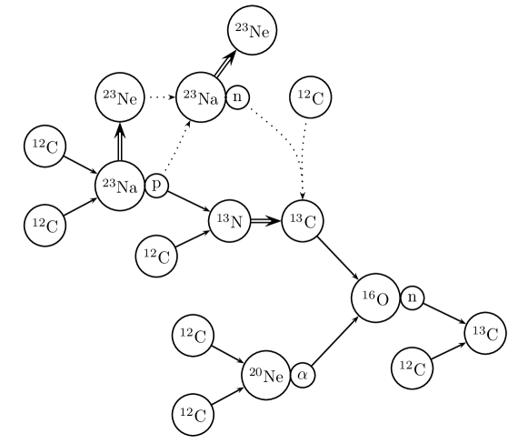
Figure 9: Same as Figure 4, but with proton leaks and the resulting bypass for neutron captures (dotted arrows). See discussion in the text for neutron and $\alpha$–leaks.

4.2 Neutron Leaks

A similar analysis can be done to compute the critical mole fraction of secondary nuclei for neutron leaks to be important. In this case, the most important neutron capture reactions are ${}^{12}{\rm C}(n,\gamma)^{13}{\rm C}$, ${}^{20}{\rm Ne}(n,\gamma)^{21}{\rm Ne}$, ${}^{21}{\rm Ne}(n,\gamma)^{22}{\rm Ne}$ and ${}^{23}{\rm Na}(n,\gamma)^{24}{\rm Na}$. The ${}^{20}{\rm Ne}$ and ${}^{21}{\rm Ne}$ neutron capture reactions have very similar cross–sections, approximately seven times the ${}^{12}{\rm C}$ neutron capture reaction. The ${}^{23}{\rm Na}$ reaction has a cross–section approximately 11 times bigger than the cross–section of the ${}^{12}{\rm C}$ neutron capture reaction.

The ratio of the mole fractions of ${}^{20}{\rm Ne}$ and ${}^{23}{\rm Na}$ with respect to ${}^{12}{\rm C}$ can be related to the mole fraction change of ${}^{12}{\rm C}$ using equations (31) and (32), at densities when the ${}^{23}{\rm Ne}$ $\beta$–decay time–scale is shorter than the ${}^{23}{\rm Na}$ $e^{-}$–capture time–scale:

$$Y(^{20}{\rm Ne})+Y(^{23}{\rm Na}) \approx-\Delta Y(^{12}{\rm C})~{}\biggl{\{}\frac{dY(^{20}{\rm Ne})}{dY(^{12}{\rm C})}+\frac{dY(^{23}{\rm Na})}{dY(^{12}{\rm C})}\biggr{\}}$$

$$\approx-0.34~{}\Delta Y(^{12}{\rm C}),$$ (40)

or when the ${}^{23}{\rm Na}$ $e^{-}$–capture is shorter than the ${}^{23}{\rm Ne}$ $\beta$–decay time–scale:

$$Y(^{20}{\rm Ne})+Y(^{23}{\rm Na})\approx-0.19~{}\Delta Y(^{12}{\rm C}).$$ (41)

In the first case, using equation (4.2) and using the added cross–sections of ${}^{20}{\rm Ne}$, ${}^{21}{\rm Ne}$ and ${}^{23}{\rm Na}$ neutron captures, it can be shown that neutron leaks, i.e. significant neutron captures on species different than ${}^{12}{\rm C}$, occur when the fraction of burnt carbon is approximately 12% its original amount. In the second case, using equation (41) it can be shown that neutron leaks will occur when about 38% of the original carbon is burnt.

As first noticed by Chamulak et al. (2007), neutron captures onto ${}^{56}{\rm Fe}$ will be negligible, since the ${}^{56}{\rm Fe}(n,\gamma)^{57}{\rm Fe}$ reaction has a cross–section approximately 64 times bigger than that of neutron capture onto ${}^{12}{\rm C}$, but the mole fraction of ${}^{56}{\rm Fe}$ is approximately 1250 times smaller than that of ${}^{12}{\rm C}$ at solar metallicity in the ${}^{12}{\rm C}$–rich environment of a WD. Thus, a ${}^{56}{\rm Fe}$ abundance of more than 20 times the solar abundance would be required to compete with the reaction ${}^{12}{\rm C}(n,\gamma)^{13}{\rm C}$.

4.3 $\alpha$–particle Leaks

Our detailed nuclear network shows that the most important reactions for $\alpha$–captures are ${}^{13}{\rm C}(\alpha,n)^{16}{\rm O}$, followed by the much weaker reactions ${}^{12}{\rm C}(\alpha,\gamma)^{16}{\rm O}$ and ${}^{16}{\rm O}(\alpha,\gamma)^{20}{\rm Ne}$. In Figure 10 we show the ratios of the mole fractions of ${}^{12}{\rm C}$ and ${}^{16}{\rm O}$ relative to the mole fraction of ${}^{13}{\rm C}$ necessary for ${}^{13}{\rm C}(\alpha,n)^{16}{\rm O}$ to be the dominant $\alpha$–capture reaction. It can be seen that only a minimal amount of ${}^{13}{\rm C}$ is needed for this to be the case: $Y(^{13}{\rm C})\approx 3\times 10^{-8}$, which is $\approx 10^{4}$ times lower than the solar metallicity value.

Moreover, using arguments similar to those used for proton and neutron leaks, a fraction of only $4\times 10^{-6}$ of the original ${}^{12}{\rm C}$ needs to be burnt to reproduce this abundance with zero metallicity, assuming that for every six ${}^{12}{\rm C}$ nuclei one ${}^{13}{\rm C}$ nucleus is produced. Thus, under the temperature range investigated here, one would conclude that these secondary reactions are negligible.

However, if significant neutron leaks occur, ${}^{13}{\rm C}$ can be significantly depleted and these reactions can become important. In fact, after ${}^{13}{\rm C}$ is depleted as a consequence of neutron leaks and the $\alpha$–particle over–production accompanying the ${}^{23}{\rm Na}(p,\alpha)^{20}{\rm Ne}$ proton leak reaction, $\alpha$–leaks are necessary to reproduce the abundances of ${}^{16}{\rm O}$, ${}^{20}{\rm Ne}$ and to limit the growth of $\alpha$–particles and reproduce the ${}^{13}{\rm C}$ depletion more accurately.

Figure 10: Number ratio of ${}^{12}{\rm C}$ or ${}^{16}{\rm O}$ to ${}^{13}{\rm C}$ when the rates of the $\alpha$–capture reactions ${}^{12}{\rm C}(\alpha,\gamma)^{16}{\rm O}$ or ${}^{16}{\rm O}(\alpha,\gamma)^{20}{\rm Ne}$ equals the rate of $\alpha$–captures in the reaction ${}^{13}{\rm C}(\alpha,n)^{16}{\rm O}$.

5 THE SIMPLIFIED NETWORK: SECOND APPROXIMATION (N2)

We can now include the leak reactions discussed in the previous section and additional ones with the following indices:

9)	${}^{23}{\rm Na}(p,\alpha)^{20}{\rm Ne}$,	Q = 2.38 MeV,	10)	${}^{23}{\rm Na}(p,\gamma)^{24}{\rm Mg}$,	Q = 11.69 MeV,
11)	${}^{23}{\rm Ne}(p,n)^{23}{\rm Na}$,	Q = 3.59 MeV,	12)	${}^{20}{\rm Ne}(n,\gamma)^{21}{\rm Ne}$,	Q = 6.76 MeV,
13)	${}^{23}{\rm Na}(n,\gamma)^{24}{\rm Na}$,	Q = 6.96 MeV,	14)	${}^{12}{\rm C}(\alpha,\gamma)^{16}{\rm O}$,	Q = 7.16 MeV,
15)	${}^{16}{\rm O}(\alpha,\gamma)^{20}{\rm Ne}$,	Q = 2.84 MeV,	16)	${}^{21}{\rm Ne}(n,\gamma)^{22}{\rm Ne}$,	Q = 10.36 MeV,
17)	${}^{13}{\rm C}(p,\gamma)^{14}{\rm N}$,	Q = 7.55 MeV,	18)	${}^{21}{\rm Ne}(p,\gamma)^{22}{\rm Na}$,	Q = 6.74 MeV,
19)	${}^{20}{\rm Ne}(\alpha,\gamma)^{24}{\rm Mg}$,	Q = 9.32 MeV,	20)	${}^{23}{\rm Ne}(\alpha,n)^{26}{\rm Mg}$,	Q = 5.41 MeV,
21)	${}^{23}{\rm Na}(\alpha,p)^{26}{\rm Mg}$,	Q = 1.82 MeV,	22)	${}^{21}{\rm Ne}(\alpha,n)^{26}{\rm Mg}$,	Q = 4.84 MeV,

This list includes proton–leak reactions (9, 10, 11, 17 and 18), neutron–leak reactions (12, 13 and 16), and $\alpha$–leak reactions (14, 15, 19, 20, 21 and 22). Proton–leaks are the first to be significant as ${}^{12}{\rm C}$ ashes are produced, but with more ashes produced neutron–leaks become relevant too. When this happens, ${}^{13}{\rm C}$ is rapidly depleted and $\alpha$–leaks become important as well.

As can be seen from the reactions in the list, it would be necessary to increase the number of species to account for all proton, neutron and $\alpha$–leaks exactly. To do this we can either account for ${}^{24}{\rm Mg}$, ${}^{21}{\rm Ne}$, ${}^{24}{\rm Na}$, ${}^{22}{\rm Ne}$, ${}^{14}{\rm N}$, ${}^{22}{\rm Na}$ and ${}^{26}{\rm Mg}$ independently, or we can group some or all of them into an auxiliary variable. Since reactions 16) and 18) depend on the abundance of ${}^{21}{\rm Ne}$ nuclei, we solve for ${}^{21}{\rm Ne}$ independently and group ${}^{24}{\rm Mg}$, ${}^{24}{\rm Na}$, ${}^{22}{\rm Ne}$, ${}^{14}{\rm N}$, ${}^{22}{\rm Na}$ and ${}^{26}{\rm Mg}$ into a dummy leak species.

Thus, while keeping the number of independent variables small and ensuring mass conservation, we can introduce $Y_{\rm L}$ as the mole fraction of a dummy nuclei that represents leaks on ${}^{24}{\rm Mg}$, ${}^{24}{\rm Na}$, ${}^{22}{\rm Ne}$, ${}^{14}{\rm N}$, ${}^{22}{\rm Na}$ and ${}^{26}{\rm Mg}$. We assume that this dummy species has approximately the average mass number of the species it represents, defining it as:

$$Y_{\rm L}\equiv\max\biggl{\{}0,~{}\frac{1-\sum A_{\rm i}Y_{\rm i}}{22}\biggr{\}}$$ (42)

where $A_{\rm i}$ is the mass number of the respective species and the sum is made over ${}^{12}{\rm C}$, ${}^{13}{\rm C}$, ${}^{13}{\rm N}$, ${}^{16}{\rm O}$, ${}^{20}{\rm Ne}$, ${}^{21}{\rm Ne}$, ${}^{23}{\rm Ne}$ and ${}^{23}{\rm Na}$. Since the leak nuclei ${}^{24}{\rm Mg}$, ${}^{24}{\rm Na}$, ${}^{22}{\rm Ne}$, ${}^{14}{\rm N}$ and ${}^{22}{\rm Na}$ can subsequently capture neutrons with a cross–sections similar to that of ${}^{20}{\rm Ne}$, for simplicity we will assume that leak nuclei capture neutrons with the ${}^{20}{\rm Ne}$ cross–section.

If we now add new terms associated to the $p$, $n$ and $\alpha$–leak reactions discussed above into equations (3) to (12) and assume a stationary solution for the trace nuclei $p,~{}\alpha,~{}n~{}\rm{and}~{}^{13}{\rm N}$, the modified equilibrium mole fractions can be described with the following equations (c.f. equations. 13):

$$\tilde{Y}(p) =\bar{Y}(p)~{}f_{\rm p}, \tilde{Y}(\alpha) =\bar{Y}(\alpha)~{}f_{\alpha},$$

$$\tilde{Y}(n) =\bar{Y}(n)~{}f_{\alpha}~{}f_{\rm n}, \tilde{Y}({{}^{13}{\rm N}}) =\bar{Y}({{}^{13}{\rm N}})~{}f_{\rm p},$$ (43)

where the auxiliary variable $f_{\rm p}$, $f_{\rm n}$ and $f_{\alpha}$ are defined as follows:

$$f_{\rm p} \equiv\biggl{\{}1+f_{\rm inv}~{}\frac{Y({{}^{23}{\rm Na}})(\lambda_{9}+\lambda_{10})+Y({{}^{23}{\rm Ne}})\lambda_{11}+Y({{}^{13}{\rm C}})\lambda_{17}+Y({{}^{21}{\rm Ne}})\lambda_{18}}{Y({{}^{12}{\rm C}})\lambda_{3}}\biggr{\}}^{-1}$$ (44)

$$K \equiv 1+\frac{Y({{}^{12}{\rm C}})\lambda_{14}+Y({{}^{16}{\rm O}})\lambda_{15}+Y({{}^{20}{\rm Ne}})\lambda_{19}+Y({{}^{23}{\rm Ne}})\lambda_{20}+Y({{}^{23}{\rm Na}})\lambda_{21}+Y({{}^{21}{\rm Ne}})\lambda_{22}}{Y({{}^{13}{\rm C}})\lambda_{5}}$$ (45)

$$f_{\alpha} \equiv K^{-1}~{}\biggl{\{}1+2~{}\frac{Y({{}^{23}{\rm Na}})\tilde{Y}(p)}{Y^{2}({{}^{12}{\rm C}})}~{}\frac{\lambda_{9}}{\lambda_{2}}\biggr{\}}$$ (46)

$$f_{\rm n} \equiv\biggl{\{}1+\frac{Y({{}^{23}{\rm Ne}})\bigl{[}\tilde{Y}(p)\lambda_{11}+\tilde{Y}(\alpha)\lambda_{20}\bigr{]}+Y({{}^{21}{\rm Ne}})Y(\alpha)\lambda_{22}}{Y({{}^{13}{\rm C}})\tilde{Y}(\alpha)\lambda_{5}}\biggr{\}}$$

$$~{}~{}~{}~{}\biggl{\{}1+\frac{\bigl{[}Y({{}^{20}{\rm Ne}})+Y_{\rm L}\bigr{]}\lambda_{12}+Y({{}^{21}{\rm Ne}})\lambda_{16}+Y({{}^{23}{\rm Na}})\lambda_{13}}{Y({{}^{12}{\rm C}})\lambda_{6}}\biggr{\}}^{-1},$$ (47)

where we have neglected the contribution to $f_{\rm p}$ from the leak reaction ${}^{23}{\rm Na}(\alpha,p)^{26}{\rm Mg}$, which is generally small. An exact solution that takes into account the additional protons from this or similar reactions can be obtained by multipliying the trace abundances $\tilde{Y}(p)$ and $\tilde{Y}({{}^{13}{\rm N}})$ by the factor $\{1+A\bar{Y}(\alpha)\}~{}\{1-A\bar{Y}(\alpha)B\tilde{Y}(p)\}^{-1}$, where $A\equiv 2Y({{}^{23}{\rm Na}})\lambda_{21}~{}\{Y^{2}({{}^{12}{\rm C}})\lambda_{1}\}^{-1}$ and $B\equiv 2K^{-1}Y({{}^{23}{\rm Na}})\lambda_{9}~{}\{Y^{2}({{}^{12}{\rm C}})\lambda_{2}\}^{-1}$. The factors $f_{\alpha}$ and $f_{\rm n}$ should be computed by using these modified values.

These formulae can be used to approach the leak regime of the network and can be easily generalized to include more leak reactions involving protons, neutrons or $\alpha$–particles. They predict a decrease in the number of free protons and ${}^{13}{\rm N}$ nuclei at equilibrium and the fact that this decrease starts later when the ${}^{23}{\rm Ne}$ $\beta$–decay time–scale is shorter than the ${}^{23}{\rm Na}$ $e^{-}$–capture time–scale, at low densities. Also, they explain the contribution to $\alpha$–particles from the proton leak reaction ${}^{23}{\rm Ne}(p,\alpha)^{20}{\rm Ne}$, the $\alpha$–leaks from ${}^{12}{\rm C}$ and ${}^{16}{\rm O}$ captures, the contribution to neutrons from the proton leak reaction ${}^{23}{\rm Ne}(p,\alpha)^{20}{\rm Ne}$ and the neutron depletion due to ${}^{20}{\rm Ne}$, ${}^{21}{\rm Ne}$ and ${}^{23}{\rm Na}$ neutron captures under our approximation, as well as a simple estimate of the neutron captures on ${}^{24}{\rm Mg}$, ${}^{24}{\rm Na}$, ${}^{22}{\rm Ne}$, ${}^{14}{\rm N}$ and ${}^{22}{\rm Na}$.

Now, we can rewrite the differential equations describing the evolution of the slowly varying nuclei ${}^{12}{\rm C}$, ${}^{13}{\rm C}$, ${}^{16}{\rm O}$, ${}^{20}{\rm Ne}$, ${}^{23}{\rm Na}$ and ${}^{23}{\rm Ne}$, using the new trace nuclei equilibrium values and including the leak reactions discussed above, i.e.:

$$\frac{dY({{}^{12}{\rm C}})}{dt}=-Y({{}^{12}{\rm C}})\rho N_{\rm A}\biggl{\{}Y({{}^{12}{\rm C}})(\lambda_{1}+\lambda_{2})+\frac{\tilde{Y}(p)\lambda_{3}}{f_{\rm inv}}+\tilde{Y}(n)\lambda_{6}+\tilde{Y}(\alpha)\lambda_{14}\biggr{\}},$$ (48)

$$\frac{dY({{}^{13}{\rm C}})}{dt}=Y({{}^{13}{\rm N}})\lambda_{4}+\rho N_{\rm A}\biggl{\{}Y({{}^{12}{\rm C}})\tilde{Y}(n)\lambda_{6}-Y({{}^{13}{\rm C}})\bigl{[}\tilde{Y}(\alpha)\lambda_{5}+\tilde{Y}(p)\lambda_{17}\bigr{]}\biggr{\}},$$ (49)

$$\frac{dY({{}^{16}{\rm O}})}{dt}=\rho N_{\rm A}\tilde{Y}(\alpha)\biggl{\{}Y({{}^{13}{\rm C}})\lambda_{5}+Y({{}^{12}{\rm C}})\lambda_{14}-Y({{}^{16}{\rm O}})\lambda_{15}\biggr{\}},$$ (50)

$$\frac{dY({{}^{20}{\rm Ne}})}{dt}=\rho N_{\rm A}\biggl{\{}\frac{Y^{2}({{}^{12}{\rm C}})}{2}\lambda_{2}+Y({{}^{23}{\rm Na}})\tilde{Y}(p)\lambda_{9}-Y({{}^{20}{\rm Ne}})\bigl{[}\tilde{Y}(n)\lambda_{12}+\tilde{Y}(\alpha)\lambda_{19}\bigr{]}$$

$$~{}~{}~{}~{}~{}~{}~{}~{}~{}~{}~{}~{}~{}+Y({{}^{16}{\rm O}})\tilde{Y}(\alpha)\lambda_{15}\biggr{\}},$$ (51)

$$\frac{dY({{}^{23}{\rm Na}})}{dt}=-Y({{}^{23}{\rm Na}})\lambda_{7}+Y({{}^{23}{\rm Ne}})\lambda_{8}+\rho N_{\rm A}\biggl{\{}\frac{Y^{2}({{}^{12}{\rm C}})}{2}\lambda_{1}+Y({{}^{23}{\rm Ne}})\tilde{Y}(p)\lambda_{11}$$

$$~{}~{}~{}~{}~{}-Y({{}^{23}{\rm Na}})\bigl{[}\tilde{Y}(p)(\lambda_{9}+\lambda_{10})+\tilde{Y}(n)\lambda_{13}+\tilde{Y}(\alpha)\lambda_{21}\bigr{]}\biggr{\}},$$ (52)

$$\frac{dY({{}^{23}{\rm Ne}})}{dt}=Y({{}^{23}{\rm Na}})\lambda_{7}-Y({{}^{23}{\rm Ne}})\lambda_{8}-Y({{}^{23}{\rm Ne}})\rho N_{\rm A}\bigl{[}\tilde{Y}(p)\lambda_{11}+\tilde{Y}(\alpha)\lambda_{20}\bigr{]},$$ (53)

$$\frac{dY({{}^{21}{\rm Ne}})}{dt}=\rho N_{\rm A}\biggl{\{}Y({{}^{20}{\rm Ne}})\tilde{Y}(n)\lambda_{12}-Y({{}^{21}{\rm Ne}})\bigl{[}\tilde{Y}(p)\lambda_{18}+\tilde{Y}(n)\lambda_{16}+\tilde{Y}(\alpha)\lambda_{22}\bigr{]}\biggr{\}}.$$ (54)

The energy generation rate can be obtained after a straightforward modification of the individual terms above, noting that the combined energy contribution of the inverse reaction ${}^{13}{\rm N}(\gamma,p)^{12}{\rm C}$ and the reaction ${}^{12}{\rm C}(p,\gamma)^{13}{\rm N}$ can be obtained simply by multiplying the Q–value of reaction 3) to the associated term in the r.h.s. of equation (48).

6 COMPARISON WITH THE DETAILED NETWORK

In what follows we will compare the results of the full nuclear network introduced in Section 2 with those of the simplified nuclear networks N1 and N2 introduced in Sections 3 and 5. We will compare the evolution of the main and trace nuclei mole fractions, the time evolution and the energy release in the form of photons or neutrinos as a function of the fraction of burnt ${}^{12}{\rm C}$ nuclei.

In most examples we have chosen a temperature of $4\times 10^{8}$ K and a density of $3\times 10^{9}$ g cm^-3, which are typical of the conditions encountered during the thermonuclear runaway and before ignition in a pre–supernova CO WD. We chose a temperature and density at which the simplified solution errors would be representative of those encountered at other temperatures and densities after the trace nuclei have reached their equilibrium values. The time–scales for the trace nuclei to reach their equilibrium values can be computed from equations (14).

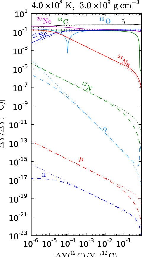
Figure 11: The ratio between the ashes and ${}^{12}{\rm C}$ mole fraction changes vs the fraction of burnt ${}^{12}{\rm C}$ in the full and N1 networks. Main ashes and the neutron excess change are shown as continuous (full network) or dot–dashed (N1) lines and trace nuclei are shown as dashed (full network) or dotted (N1) lines. See discussion in the text.

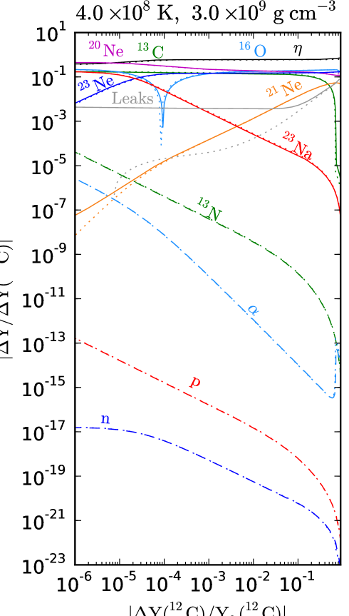
Figure 12: Same as Figure 11, but using the network N2 as comparison. We also include the mole fraction changes of ${}^{21}{\rm Ne}$ and the dummy leak particles introduced in equation (42). Note that the trace nuclei follow their equilibrium values precisely under this approximation. The abundance of leak nuclei is only well matched when more than $\approx$ 1% of the ${}^{12}{\rm C}$ is burnt.

In Figures 11 and 12 we show the ratio between the ${}^{12}{\rm C}$ ashes and ${}^{12}{\rm C}$ mole fraction changes vs the fraction of burnt ${}^{12}{\rm C}$, as well as the ratio between the neutron excess change and the ${}^{12}{\rm C}$ mole fraction change vs the fraction of burnt ${}^{12}{\rm C}$. We compare the integration of the full network with that of the networks N1 and N2, respectively. The transformation was chosen because it makes the evolution of ${}^{13}{\rm C}$, ${}^{16}{\rm O}$ and ${}^{20}{\rm Ne}$ look exactly flat under N1, according to equations (29), (30) and (31), allowing an easier comparison between the integrations of N1 and N2.

It can be seen that once the slowest evolving trace nuclei reach their equilibrium value and before about 1% of the ${}^{12}{\rm C}$ has been burnt, both plots show a good agreement between the simplified and full networks for the main ${}^{12}{\rm C}$ ashes. The exceptions are $\alpha$–particles, ${}^{16}{\rm O}$ and ${}^{20}{\rm Ne}$ under N1 due to the initial $\alpha$–leaks from reaction 15) and because we have assumed a pure CO mixture, with ${}^{13}{\rm C}$ initially absent. Since in this example the ${}^{23}{\rm Na}$ $e^{-}$–capture time–scale is shorter than the ${}^{23}{\rm Ne}$ $\beta$–decay time–scale, both simplified solutions correctly predict a higher abundance for ${}^{23}{\rm Ne}$ once both time–scales become comparable. Both solutions show a good match for the neutron excess changes too.

However, once the fraction of burnt ${}^{12}{\rm C}$ is above $\sim 1$%, the trace nuclei equilibrium abundances of N1 begin to differ from the exact solution, whereas N2 matches their values even when more than half of the original ${}^{12}{\rm C}$ has been burnt. The inclusion of the leak reactions in N2 provides a better match for the trace nuclei and as a consequence, the main ${}^{12}{\rm C}$ ashes as well, once the trace nuclei equilibrium mole fractions have been reached. Note also that the $\alpha$–particle, ${}^{16}{\rm O}$ and ${}^{20}{\rm Ne}$ mole fraction changes are well matched in N2 once trace nuclei equilibrium is reached.

In N2 the trace nuclei follow precisely their equilibrium values as ${}^{12}{\rm C}$ burns, even if these equilibrium values change dramatically. This is because their characteristic time–scales are much smaller than the characteristic ${}^{12}{\rm C}$ burning time–scale. This supports the use of N2 in a varying temperature and density integration, which would be analogous to changing the equilibrium values of the trace nuclei as ${}^{12}{\rm C}$ burns. The shortest time–scale for the environment’s variables to change should be bigger than the biggest trace nuclei time–scale.

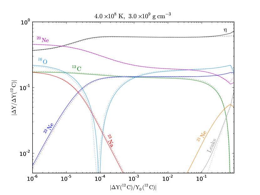
Figure 13: The ratio between the main ashes and ${}^{12}{\rm C}$ mole fraction changes vs the fraction of burnt ${}^{12}{\rm C}$ in the full (continuous) and N2 (dot–dashed) networks. Note that in N1 the evolution of the species ${}^{13}{\rm C}$, ${}^{16}{\rm O}$ and ${}^{20}{\rm Ne}$ should be exactly flat in this plot according to equations (29), (30) and (31). Generally speaking, N2 reproduces the full network abundances to the 5% level when the trace nuclei have reached their equilibrium mole fractions. In numerical experiments, N2 loses its accuracy when both $f_{\rm p}$ and $f_{\alpha}$ (see equations 44 and 5) are lower than 0.5, which is due to the observed ${}^{13}{\rm C}$ depletion.

In Figure 13 we show an enlarged section of Figure 12. If N1 were valid, the evolution of ${}^{16}{\rm O}$ and ${}^{20}{\rm Ne}$ would look flat and approximately 0.19 in this space. The same would be the case for ${}^{13}{\rm C}$, although approximately 0.15 (see equations 29, 30 and 31). This is only approximately true when the fraction of burnt ${}^{12}{\rm C}$ is between 2% and 5%. Since we plot absolute values of mole fraction changes, Figure 13 does not show whether the ${}^{16}{\rm O}$ mole fraction is decreased or increased. In fact, its mole fraction is originally depleted and, only after the fraction of burnt ${}^{12}{\rm C}$ is about $10^{-4}$, it is increased. The original depletion is caused by $\alpha$–leaks in reaction 15), which increase the mole fraction of ${}^{20}{\rm Ne}$.

The ${}^{23}{\rm Ne}$ mole fraction is larger than the ${}^{23}{\rm Ne}$ mole fraction only after the burnt fraction of ${}^{12}{\rm C}$ is about $2\times 10^{-5}$. Interestingly, this makes the neutron excess evolution change from above $0.3$ to $0.6$ in this transformation. This can be understood noticing that $d\eta/dt=-2dY_{\rm e}/dt$ and that the value shown in equation (34) is expected to double at high density.

Note that ${}^{13}{\rm C}$ is depleted as ${}^{21}{\rm Ne}$ and leak nuclei increase their abundance. This is because neutron leaks shortcut ${}^{13}{\rm C}$ neutron captures, as discussed before. When this happens, $f_{\alpha}$ decreases dramatically (see equation 46), and the accuracy of the approximation is lost to about 20% level. Although at the beginning of the integration $f_{\alpha}$ is also small, N2 matches the full network with great accuracy. To distinguish between the cases when the accuracy of N2 is very good and only a small fraction of ${}^{12}{\rm C}$ has been burnt from the late loss of accuracy with a big fraction of ${}^{12}{\rm C}$ burnt, we define the criterion for N2 to be considered an accurate representation of the full network as

$$f_{\rm p}>0.5~{}~{}~{}~{}{\rm and}~{}~{}~{}~{}~{}f_{\alpha}>0.5,$$ (55)

which should be used in a varying temperature and density integration, such as in real stellar evolution models.

In Figure 14 we show a similar integration as in Figure 13, but at a density of $10^{9}$ g cm^-3. We can see that ${}^{13}{\rm C}$ is depleted at a smaller fraction of ${}^{12}{\rm C}$ than in Figure 13. This is because there are more leak nuclei to capture neutrons. The same associated loss of accuracy after ${}^{13}{\rm C}$ depletion is observed. We can also see that the neutron excess evolution is closer to 0.3 in this Figure, as expected from equation (34). However, as ${}^{13}{\rm C}$ is depleted, the e^-–capture rate decreases accordingly and the neutron excess evolution becomes slower.

Finally, note that although by introducing the dummy leak nuclei we can keep the number of independent variables small, we will necessarily lose some accuracy matching the neutron excess. Many leak nuclei can capture protons, neutrons or $\alpha$–particles, but they can also capture electrons like ${}^{23}{\rm Na}$ does. Electron captures on free protons were found to be negligible. In order of increasing density, or Fermi electron energy, the following reactions may compete with proton, neutron and $\alpha$–captures:  ${}^{22}{\rm Na}(e^{-},\nu_{e})^{22}{\rm Ne}$, ${}^{24}{\rm Na}(e^{-},\nu_{e})^{24}{\rm Ne}$, ${}^{25}{\rm Mg}(e^{-},\nu_{e})^{25}{\rm Ne}$, ${}^{24}{\rm Mg}(e^{-},\nu_{e})^{24}{\rm Na}$ or ${}^{21}{\rm Ne}(e^{-},\nu_{e})^{21}{\rm F}$, affecting the neutron excess evolution (see Iben, 1978).

It is not possible to model the former electron captures accurately without solving for each leak species and its electron capture counterpart independently. Moreover, the relative abundances of the different leak species will depend on the temperature and density history of the gas, which makes it very difficult to compute the contribution of the different electron capture reactions knowing only $Y_{\rm L}$. However, assuming that the excess of neutrons over protons of the leak nuclei is 1.5 under N2, a 10% or 20% accuracy for the neutron excess evolution was achieved before and after ${}^{13}{\rm C}$ depletion, respectively. This translates into a maximum of 5% or 10% error for the electron fraction, normally below 1% for small quantities of burnt ${}^{12}{\rm C}$.

Figure 14: Same as Figure 14, but changing the density to $10^{9}$ g cm^-3. We can see that the network N2 loses its accuracy at a lower fraction of burnt ${}^{12}{\rm C}$, which is due to stronger neutron leaks which cause ${}^{13}{\rm C}$ to be relatively depleted sooner.

6.0.1 Timing and Energy Generation Comparison

In Figure 15 we show the ratio between the elapsed times of the simplified and full integrations vs the fraction of burnt ${}^{12}{\rm C}$. The N1 and N2 sub–scripts correspond to the solution of the first and second simplified networks, respectively. We can see that the N1 can over–estimate the speed at which ${}^{12}{\rm C}$ burns by more than 20%, whereas the second simplified network reproduces the time evolution to better than 5% error. This is due to the absence of leak reactions in the first approximation, which over–estimates the amount of ${}^{12}{\rm C}$ proton and neutron captures at a given time.

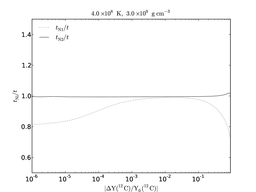
Figure 15: The ratio between the elapsed time in the two simplified networks and the full nuclear network plotted against the fraction of burnt ${}^{12}{\rm C}$. N1 and N2 sub–scripts indicate which simplified network has been used for the comparison.

In Figure 16 we show the ratios between the photon and neutrino energy release rates in N1 and N2 and the photon and neutrino energy release rate in the full network. We can see that the photon energy release rates is typically off in N1 by 20% or more, whereas N2 matches them at the 5% level, except after ${}^{13}{\rm C}$ is depleted. This is because the leak reactions tend to release more energy than the ${}^{12}{\rm C}$ proton and neutron captures. The neutrino energy release rates are not as accurate because secondary electron captures not included in these networks can have an important contribution, but since photon energy rates are generally much bigger, the error in the net energy release remains at the 5% level.

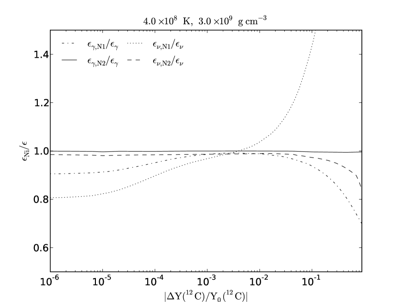
Figure 16: Same as Figure 15, but we now show the ratios of the photon and neutrino energy release rates between the simplified and the full networks. N1 and N2 sub–scripts indicate which simplified network has been used for the comparison.

7 DISCUSSION AND CONCLUSIONS

We have derived two approximate nuclear networks that can be used in the hydrostatic carbon burning regime of carbon–oxygen white dwarfs (CO WDs) approaching ignition. The networks have the advantage of being able to track accurately the relevant species during this phase of evolution without having to include the fast–evolving protons, neutrons, $\alpha$–particles or ${}^{13}{\rm N}$ nuclei.

Using the same integration method (Bader & Deuflhard, 1983), convergence tolerance and initial conditions in one–zone models, we have found that the integration of N1 or N2 is much faster than that of the detailed network. Depending on the temperature, density and composition, the ratio between the integration times of the detailed network and N2 varied between a factor of a few and a factor of several hundreds. Integration time ratios between N2 and N1 varied between 1.2 and 1.3. Note that the slowest step in the integration of full stellar evolution models is normally Gaussian elimination or similar methods, which scale with the cube of the number of independent physical variables. Thus, the simplified networks presented in this work could have important applications in full stellar evolution models.

Depending on the amount of ${}^{12}{\rm C}$ being burnt and the desired errors in the mole fractions of the dominant nuclei, the time and the net energy release, either the N1 or N2 approximations described in Sections 3 and 5 could be used in CO WD interiors. For an accuracy of the order of 50%, and to have a simple picture of the main flows involved, N1 can be used with caution. For an accuracy of the order of 5%, N2 should be used instead. If N2 is used and the criterion in equation (55) does not hold, only an accuracy of the order of 20% can be guaranteed, as long as all the trace nuclei time–scales are much shorter than the ${}^{12}{\rm C}$–burning time–scale.

These accuracies are not valid for nuclei whose mole fractions are not significant, for example ${}^{23}{\rm Ne}$ when the $\beta$–decay time–scale is much shorter than the $e^{-}$–capture time–scale, since in this case the ${}^{22}{\rm Ne}(n,\gamma)^{23}{\rm Ne}$ reaction will dominate its evolution, a reaction that cannot be included accurately under N2. We have also found that for relatively low densities, below $10^{8}$ g cm^-3, the quoted errors can double, but only when significant amounts of ${}^{12}{\rm C}$ have been burnt, which normally occurs when the density is significantly above this number. Thus, N2 is more accurate for central ignition models, but it could also be used in off–center ignition models.

We have shown how to derive the approximations and have compared them to a detailed network at fixed temperature and density. We have also discussed how the approximations can break down and when they can be used. Since all the details of the derivation are shown, these simplified networks can be further improved straightforwardly. It is also possible to build intermediate approximations between N1 and N2, for example, including ${}^{21}{\rm Ne}$ in the dummy leak species defined in equation (42) to remove one independent variable from the solution. We have tested this last approximation in a few cases and the resulting errors appears to be twice the errors in N2.

Although for simplicity we have only shown fixed temperature and density integrations, these approximations can be used in environments with varying temperature and density, such as real stellar evolution models. This is because in the temperature and density range found in pre–ignition WD interiors the trace nuclei reach their equilibrium values much faster than the typical environmental variables vary inside the star, even within strong pre–ignition convective velocity fields.

The networks can account for ${}^{23}{\rm Na}$ or ${}^{13}{\rm N}$ $e^{-}$–captures for the purposes of following the evolution of the pressure–supporting electrons in pre–supernova WDs. We have shown that they will be valid even in convective WD interiors. We recommend the use of these networks when the mass fractions of the most abundant species are relevant, namely ${}^{12}{\rm C}$, ${}^{16}{\rm O}$, ${}^{13}{\rm C}$, ${}^{20}{\rm Ne}$, ${}^{23}{\rm Ne}$ or ${}^{23}{\rm Na}$, or the electron mole fraction, $Y_{\rm e}$, or the energy generation rates. We do not recommend its use if the abundances of other nuclei not included in this discussion are being studied.

We have introduced an important tool to understand the effect of the convective Urca process on the ignition conditions of SNe Ia. We foresee the application of these simplified networks or their modification in detailed one or multi–dimensional stellar evolution models trying to understand pre–supernova CO WDs or similar objects (see e.g. Lesaffre et al., 2006; Zingale et al., 2009; Iapichino & Lesaffre, 2010).

References

- Bader & Deuflhard (1983) Bader, G., Deuflhard, P. 1983, Numer. Math. 41, 373-398
- Barkat & Wheeler (1990) Barkat, Z., & Wheeler, J. C. 1990, ApJ, 355, 602
- Bruenn (1973) Bruenn, S. W. 1973, ApJ, 183, L125
- Chamulak et al. (2007) Chamulak, D. A., Brown, E. F., & Timmes, F. X. 2007, ApJ, 655, L93
- Chamulak, Brown, Timmes, & Dupczak (2008) Chamulak, D. A., Brown, E. F., Timmes, F. X., & Dupczak, K. 2008, ApJ, 677, 160
- Couch & Arnett (1974) Couch, R. G., & Arnett, D. W. 1974, ApJ, 194, 537
- Domínguez et al. (2006) Domínguez, I., Piersanti, L., Bravo, E., Tornambé, A., Straniero, O., & Gagliardi, S. 2006, ApJ, 644, 21
- Gasques et al. (2005) Gasques, L. R., Afanasjev, A. V., Aguilera, E. F., Beard, M., Chamon, L. C., Ring, P., Wiescher, M., & Yakovlev, D. G. 2005, Phys. Rev. C, 72, 025806
- Graboske, Dewitt, Grossman, & Cooper (1973) Graboske, H. C., Dewitt, H. E., Grossman, A. S., & Cooper, M. S. 1973, ApJ, 181, 457
- Hachisu, Kato, & Nomoto (1996) Hachisu, I., Kato, M., & Nomoto, K. 1996, ApJ, 470, L97
- Hachisu, Kato, & Nomoto (1999) Hachisu, I., Kato, M., & Nomoto, K. 1999, ApJ, 522, 487
- Hachisu, Kato, Nomoto, & Umeda (1999) Hachisu, I., Kato, M., Nomoto, K., & Umeda, H. 1999, ApJ, 519, 314
- Hamuy et al. (1996) Hamuy, M., Phillips, M. M., Suntzeff, N. B., Schommer, R. A., Maza, J., & Aviles, R. 1996, AJ, 112, 2391
- Han & Podsiadlowski (2004) Han, Z., & Podsiadlowski, Ph. 2004, MNRAS, 350, 1301
- Hillebrandt & Niemeyer (2000) Hillebrandt, W., & Niemeyer, J. C. 2000, ARA&A, 38, 191
- Kasen, Röpke, & Woosley (2009) Kasen, D., Röpke, F. K., & Woosley, S. E. 2009, Nature, 460, 869
- Khokhlov (1991) Khokhlov, A. M. 1991, A&A, 245, 114
- Kromer & Sim (2009) Kromer, M., & Sim, S. A. 2009, MNRAS, 398, 1809
- Iapichino, Brüggen, Hillebrandt, & Niemeyer (2006) Iapichino, L., Brüggen, M., Hillebrandt, W., & Niemeyer, J. C. 2006, A&A, 450, 655
- Iapichino & Lesaffre (2010) Iapichino, L., & Lesaffre, P. 2010, arXiv:1001.2165. Accepted for publication in A&A.
- Iben (1978) Iben, I., Jr. 1978, ApJ, 219, 213
- Iben (1978) Iben, I., Jr. 1978, ApJ, 226, 996
- Iben (1982) Iben, I., Jr. 1982, ApJ, 253, 248
- Iben & Tutukov (1984) Iben, I., Jr., & Tutukov, A. V. 1984, ApJS, 54, 335
- Langer, Deutschmann, Wellstein, Hoeflich (2000) Langer, N., Deutschmann, A., Wellstein, S., Hoeflich, P. 2000, A&A, 362, 1046
- Lesaffre, Podsiadlowski, & Tout (2005) Lesaffre, P., Podsiadlowski, Ph., & Tout, C. A. 2005, MNRAS, 356, 131
- Lesaffre et al. (2006) Lesaffre, P., Han, Z., Tout, C. A., Podsiadlowski, Ph., & Martin, R. G. 2006, MNRAS, 368, 187
- Li & van den Heuvel (1997) Li, X.-D., & van den Heuvel, E. P. J. 1997, A&A, 322, L9
- Maeda et al. (2010) Maeda, K., et al. 2010, Nature, 466, 82
- Mazzali & Podsiadlowski (2006) Mazzali, P. A., & Podsiadlowski, Ph. 2006, MNRAS, 369, L19
- Mazzali, Röpke, Benetti, & Hillebrandt (2007) Mazzali, P. A., Röpke, F. K., Benetti, S., & Hillebrandt, W. 2007, Science, 315, 825
- Meng, Chen, & Han (2009) Meng, X., Chen, X., & Han, Z. 2009, MNRAS, 395, 2103
- Mochkovitch (1996) Mochkovitch, R. 1996, A&A, 311, 152
- Nomoto, Thielemann, & Yokoi (1984) Nomoto, K., Thielemann, F.-K., & Yokoi, K. 1984, ApJ, 286, 644
- Nomoto & Kondo (1991) Nomoto, K., & Kondo, Y. 1991, ApJ, 367, L19
- Nomoto, Saio, Kato, & Hachisu (2007) Nomoto, K., Saio, H., Kato, M., & Hachisu, I. 2007, ApJ, 663, 1269
- Oda et al. (1994) T. Oda, M. Hino, K. Muto, M. Takahara and K. Sato; Atomic Data and Nuclear Data Tables, 56, 231-403.
- Paczyński (1972) Paczyński, B. 1972, Astrophys. Lett., 11, 53
- Pakmor et al. (2010) Pakmor, R., Kromer, M., Röpke, F. K., Sim, S. A., Ruiter, A. J., & Hillebrandt, W. 2010, Nature, 463, 61
- Perlmutter et al. (1999) Perlmutter, S., et al. 1999, ApJ, 517, 565
- Phillips (1993) Phillips, M. M. 1993, ApJ, 413, L105
- Piro & Bildsten (2008) Piro, A. L., & Bildsten, L. 2008, ApJ, 673, 1009
- Pskovskii (1977) Pskovskii, I. P. 1977, Soviet Ast., 21, 675
- Regev & Shaviv (1975) Regev, O., & Shaviv, G. 1975, Ap&SS, 37, 143
- Riess et al. (1998) Riess, A. G., et al. 1998, AJ, 116, 1009
- Röpke et al. (2007) Röpke, F. K., Hillebrandt, W., Schmidt, W., Niemeyer, J. C., Blinnikov, S. I., & Mazzali, P. A. 2007, ApJ, 668, 1132
- Röpke & Niemeyer (2007) Röpke, F. K., & Niemeyer, J. C. 2007, A&A, 464, 683
- Röpke (2007) Röpke, F. K. 2007, ApJ, 668, 1103
- Spillane et al. (2007) Spillane, T., et al. 2007, Physical Review Letters, 98, 122501
- Stancliffe (2006) Stancliffe, R. J. 2006, MNRAS, 370, 1817
- Stein et al. (1999) Stein, J., Barkat, Z., & Wheeler, J. C. 1999, ApJ, 523, 381
- Sullivan et al. (2006) Sullivan, M., et al. 2006, ApJ, 648, 868
- Thielemann et al. (2006) Thielemann, F., et al. 1987, Adv. Nuc. Astro, 525.
- Webbink (1984) Webbink, R. F. 1984, ApJ, 277, 355
- Woosley, Kasen, Blinnikov, & Sorokina (2007) Woosley, S. E., Kasen, D., Blinnikov, S., & Sorokina, E. 2007, ApJ, 662, 487
- Yakovlev et al. (2006) Yakovlev, D. G., Gasques, L. R., Afanasjev, A. V., Beard, M., & Wiescher, M. 2006, Phys. Rev. C, 74, 035803
- Yoon, Podsiadlowski, & Rosswog (2007) Yoon, S.-C., Podsiadlowski, Ph., & Rosswog, S. 2007, MNRAS, 380, 933
- Zegers et al. (2008) Zegers, R. G. T., et al. 2008, Phys. Rev. C, 77, 024307
- Zingale et al. (2009) Zingale, M., Almgren, A. S., Bell, J. B., Nonaka, A., & Woosley, S. E. 2009, ApJ, 704, 196