APPLICATIONS OF VARIATIONAL ANALYSIS TO A GENERALIZED FERMAT-TORRICELLI PROBLEM
BORIS S. MORDUKHOVICH and NGUYEN MAU NAM

Abstract. In this paper we develop new applications of variational analysis and generalized differentiation to the following optimization problem and its specifications: given $n$ closed subsets of a Banach space, find such a point for which the sum of its distances to these sets is minimal. This problem can be viewed as an extension of the celebrated Fermat-Torricelli problem: given three points on the plane, find another point such that the sum of its distances to the designated points is minimal. The generalized Fermat-Torricelli problem formulated and studied in this paper is of undoubted mathematical interest and is promising for various applications including those frequently arising in location science, optimal networks, etc. Based on advanced tools and recent results of variational analysis and generalized differentiation, we derive necessary as well as necessary and sufficient optimality conditions for the extended version of the Fermat-Torricelli problem under consideration, which allow us to completely solve it in some important settings. Furthermore, we develop and justify a numerical algorithm of the subgradient type to find optimal solutions in convex settings and provide its numerical implementations.
Key words: Variational analysis and optimization, generalized Fermat-Torricelli problem, minimal time function, Minkowski gauge, generalized differentiation, necessary and sufficient optimality conditions, subgradient-type algorithms.
Mathematical Subject Classification (2000): 49J52, 49J53, 90C31.

1 Introduction and Problem Formulation

In the early 17th century Pierre de Fermat proposed the following problem: given three points on the plane, find a fourth point such that the sum of its Euclidean distances to the three given points is minimal. This problem was solved by Evangelista Torricelli and was named the Fermat-Torricelli problem. Torricelli’s solution states the following: if none of the interior angles of the triangle formed by the three fixed points reaches or exceeds $120^{\circ}$, the minimizing point in question is located inside this triangle in such a way that each side of the triangle is seen at an angle of $120^{\circ}$; otherwise it is the obtuse vertex of the triangle. This point is often called the Fermat-Torricelli point.

In the 19th century Jakob Steiner examined this problem in further depth and extended it to include a finitely many points on the plane. A number of other extensions have been proposed and studied over the years. This and related topics have nowadays attracted strong attention of many mathematicians and applied scientists; see, e.g., [3, 4, 11, 20] with the references therein for the history, various extensions, modifications, and applications to location science, statistics, optimal networks, etc. Note that, despite beautiful solutions obtained for particular extensions of the Fermat-Torricelli problem, we are not familiar with theoretical methods and/or numerical algorithms developed in rather general settings. We particularly refer the reader to [6, 10, 21] and the bibliographies therein to Weiszfeld’s algorithm and its modifications for the problem of minimizing weighted sums of Euclidean norms (also known as the Weber problem) and to [1] for efficient interior point type methods for similar problems in finite-dimensional spaces.

In this paper we study a far-going generalization of the Fermat-Torricelli problem that is formulated below. It extends, in particular, a generalized version of the classical Steiner (and Weber) versions with replacing given points therein by a finitely many closed sets in Banach spaces. Furthermore, our new extension of the Fermat-Torricelli problem covers a fast majority of the previous ones and seems to be interesting for both the theory and applications to various location models, optimal networks, wireless communications, etc.

We propose to employ powerful tools of modern variational analysis and generalized differentiation to study the extended version of Fermat-Torricelli problem and its specification from the theoretical/qualitative and numerical/algorithmic viewpoints. In the first direction our goal is to derive necessary as well as necessary and sufficient optimality conditions for generalized Fermat-Torricelli points and then to use them for explicit determining these points in some remarkable settings. Our numerical analysis involves developing an algorithm of the subgradient type and considering its specifications and implementations in the case of the generalized Fermat-Torricelli problem determined by an arbitrary number of convex sets in finite-dimensional spaces.

Let us now formulate the generalized Fermat-Torricelli problem of our study. Consider the so-called minimal time function

$$T^{F}_{\Omega}(x):=\inf\big{\{}t\geq 0\big{|}\;\Omega\cap(x+tF)\neq\emptyset\big{\}}$$ (1.1)

with the constant dynamics $\dot{x}\in F$ described by a closed, bounded, and convex subset $F\neq\emptyset$ of a Banach space $X$ and with the closed target set $\Omega\neq\emptyset$ in $X$; these are our standing assumptions in this paper. We refer the reader to [7, 8, 9, 15] and the bibliographies therein for various results on minimal time functions and their applications. When $F$ is the closed unit ball $I\!\!B$ of $X$, the minimal time function (1.1) becomes the standard distance function

$$\mbox{d}(x;\Omega)=\inf\big{\{}\|x-\omega\|\;\big{|}\;\omega\in\Omega\big{\}}$$ (1.2)

generated by the norm $\|\cdot\|$ on $X$. Given now an arbitrary number of closed subsets $\Omega_{i}\neq\emptyset$, $i=1,\ldots,n$, of $X$, we introduce the generalized Fermat-Torricelli problem as follows:

$$\mbox{minimize }\;T(x):=\sum_{i=1}^{n}T^{F}_{\Omega_{i}}(x),\quad x\in X.$$ (1.3)

For $F=I\!\!B$ in (1.3) this problem reduces to

$$\mbox{minimize }\;\mbox{D}(x):=\sum_{i=1}^{n}\mbox{d}(x;\Omega_{i}),$$ (1.4)

which corresponds to the Steiner-type extension of the Fermat-Torricelli problem in Banach spaces when all the sets $\Omega_{i}$, $i=1,\ldots,n$, are singletons. Observe that even in the latter classical case the optimization problem (1.3) and its specification (1.4) are nonsmooth while being convex if all the sets $\Omega_{i}$ have this property. It is thus natural to study these problems by means of advanced tools of variational analysis and generalized differentiation.

The rest of the paper is organized as follows. In Section 2 we define and discuss basic tools of variational analysis needed for formulations and proofs of the main results of this paper. Section 3 is devoted to computing and estimating subdifferentials of minimal time functions that play a crucial role in our study of the generalized Fermat-Torricelli problem and its specifications. In Section 4 we derive necessary conditions for the general problem (1.3) in Banach spaces as well as necessary and sufficient conditions in the case of convexity, which are then used for complete descriptions of Fermat-Torricelli points in some important settings. Finally, Section 5 presents and justifies a numerical algorithm for solving the generalized Fermat-Torricelli problem with convex data in finite-dimensional spaces.

Throughout the paper we use standard notation and terminology of variational analysis; see, e.g., [13, 18]. Recall that, given a set-valued mapping $G\colon X\;{\lower 1.0pt\hbox{$\rightarrow$}}\kern-10.0pt\hbox{\raise 2.0pt\hbox{$\rightarrow$}}\;X^{*}$ between a Banach space $X$ and its topological dual $X^{*}$, the sequential Painlevé-Kuratowski upper/outer limit as $x\to\bar{x}$ is defined by

$$\begin{array}[]{ll}\displaystyle\mathop{{\rm Lim}\,{\rm sup}}_{x\to\bar{x}}G(x):=\Big{\{}x^{*}\in X^{*}\Big{|}&\exists\,\mbox{ sequences }\;x_{k}\to\bar{x},\;x^{*}_{k}\stackrel{{\scriptstyle w^{*}}}{{\to}}x^{*}\;\mbox{ as }\;k\to\infty\\ &\mbox{such that }\;x^{*}_{k}\in G(x_{k})\;\mbox{ for all }\;k\in I\!\!N:=\{1,2,\ldots\}\Big{\}},\end{array}$$ (1.7)

where $w^{*}$ signifies the weak^∗ topology of $X^{*}$. For a set $\Omega\subset X$ the symbol $x\stackrel{{\scriptstyle\Omega}}{{\to}}\bar{x}$ means that $x\to\bar{x}$ with $x\in\Omega$. If $\varphi\colon X\to\overline{I\!\!R}:=(-\infty,\infty]$ is an extended-real-valued function finite at $\bar{x}$, the symbol $x\stackrel{{\scriptstyle\varphi}}{{\to}}\bar{x}$ signifies the convergence $x\to\bar{x}$ with $\varphi(x)\to\varphi(\bar{x})$.

2 Tools of Variational Analysis

In this section we briefly review some basic constructions and results of the generalized differentiation theory in variational analysis that are widely used in what follows. The reader can find all the proofs, discussions, and additional material in the books [6, 13, 14, 18, 19] and the references therein in both finite and infinite dimensions. Unless otherwise stated, all the spaces under consideration are Banach with the norm $\|\cdot\|$ and the canonical pairing $\langle\cdot,\cdot\rangle$ between the space in question and its topological dual.

Let us start with convex functions $\varphi\colon X\to\overline{I\!\!R}$. Given $\bar{x}\in\mbox{\rm dom}\,\varphi:=\{x\in X|\;\varphi(x)<\infty\}$, the subdifferential (collection of subgradients) of $\varphi$ at $\bar{x}$ in the sense of convex analysis is

$$\partial\varphi(\bar{x}):=\big{\{}x^{*}\in X^{*}\big{|}\;\langle x^{*},x-\bar{x}\rangle\leq\varphi(x)-\varphi(\bar{x})\;\mbox{ for all }\;x\in X\big{\}}.$$ (2.1)

Directly from definition (2.1) we have the following nonsmooth counterpart of the classical Fermat stationary rule for convex functions:

$$\bar{x}\;\mbox{ is a minimizer of }\;\varphi\;\mbox{ if and only if }\;0\in\partial\varphi(\bar{x}).$$ (2.2)

The subdifferential of convex analysis (2.1) satisfies a number of important calculus rules that are mainly based on separation theorems for convex sets. The central calculus result is the following Moreau-Rockafellar theorem for representing the subdifferential of sums.

Theorem 2.1

(subdifferential sum rule for convex functions). Let $\varphi_{i}\colon X\to\overline{I\!\!R}$, $i=1,\ldots,m$, be convex lower semicontinuous functions on a Banach space $X$. Assume that there is a point $\bar{x}\in\cap_{i=1}^{n}\mbox{\rm dom}\,\varphi_{i}$ at which all (except possibly one) of the functions $\varphi_{1},\ldots,\varphi_{m}$ are continuous. Then we have the equality

$$\partial\Big{(}\sum_{i=1}^{m}\varphi_{i}\Big{)}(\bar{x})=\sum_{i=1}^{m}\partial\varphi_{i}(\bar{x}).$$

Given a convex set $\Omega\subset X$ and a point $\bar{x}\in\Omega$, the corresponding geometric counterpart of (2.1) is the normal cone to $\Omega$ at $\bar{x}$ defined by

$$N(\bar{x};\Omega)=\big{\{}x^{*}\in X^{*}\big{|}\;\langle x^{*},x-\bar{x}\rangle\leq 0\;\mbox{ for all }\;x\in\Omega\big{\}},$$ (2.3)

which is in fact the subdifferential (2.1) of the set indicator function $\delta(x;\Omega)$ at $\bar{x}$ that is equal to $0$ for $x\in\Omega$ and to $\infty$ for $x\notin\Omega$.

Besides the aforementioned convex constructions suitable for the study of the generalized Fermat-Torricelli problem (1.3) in the case of convex sets $\Omega_{i}$, we need in what follows their extensions to nonconvex objects.

Given an arbitrary extended-real-valued function $\varphi\colon X\to\overline{I\!\!R}$ finite at $\bar{x}$ and given $\varepsilon\geq 0$, define first the $\varepsilon$-subdifferential of $\varphi$ at $\bar{x}$ by

$$\widehat{\partial}_{\varepsilon}\varphi(\bar{x}):=\Big{\{}x^{*}\in X^{*}\Big{|}\;\liminf_{x\to\bar{x}}\frac{\varphi(x)-\varphi(\bar{x})-\langle x^{*},x-\bar{x}\rangle}{\|x-\bar{x}\|}\geq-\varepsilon\Big{\}}.$$ (2.4)

For $\varepsilon=0$ the set $\widehat{\partial}\varphi(\bar{x}):=\widehat{\partial}_{0}\varphi(\bar{x})$ is known as regular/viscosity/Fréchet subdifferential of $\varphi$ at $\bar{x}$; it reduces to the classical gradient $\{\nabla\varphi(\bar{x})\}$ when $\varphi$ is Fréchet differentiable at this point and to the subdifferential (2.1) when $\varphi$ is convex. However, being naturally and rather simply defined, the Fréchet subdifferential and its $\varepsilon$-enlargements (2.4) do not possess—apart from locally convex settings and the like—a number of required calculus and related properties. For example, $\widehat{\partial}\varphi(\bar{x})$ may often be empty (e.g., for $\varphi(x)=-|x|$) and an analog of the sum rule from Theorem 2.1 does not hold for $\widehat{\partial}\varphi(\bar{x})$ whenever $\varepsilon\geq 0$; e.g., in the case of $\varphi_{1}(x)=|x|$ and $\varphi_{2}(x)=-|x|$.

The situation dramatically changes when we employ a sequential regularization of the $\varepsilon$-subdifferentials (2.4) defined by

$$\partial\varphi(\bar{x}):=\mathop{{\rm Lim}\,{\rm sup}}_{\scriptstyle{x\xrightarrow{\varphi}\bar{x}}\atop\scriptstyle{\varepsilon\downarrow 0}}\widehat{\partial}_{\varepsilon}\varphi(x)$$ (2.5)

via the sequential outer limit (1.7) and known as the basic/limiting/Mordukhovich subdifferential of $\varphi$ at $\bar{x}$. We can equivalently put $\varepsilon=0$ in (2.5) if $\varphi$ is lower semicontinuous around $\bar{x}$ and if the space $X$ is Asplund, i.e., each of its separable subspaces has a separable dual. The latter subclass of Banach spaces is sufficiently large including, in particular, every reflexive space and every space with a separable dual. On the other hand, it does not contain some classical Banach spaces important for applications as, e.g., $C[0,1]$ and $L^{1}[0,1]$.

A geometric counterpart of the subdifferential (2.5) is the corresponding (basic, limiting, Mordukhovich) normal cone to a set $\Omega\subset X$ at $\bar{x}\in\Omega$ that can be defined via the subdifferential (2.5) of the indicator function $N(\bar{x};\Omega):=\partial\delta(\bar{x};\Omega)$ and reduces to the normal cone of convex analysis (2.3) for convex sets $\Omega$. The given definition of our basic normal can be equivalently rewritten in the limiting form

$$N(\bar{x};\Omega)=\mathop{{\rm Lim}\,{\rm sup}}_{\scriptstyle{x\to\bar{x}}\atop\scriptstyle{\varepsilon\downarrow 0}}\widehat{N}_{\varepsilon}(x;\Omega)$$ (2.6)

with the sets of $\varepsilon$-normals $\widehat{N}_{\varepsilon}(\cdot;\Omega)$ defined for $\varepsilon\geq 0$ by

$$\widehat{N}_{\varepsilon}(\bar{x};\Omega):=\displaystyle\Big{\{}x^{*}\in X^{*}\Big{|}\;\limsup_{x\stackrel{{\scriptstyle\Omega}}{{\to}}\bar{x}}\frac{\langle x^{*},x-\bar{x}\rangle}{\|x-\bar{x}\|}\leq\varepsilon\Big{\}},\quad\bar{x}\in\Omega,$$ (2.7)

where $\widehat{N}_{\varepsilon}(\bar{x};\Omega):=\emptyset$ if $\bar{x}\notin\Omega$ for convenience. When the set $\Omega$ is locally closed around $\bar{x}$ and the space $X$ is Asplund, we can equivalently replace $\widehat{N}_{\varepsilon}(\cdot;\Omega)$ in (2.7) by the prenormal/Fréchet normal cone $\widehat{N}(\cdot;\Omega):=\widehat{N}_{0}(\cdot;\Omega)$. Furthermore, in the case of $X=I\!\!R^{n}$ the normal cone (2.6) admits the representation

$$N(\bar{x};\Omega)=\displaystyle\mathop{{\rm Lim}\,{\rm sup}}_{x\to\bar{x}}\big{[}\mbox{cone}\big{(}x-\Pi(x;\Omega)\big{)}\big{]},$$ (2.8)

where $\Pi(x;\Omega)$ denotes the Euclidean projection of the point $x\in I\!\!R^{n}$ onto the closed set $\Omega$, and where $\mbox{\rm cone}\,\Omega$ signifies the collection of rays spanned on $\Omega$. Representation (2.8) was actually the original definition of the limiting normal cone in [12].

In spite of the nonconvexity of the limiting constructions (2.5) and (2.6), they enjoy well-developed calculus rules that are pretty comprehensive in the Asplund space setting and are based on variational/extremal principles; see, e.g., [13]. In particular, the following sum rule for the subdifferential (2.5) is used in this paper.

Theorem 2.2

(subdifferential sum rule for nonconvex functions). Let $\varphi_{i}\colon X\to\overline{I\!\!R}$, $i=1,\ldots,m$, be lower semicontinuous functions on an Asplund space $X$. Suppose that all (except possibly one) of them are locally Lipschitzian around $\bar{x}\in\cap_{i=1}^{m}\mbox{\rm dom}\,\varphi_{i}$. Then we have the inclusion

$$\partial\Big{(}\sum_{i=1}^{n}\varphi_{i}\Big{)}(\bar{x})\subset\sum_{i=1}^{n}\partial\varphi_{i}(\bar{x}).$$

3 Generalized Differentiation of Minimal Time Functions

This section is devoted to reviewing, for the reader’s convenience, some recent results on generalized differentiation of the minimal time functions of type (1.1) developed in detail in our separate paper [16], which in fact was mainly motivated by the application to the generalized Fermat-Torricelli problem (1.3) given in what follows. Let us present and discuss the major required results on generalized differentiation of the minimal time functions in both convex and nonconvex cases. We say that $\bar{x}\in X$ is a in-set point for the minimal time function (1.1) if $\bar{x}\in\Omega$ and that $\bar{x}$ is an out-of-set point for (1.1) if $\bar{x}\notin\Omega$.

The following result, which is a consequence of Proposition 4.1, Proposition 4.2, and Theorem 5.2 from [16], provides precise relationships between basic subdifferential (2.5) of the minimal time function (1.1) and the basic normal cone (2.8) to the corresponding targets in the case of in-set points.

Theorem 3.1

(basic subgradients of minimal time functions and basic normals to targets at in-set points). Let $\bar{x}\in\Omega$ for the minimal time function (1.1) on a Banach space $X$, and let the support level set $C^{*}\subset X^{*}$ be defined by

$$C^{*}:=\big{\{}x^{*}\in X^{*}\big{|}\;\sigma_{F}(-x^{*})\leq 1\big{\}}$$ (3.1)

via the support function of the dynamics given by

$$\sigma_{F}(x^{*}):=\sup_{x\in F}\langle x^{*},x\rangle,\quad x^{*}\in X^{*}.$$ (3.2)

Then we have the subdifferential upper estimate

$$\partial T^{F}_{\Omega}(\bar{x})\subset N(\bar{x};\Omega)\cap C^{*}.$$ (3.3)

Furthermore, the latter holds as the equality

$$\partial T^{F}_{\Omega}(\bar{x})=N(\bar{x};\Omega)\cap C^{*}$$ (3.4)

provided that the target set $\Omega$ is convex.

The next result gives an upper estimate of the basic subdifferential of the generally nonconvex minimal time function (1.1) at out-of-set points via basic subgradients of the corresponding Minkowski gauge

$$\rho_{F}(x):=\inf\big{\{}t\geq 0\big{|}\;x\in tF\big{\}},\quad x\in X,$$ (3.5)

associated with the dynamics $F$ and via basic normals to the target set $\Omega$ at points belonging the the minimal time/generalized projection of $\bar{x}\notin\Omega$ to $\Omega$ defined by

$$\Pi^{F}_{\Omega}(\bar{x}):=\big{(}\bar{x}+T^{F}_{\Omega}(\bar{x})F\big{)}\cap\Omega.$$ (3.6)

It is easy to see that the generalized projection (3.6) reduces to the standard (metric) one when $F=I\!\!B$, i.e., when (1.1) becomes the distance function (1.2).

To proceed, we recall that the minimal time function (1.1) is well posed at $\bar{x}\notin\Omega$ with $T^{F}_{\Omega}(\bar{x})<\infty$ if for any sequence $x_{k}\to\bar{x}$ with $T^{F}_{\Omega}(x_{k})\rightarrow T^{F}_{\Omega}(\bar{x})$ as $k\to\infty$ there is a sequence of projection points $w_{k}\in\Pi^{F}_{\Omega}(x_{k})$ containing a convergent subsequence. This property is defined and discussed in [16]: cf. also [13, Subsection 1.3.3] for the case of distance functions. The following conditions are sufficient for well-posedness:

$\bullet$ The target $\Omega$ is a compact subset of $X$;

$\bullet$ The space $X$ is finite-dimensional and $\Omega$ is a closed subset of $X$;

$\bullet$ $X$ is reflexive, $\Omega\subset X$ is closed and convex, and the Minkowski gauge associated with $F$ generates an equivalent Kadec norm on $X$, i.e., such that the weak and norm convergences agree on the boundary of the unit sphere of $X$.

Here is the aforementioned result; cf. [16, Theorem 6.3].

Theorem 3.2

(basic subgradients of minimal time functions at out-of-set points via projections). Let $\bar{x}\notin\Omega$ with $T^{F}_{\Omega}(\bar{x})<\infty$, and let the minimal time function (1.1) be well posed at $\bar{x}$. Then we have the upper estimate

$$\partial T^{F}_{\Omega}(\bar{x})\displaystyle\subset\bigcup_{\bar{w}\in\Pi^{F}_{\Omega}(\bar{x})}\big{[}-\partial\rho_{F}(\bar{w}-\bar{x})\cap N(\bar{w};\Omega)\big{]}.$$ (3.7)

Finally in this section, consider the case of convexity of the minimal time function (1.1), which is equivalent to the convexity of its target set $\Omega$ as shown, e.g., in [16, Proposition 3.6]. In this case we have some specific results, which are not satisfied for general nonconvex minimal time functions; see [16] for more details. In particular, the convex case allows us to establish important connections between the basic subdifferential of (1.1) and the corresponding normal cone to the target enlargements

$$\Omega_{r}:=\big{\{}x\in X\big{|}\;T^{F}_{\Omega}(x)\leq r\big{\}},\quad r>0,$$ (3.8)

at out-of-set points $\bar{x}\notin\Omega$. The following result taken from [16, Theorem 7.3] contains what we need for applications to the generalized Fermat-Torricelli problem in this paper.

Theorem 3.3

(subgradients of convex minimal time functions at out-of-set points). Let the minimal time function (1.1) be convex, and let $\bar{x}\notin\Omega$ be such that $\Pi^{F}_{\Omega}(\bar{x})\neq\emptyset$ with $r=T^{F}_{\Omega}(\bar{x})<\infty$ in (3.8). Then for any $\bar{w}\in\Pi^{F}_{\Omega}(\bar{x})$ we have the relationships

$$\begin{array}[]{ll}\partial T^{F}_{\Omega}(\bar{x})&=N(\bar{x};\Omega_{r})\cap\big{[}-\partial\rho_{F}(\bar{w}-\bar{x})\big{]}\\ &\subset N(\bar{w};\Omega)\cap\big{[}-\partial\rho_{F}(\bar{w}-\bar{x})\big{]}.\end{array}$$ (3.11)

If in addition $0\in F$, then the inclusion in (3.11) holds as equality, and thus

$$\partial T^{F}_{\Omega}(\bar{x})=N(\bar{w};\Omega)\cap\big{[}-\partial\rho_{F}(\bar{w}-\bar{x})\big{]}.$$ (3.12)

4 Generalized Fermat-Torricelli Problem: Optimality Conditions in Finite and Infinite Dimensions

This section mainly concerns qualitative aspects of the generalized Fermat-Torricelli problem (1.3) related to deriving necessary as well as necessary and sufficient conditions for its solutions in convex and nonconvex cases. We also show that the obtained qualitative results allow us to explicitly find generalized Fermat-Torricelli points in some remarkable settings.

Let us first establish sufficient conditions for the existence of optimal solutions to the generalized Fermat-Torricelli problem under consideration.

Proposition 4.1

(existence of optimal solutions to the generalized Fermat-Torricelli problem). In addition to the standing assumption of Section 1, suppose that at least one of the sets $\Omega_{1},\ldots,\Omega_{n}$ in (1.3) is bounded and that $\inf_{x\in X}T(x)<\infty$. Then the generalized Fermat-Torricelli problem (1.3) admits an optimal solution in each of the following settings:

(i) The space $X$ is finite-dimensional.

(ii) The space $X$ is reflexive and all the sets $\Omega_{i}$, $i=1,\ldots,n$, are convex.

Proof. To justify (i), suppose that the set $\Omega_{1}$ is bounded. Denoting $\alpha:=\inf_{x\in X}T(x)$, we immediately observe that

$$\big{\{}x\in X\big{|}\;T(x)<\alpha+1\big{\}}\subset\big{\{}x\in X\big{|}\;T^{F}_{\Omega_{1}}(x)<\alpha+1\big{\}},$$

and hence the level set $\{x\in X|\;T(x)<\alpha+1\}$ is bounded. By [16, Proposition 3.5] the minimal time function (1.1) is lower semicontinuous under the assumptions in (i). Thus we deduce the existence of solutions to (1.3) from the classical Weierstrass theorem.

To proceed with the proof of (ii), recall that every convex, bounded, and closed subset of a reflexive space is sequentially weakly compact. Furthermore, Proposition 3.5 of [16] yields the lower semicontinuity of the minimal time function (1.1) with such a target set. This implies the weak lower semicontinuity of $T(\cdot)$ from (1.3) under the convexity assumptions made and hence ensures the existence of optimal solutions to (1.3) in case (ii) by applying the Weierstrass theorem in the weak topology of $X$ to this problem. $\hfill\triangle$

It is not hard to illustrate by examples that all the assumptions made in Proposition 4.1 are essential for the existence of optimal solutions to (1.3). Consider for instance a particular case of (1.4) with $X=I\!\!R^{2}$, $n=2$, $\Omega_{1}:=\{(x,y)\in I\!\!R^{2}\;|\;y\geq e^{x}\}$, and $\Omega_{2}:=I\!\!R\times\{0\}$. It is clear that this problem does not have an optimal solution.

Let us further proceed with deriving optimality conditions for the generalized Fermat-Torricelli problem (1.3). Define the sets

$$A_{i}(x):=\bigcup_{\omega\in\Pi^{F}_{\Omega_{i}}(x)}\big{[}-\partial\rho_{F}(\omega-x)\cap N(\omega;\Omega_{i})\big{]},\quad x\in X,$$ (4.1)

provided that $\Pi^{F}_{\Omega_{i}}(x)\neq\emptyset$. As in the proof of Proposition 4.1 (with no need of boundedness of the target set $\Omega$ while under the standing assumptions on the dynamics $F$), we can deduce from the generalized projection definition (3.6) that $\Pi^{F}_{\Omega}(x)\neq\emptyset$ for all $x\notin\Omega$ in each of the two following cases:

$\bullet$ $X$ is finite-dimensional and $\Omega$ is closed;

$\bullet$ $X$ is reflexive, $\Omega$ is closed and convex.
Furthermore, it easy to observe from the construction in (4.1) that

$$A_{i}(x)=N(x;\Omega)\cap C^{*}\;\mbox{ as }\;x\in\Omega_{i},\quad i=1,\ldots,n,$$ (4.2)

for arbitrary closed sets $\Omega_{i}$, where the support level set $C^{*}$ is defined in (3.1). Useful relationships between the sets $A_{i}(x)$ and the subdifferential $\partial T^{F}_{\Omega_{i}}(x)$ in the out-of-set case $x\in\Omega_{i}$ follow from Theorem 3.2 and Theorem 3.3 for convex and nonconvex targets $\Omega_{i}$. These relationships are widely used in the sequel.

We first establish necessary optimality conditions for the general nonconvex problem (1.3) in infinite dimensions. For simplicity we assume that $0\in\mbox{\rm int}\,F$, which ensures the Lipschitz continuity of the minimal time function $T^{F}_{\Omega_{i}}(\cdot)$ for all sets $\Omega_{i}$, $i=1,\ldots,n$, in (1.3) and the possibility to apply the sum rule from Theorem 3.2. Our approach allows us to treat, with some elaboration, the non-Lipschitzian case when $\mbox{\rm int}\,F=\emptyset$ by using more involved subdifferential formulas for the minimal time function obtained in [16] and the basic subdifferential sum rules for non-Lipschitzian functions given in [13, Chapter 3].

Theorem 4.2

(necessary optimality conditions for the generalized Fermat-Torricelli problem). Let $X$ be an Asplund space, and let $0\in\mbox{\rm int}\,F$. If $\bar{x}\in X$ is a local optimal solution to the generalized Fermat-Torricelli problem (1.3) such that for each $i=1,\ldots,n$ the minimal time function $T^{F}_{\Omega_{i}}(\cdot)$ is well posed at $\bar{x}$ when $\bar{x}\notin\Omega_{i}$, then

$$0\in\sum_{i=1}^{n}A_{i}(\bar{x})$$ (4.3)

with the sets $A_{i}(\bar{x})$, $i=1,\ldots,n$, defined in (4.1).

Proof. If $\bar{x}$ is a local solution to (1.3), then $0\in\partial T(\bar{x})$ by the generalized Fermat stationary rule; see [13, Proposition 1.114]. It is well known that the minimal time function (1.1) is Lipschitz continuous on $X$ provided that $0\in\mbox{\rm int}\,F$; see, e.g., [9, Lemma 3.2]. Employing thus the nonconvex subdifferential sum rule from Theorem 2.2, we have

$$0\in\sum_{i=1}^{n}\partial T^{F}_{\Omega_{i}}(\bar{x}).$$ (4.4)

Comparing inclusion (3.3) from Theorem 3.1 with formula (4.2) gives us the upper estimate

$$\partial T^{F}_{\Omega_{i}}(\bar{x})\subset A_{i}(\bar{x}),\quad i=1,\ldots,n,$$ (4.5)

in the in-set case $\bar{x}\in\Omega_{i}$. Furthermore, by Theorem 3.2 the above inclusion (4.5) holds also in the out-of-set case $\bar{x}\notin\Omega_{i}$ under the assumed well-posedness. Substituting (4.5) into (4.4), we arrive at (4.3) and complete the proof of the theorem. $\hfill\triangle$

For the particular case (1.4) of problem (1.3) in Hilbert spaces a more explicit counterpart of (4.3) holds, which provides a convenient necessary optimality condition for the Steiner-type extension (1.4) of the Fermat-Torricelli problem.

Theorem 4.3

(necessary optimality conditions for the Steiner-type extension of the Fermat-Torricelli problem in Hilbert spaces). Let $X$ be a Hilbert space, and let $\bar{x}\in X$ be a local optimal solution to problem (1.4) such for each $i=1,\ldots,n$ the distance function ${\rm d}(\cdot;\Omega_{i})$ is well posed at $\bar{x}$ when $\bar{x}\notin\Omega_{i}$. Then condition (4.3) is necessary for optimality of $\bar{x}$ in (1.4), where the sets $A_{i}(\bar{x})$ are explicitly expressed by:

$$A_{i}(\bar{x})=\left\{\begin{array}[]{lr}\dfrac{\bar{x}-\Pi(\bar{x};\Omega_{i})}{\rm{d}(\bar{x};\Omega_{i})}&\mbox{ if }\;\bar{x}\notin\Omega_{i}\\ \\ N(\bar{x};\Omega_{i})\cap I\!\!B&\mbox{ if }\;\bar{x}\in\Omega_{i}\end{array}\right.\;\mbox{ for all }\;i=1,\ldots,n.$$ (4.9)

Proof. Observe that $\sigma(\cdot)=\|\cdot\|$ in (3.2) and that $C^{*}=I\!\!B$ in (3.1) by $X^{*}=X$ and $F=I\!\!B$. By Theorem 4.2 it remains to prove that the expression for $A_{i}(\bar{x})$ in (4.9) for $\bar{x}\notin\Omega_{i}$ reduces to (4.1) in the setting under consideration.

Fix an arbitrary vector $\bar{x}\notin\Omega_{i}$ and show that any vector $u\in A_{i}(\bar{x})$ from (4.1) belongs to the set on the right-hand side of (4.9). It is well known that in Hilbert spaces we have

$$\langle\bar{x}-\omega,x-\omega\rangle\leq\frac{1}{2}\|x-\omega\|^{2}\;\mbox{ for all }\;\omega\in\Pi(\bar{x};\Omega_{i})\;\mbox{ and }\;x\in\Omega_{i}.$$

The latter implies, by definitions (2.7) and (2.6), that

$$\bar{x}-\omega\in\widehat{N}(\omega;\Omega_{i})\subset N(\omega;\Omega_{i}).$$

Since $\rho_{F}(x)=\|x\|$ for the Minkowski gauge (3.5) in this case, it gives

$$-\partial\rho(\omega-\bar{x})=\Big{\{}\frac{\bar{x}-\omega}{\|\bar{x}-\omega\|}\Big{\}}.$$ (4.10)

Using now (4.10) and the inclusion

$$\frac{\bar{x}-\omega}{\|\bar{x}-\omega\|}\in N(\omega;\Omega_{i})$$

held by representation (2.8), we have for $u\in A_{i}(\bar{x})$ in (4.1) the relationships

$$u\in-\partial\rho_{F}(\omega-\bar{x})\cap N(\omega;\Omega_{i})=\Big{\{}\frac{\bar{x}-\omega}{\|\bar{x}-\omega\|}\Big{\}}.$$

It follows that $\|\bar{x}-\omega\|=\mbox{d}(\bar{x};\Omega_{i})$ due to $\omega\in\Pi(\bar{x};\Omega_{i})$, and thus

$$u=\frac{\bar{x}-\omega}{\|\bar{x}-\omega\|}\in\frac{\bar{x}-\Pi(\bar{x};\Omega_{i})}{\rm{d}(\bar{x};\Omega_{i})},$$

which justifies that $u$ belongs to the set on the right-hand side of (4.9).

To prove the converse inclusion, take any $u\in\displaystyle\frac{\bar{x}-\Pi(\bar{x};\Omega_{i})}{\rm{d}(\bar{x};\Omega_{i})}$ and find $\omega\in\Pi(\bar{x};\Omega_{i})$ such that $u=\displaystyle\frac{\bar{x}-\omega}{\|\bar{x}-\omega\|}$. Then $u\in N(\omega;\Omega_{i})$ by (2.8) and $u\in-\partial\rho_{F}(\omega-\bar{x})$ by (4.10). This gives

$$u\in-\partial\rho_{F}(\omega-\bar{x})\cap N(\omega;\Omega_{i})$$

and shows that the set $A_{i}(\bar{x})$ in (4.9) belongs to the one in (4.1) for each $i\in\{1,\ldots,n\}$, which thus completes the proof of the theorem. $\hfill\triangle$

Observe that the well-posedness assumption of Theorem 4.3 is automatic when either $X$ is finite-dimensional or the corresponding set $\Omega_{i}$ is convex. Furthermore, we also have $\Pi(\bar{x};\Omega_{i})\neq\emptyset$ in the same settings.

Next we employ Theorem 4.3 to specify optimal solutions to (1.4) with $n=3$ therein. Note that the condition $\langle u,v\rangle\leq-1/2$ obtained in what follows means that the angle between these two vectors is larger than or equal to $120^{\circ}$, which is the crucial case in the classical Fermat-Torricelli problem.

Corollary 4.4

(necessary conditions for the generalized Fermat-Torricelli problem with three nonconvex sets in Hilbert spaces). Let $n=3$ in the framework of Theorem 4.3, where $\Omega_{1},\Omega_{2},\Omega_{3}$ are pairwise disjoint subsets of $X$. The following alternative holds for a local optimal solution $\bar{x}\in X$ with the sets $A_{i}(\bar{x})$ defined by (4.9):

(i) The point $\bar{x}$ belongs to one of the sets $\Omega_{i}$, say $\Omega_{1}$, and does not belong to the two others. Then there are $a_{2}\in A_{2}(\bar{x})$ and $a_{3}\in A_{3}(\bar{x})$ such that

$$\big{\langle}a_{2},a_{3}\rangle\leq-1/2\;\mbox{ and }\;-a_{2}-a_{3}\in N(\bar{x};\Omega_{1}).$$ (4.11)

(ii) The point $\bar{x}$ does not belong to all the three sets $\Omega_{1}$, $\Omega_{2}$, and $\Omega_{3}$. Then there are $a_{i}\in A_{i}(\bar{x})$ as $i=1,2,3$ such that

$$\langle a_{i},a_{j}\rangle=-1/2\;\mbox{ for }\;i\neq j\;\mbox{ as }\;i,j\in\big{\{}1,2,3\big{\}}.$$ (4.12)

Proof. Since the sets $\Omega_{i}$ are pairwise disjoint, the settings in (i) and (ii) fully describe the possible location of $\bar{x}$. Then Theorem 4.3 ensures that

$$0\in A_{1}(\bar{x})+A_{2}(\bar{x})+A_{3}(\bar{x})$$ (4.13)

with the sets $A_{i}(\bar{x})$ defined by (4.9). Considering first case (i), we get by (4.9) and (4.13) vectors $a_{2}\in A_{2}(\bar{x})$ and $a_{3}\in A_{3}(\bar{x})$ satisfying the relationships

$$\|a_{2}\|=\|a_{3}\|=1\;\mbox{ and }\;-a_{2}-a_{3}\in N(\bar{x};\Omega_{1})\cap I\!\!B.$$ (4.14)

Due to the obvious identities

$$\|a_{2}+a_{3}\|^{2}=\|a_{2}\|^{2}+2\langle a_{2},a_{3}\rangle+\|a_{3}\|^{2}=2+2\langle a_{2},a_{3}\rangle,$$

the condition $\|a_{2}+a_{3}\|\in I\!\!B\Longleftrightarrow\|a_{2}+a_{3}\|^{2}\leq 1$ is equivalent to $\langle a_{2},a_{3}\rangle\leq-1/2$. Thus the necessary optimality condition (4.13) can be equivalently rewritten in form (4.11), which completes the proof in case (i).

Considering next case (ii), we get by (4.13) and (4.9) vectors $a_{i}\in A_{i}(\bar{x})$ for $i=1,2,3$ satisfying the relationships

$$\|a_{1}\|=\|a_{2}\|=\|a_{3}\|=1\;\mbox{ and }\;a_{1}+a_{2}+a_{3}=0.$$

The latter implies that $a_{1}+a_{2}=-a_{3}$, and hence

$$\langle a_{1},a_{3}\rangle+\langle a_{2},a_{3}\rangle=\langle a_{1}+a_{2},a_{3}\rangle=-\langle a_{3},a_{3}\rangle=-1.$$

Similarly we arrive at the conditions

$$\langle a_{1},a_{2}\rangle+\langle a_{1},a_{3}\rangle=-1\;\mbox{ and }\;\langle a_{1},a_{2}\rangle+\langle a_{2},a_{3}\rangle=-1.$$

Subtracting pairwisely the above equalities gives us

$$\langle a_{1},a_{2}\rangle=\langle a_{2},a_{3}\rangle=\langle a_{1},a_{3}\rangle=-1/2,$$

which can be written as (4.12) and thus completes the proof of the corollary. $\hfill\triangle$

The following example illustrates the application of Corollary 4.4 to a particular problem on the plane with two convex and one nonconvex sets.

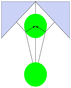
Figure 1: A Nonconvex Generalized Fermat-Torricelli Problem.

Example 4.5

(nonconvex generalized Fermat-Torricelli problem on the plane). In the setting of Corollary 4.4, let $\Omega_{1}$ be the ball centered at $c_{1}:=(0,-2)$ with radius $r=1$, let $\Omega_{2}$ be the ball centered at $c_{2}:=(0,-6)$ with the same radius $r=1$, and let $\Omega_{3}$ be a nonconvex set defined by

$$\Omega_{3}:=\big{\{}(x_{1},x_{2})\in I\!\!R^{2}\big{|}\;x_{2}\geq-|x_{1}|\big{\}}$$ (4.15)

as depicted on Figure 1. By Proposition 4.1 there is an optimal solution to this problem. Applying then Corollary 4.4, all the assumptions of which are satisfied, we find two points lying on the boundary of $\Omega_{1}$ and denoted by $u$ and $v$ such that $[c_{1},u]$ is the angle bisector for the angle formed by the lines $uc_{2}$ and $up_{u}$, where $p_{u}$ is the projection of $u$ to $\Omega_{3}$, while $[v,c_{1}]$ is the angle bisector for the angle formed by the lines $vc_{2}$ and $vp_{v}$. These two points satisfy (i) of Corollary 4.4 and they are actually the optimal solutions to the problem under consideration. It is not hard to find $u$ and $v$ numerically; we get $u=(-0.8706,-2.4920)$ and $v=(0.8706,-2.4920)$ up to five significant digits, with the optimal value of the problem equal to 3.7609.

We continue now by considering the generalized Fermat-Torricelli problem (1.3) with convex target set $\Omega_{i}$ as $i=1,\ldots,n$ in Banach spaces. In this case we derive necessary and sufficient optimality conditions for Fermat-Torricelli points.

It follows from Theorem 3.1 and Theorem 3.3 that in the case of convex sets $\Omega_{i}$ with $\Pi^{F}_{\Omega_{i}}(x;\Omega_{i})\neq\emptyset$ as $x\notin\Omega_{i}$ and $0\in F$ we have the equalities

$$A_{i}(x)=-\partial\rho_{F}(\omega-x)\cap N(\omega;\Omega_{i})\;\mbox{ for any }\;x\in X\;\mbox{ and }\;\omega\in\Pi^{F}_{\Omega_{i}}(x;\Omega_{i})$$ (4.16)

for the sets $A_{i}(x)$ defined in (4.1), where the subdifferential and normal cone are explicitly computed by formulas (2.1) and (2.3) of convex analysis. Here is a characterization of Fermat-Torricelli points for convex problems.

Theorem 4.6

(necessary and sufficient conditions for generalized Fermat-Torricelli points of convex problems in Banach spaces). Let all the target sets $\Omega_{i}$ be convex, let $0\in\mbox{\rm int}\,F$ for problem (1.3) formulated in a Banach space $X$, and let $\bar{x}\in X$ be such that $\Pi^{F}_{\Omega_{i}}(\bar{x})\neq\emptyset$ whenever $\bar{x}\notin\Omega_{i}$ as $i=1,\ldots,n$. Then condition (4.3) with the sets $A_{i}(\bar{x})$ defined in (4.16) is necessary and sufficient for optimality of $\bar{x}$ in this problem.

Proof. As mentioned above, the convexity of all the sets $\Omega_{i}$ implies the convexity of the cost function $T(x)$ in problem (1.3). By the generalized Fermat rule (2.2) for convex functions we get the inclusion $0\in\partial T(\bar{x})$ as a necessary and sufficient conditions for optimality of $\bar{x}\in X$ in (1.3). Since all the functions $T^{F}_{\Omega_{i}}(\cdot)$ are locally Lipschitzian under the interiority assumption on the dynamics $F$, the convex subdifferential sum rule of Theorem 2.1 ensures that the latter inclusion is equivalent to

$$0\in\sum_{i=1}^{n}\partial T^{F}_{\Omega_{i}}(\bar{x}).$$ (4.17)

Applying now relationship (4.2) and equality (3.4) of Theorem 3.1 in the in-set case as well as Theorem 3.3 in the out-of-set case, we conclude that $\partial T^{F}_{\Omega_{i}}(\bar{x})=A_{i}(\bar{x})$ as $i=1,\ldots,n$. Thus inclusion (4.17) is equivalent to (4.3), and the latter is necessary and sufficient for optimality of $\bar{x}$ in the convex Fermat-Torricelli problem (1.3). $\hfill\triangle$

The following consequence of Theorem 4.6 provides an explicit characterization of Fermat-Torricelli points in the convex Steiner-type extension (1.4) of the classical problem in the Hilbert space setting. In this case we use formula (4.9) for constructing the sets $A_{i}(\bar{x})$, which reduce to singletons if $\bar{x}\notin\Omega_{i}$ and are computed explicitly by (2.3) if $\bar{x}\in\Omega_{i}$.

Corollary 4.7

(characterization of optimal solutions to the convex Steiner-type extension of the Fermat-Torricelli problem in Hilbert spaces). Let $X$ be a Hilbert space, and let all the sets $\Omega_{i}$ in (1.4) be convex. Then condition (4.3) with $A_{i}(\bar{x})$ computed in (4.9) is necessary and sufficient for optimality of $\bar{x}\in X$ in problem (1.4).

Proof. It follows from Theorem 4.6 due the fact that the sets $A_{i}(\bar{x})$ from (4.1) reduce to those in (4.9) as proved in Theorem 4.3 and due to the projection nonemptiness $\Pi(\bar{x};\Omega_{i})\neq\emptyset$ for any $\bar{x}\in X$ and $i=1,\ldots,n$ in the setting under consideration. $\hfill\triangle$

Note that, in contrast to problem (1.4) addressed in Corollary 4.7, the characterization of generalized Fermat-Torricelli points for problem (1.3) obtained in Theorem 4.6 depends on the dynamics $F$ and clearly determines different solutions for the same targets sets $\Omega_{i}$ while different dynamics sets $F$. For example, consider the case of the three singletons $\Omega_{1}:=\{(-1,0)\}$, $\Omega_{2}:=\{(0,1)\}$, and $\Omega_{3}:=\{(1,0)\}$ on the plane $I\!\!R^{2}$. Then Corollary 4.7 gives us the unique optimal solution $(0,1/\sqrt{3})$ to the corresponding problem (1.4), while for $F=[-1,1]\times[-1,1]$ and the same sets $\Omega_{i}$, $i=1,2,3$, we have the unique optimal solution $(0,1)$ to the generalized Fermat-Torricelli problem (1.3) with these sets $F$ and $\Omega_{i}$.

Let us present a simple application of Corollary 4.7 to a version of the generalized Fermat-Torricelli problem (1.4) for finitely many disjoint closed intervals of the real line.

Proposition 4.8

(Fermat-Torricelli problem for closed intervals of the real line). Consider problem (1.4) with the sets $\Omega_{i}$ given by $n$ disjoint closed intervals $[a_{i},b_{i}]\subset I\!\!R$ as $i=1,\ldots,n$, where $a_{1}\leq b_{1}<a_{2}\leq b_{2}<\ldots<a_{n}\leq b_{n}$. The following hold:

(i) If $n=2k+1$, then any point of the interval $[a_{k+1},b_{k+1}]$ $($the mid interval$)$ is an optimal solution to the problem under consideration.

(ii) If $n=2k$, then any point of the interval $[b_{k},a_{k+1}]$ is an optimal solution to the problem under consideration.

Proof. Let $\varphi(x):=\mbox{d}(x;\Omega)$ with $\Omega=[a,b]$. It is easy to compute (as, e.g., a particular case of Theorem 3.3) the subdifferential of $\varphi$ by:

$$\partial\varphi(\bar{x})=\left\{\begin{array}[]{ll}\{0\}&\mbox{ if }\;a<\bar{x}<b,\\ ${\rm[-1,0]}$&\mbox{ if }\;\bar{x}=a,\\ ${\rm[0,1]}$&\mbox{ if }\;\bar{x}=b,\\ ${\rm\{-1\}}$&\mbox{ if }\;\bar{x}<a,\\ ${\rm\{1\}}$&\mbox{ if }\;\bar{x}>b.\end{array}\right.$$

Consider first case (i) when $n=2k+1$, we get for any $\bar{x}\in[a_{k+1},b_{k+1}]$ the relationships

$$\sum_{i=1}^{k}\partial\mbox{d}(\bar{x};\Omega_{i})=\{k\},$$

$$\sum_{i=k+2}^{n}\partial\mbox{d}(\bar{x};\Omega_{i})=\{-k\},$$

$$\mbox{and }0\in\partial\mbox{d}(\bar{x};\Omega_{k+1}).$$

The latter implies that $0\in\sum_{i=1}^{n}\partial\mbox{d}(\bar{x};\Omega_{i})$, which ensures by Corollary 4.7 that $\bar{x}$ is an optimal solution to the problem under consideration. Taking further any $\bar{x}\notin[a_{k+1},b_{k+1}]$, we get by the above calculation that $0\notin\sum_{i=1}^{n}\partial\mbox{d}(\bar{x};\Omega_{i})$ and hence learn from the characterization of Corollary 4.7 that such a number $\bar{x}$ cannot be an optimal solution to the problem. The even case of $n$ in (ii) is treated similarly. $\hfill\triangle$

Another application of Corollary 4.7 provides complete characterizations of Fermat-Torricelli points for the convex problem (1.4) with $n=3$ in Hilbert spaces. Note that in this case, due the projection uniqueness, we have

$$A_{i}(\bar{x})=a_{i}:=\Big{\{}\dfrac{\bar{x}-\Pi(\bar{x};\Omega_{i})}{\mbox{d}(\bar{x};\Omega_{i})}\Big{\}},\quad\bar{x}\notin\Omega_{i},$$ (4.18)

for the sets $A_{i}(\bar{x})$ defined in (4.9).

Proposition 4.9

(characterizations of generalized Fermat-Torricelli points for three convex sets in Hilbert spaces). Let $X$ be a Hilbert space, and let $\Omega_{1},\Omega_{2},\Omega_{3}$ be pairwise disjoint convex subsets of $X$. Then $\bar{x}\in X$ is an optimal solution to problem (1.4) generated by these sets if and only if one of the conditions (i) and (ii) of Corollary 4.4 is satisfied, where the vectors $a_{i}$, $i=1,2,3$, are defined in (4.18), and where the normal cone $N(\bar{x};\Omega_{1})$ in (4.11) is computed by (2.3).

Proof. The necessity part of the proposition follows from Corollary 4.4 by the observations that the convex problems under consideration is well posed at $\bar{x}$ and that $\emptyset\neq\Pi(\bar{x};\Omega_{i})$ is a singleton for any $i=1,2,3$. The sufficiency part of the proposition can be derived from Corollary 4.7 by the arguments developed in the proof of Corollary 4.4. $\hfill\triangle$

Finally in this section, we illustrate the application of Proposition 4.9 to some particular problems of Fermat-Torricelli type formulated on the plane.

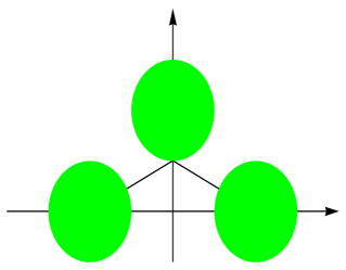
Figure 2: A Convex Generalized Fermat-Torricelli Problem.

Example 4.10

(convex generalized Fermat-Torricelli problems on the plane). Let the sets $\Omega_{1}$, $\Omega_{2}$, and $\Omega_{3}$ in problem (1.4) are closed balls in $I\!\!R^{2}$ of radius $r=1$ centered at the points $(0,2)$, $(-2,0)$, and $(2,0)$, respectively; see Figure 2. We can easily see that the point $(0,1)\in\Omega_{1}$ satisfies all the conditions in Proposition 4.9(i), and hence it is an optimal solution (in fact a unique one) to this problem.

More generally, consider problem (1.4) in $I\!\!R^{2}$ generated by three arbitrary pairwise disjoint disks denoted by $\Omega_{i}$, $i=1,2,3$. Let $c_{1}$, $c_{2}$, and $c_{3}$ be the centers of the disks. Assume first that either the line segment $[c_{2},c_{3}]\in I\!\!R^{2}$ intersects $\Omega_{1}$, or $[c_{1},c_{3}]$ intersects $\Omega_{2}$, or $[c_{1},c_{2}]$ intersects $\Omega_{3}$. It is not hard to check that any point of the intersections (say of the sets $\Omega_{1}$ and $[c_{2},c_{3}]$ for definiteness) is an optimal solution to the problem under consideration, since it satisfies the necessary and sufficient optimality conditions of Proposition 4.9(i). Indeed, if $\bar{x}$ is such a point, then $a_{2}$ and $a_{3}$ from (4.18) are unit vectors with $\langle a_{2},a_{3}\rangle=-1$ and $-a_{2}-a_{3}=0\in N(\bar{x};\Omega_{1})$.

If the above intersection assumptions are violated, we define three points $q_{1},q_{2}$, and $q_{3}$ as follows. Let $u$ and $v$ be the intersections of $[c_{1},c_{2}]$ and $[c_{1},c_{3}]$ with the boundary of the disk centered in $c_{1}$. Then we can see that there is a unique point $q_{1}$ on the minor curve generated by $u$ and $v$ such that the measures of angle $c_{1}q_{1}c_{2}$ and $c_{1}q_{1}c_{3}$ are equal. The points $q_{2}$ and $q_{3}$ are defined similarly. Proposition 4.9 yields that whenever the angle $c_{2}q_{1}c_{3}$, or $c_{1}q_{2}c_{3}$, or $c_{2}q_{3}c_{1}$ equals or exceeds $120^{\circ}$ (say the angle $c_{2}q_{1}c_{3}$ does), then the point $\bar{x}:=q_{1}$ is an optimal solution to the problem under consideration. Indeed, in this case $a_{2}$ and $a_{3}$ from (4.18) are unit vectors with $\langle a_{2},a_{3}\rangle\leq-1/2$ and $-a_{2}-a_{3}\in N(\bar{x};\Omega_{1})$ because the vector $-a_{2}-a_{3}$ is orthogonal to $\Omega_{1}$.

If none of these angles equals or exceeds $120^{\circ}$, there is a point $q$ not belonging to $\Omega_{i}$ as $i=1,2,3$ such that the angles $c_{1}qc_{2}=c_{2}qc_{3}=c_{3}qc_{1}$ are of $120^{\circ}$, and $q$ is an optimal solution to the problem. Observe that in this case the point $q$ is also a unique optimal solution to the classical Fermat-Torricelli problem determined by the points $c_{1},c_{2}$, and $c_{3}$.

5 Generalized Fermat-Torricelli Problem in Convex Settings: Numerical Aspects

The concluding section of the paper is devoted to some numerical aspects of solving the generalized Fermat-Torricelli problem (1.3) and its concretizations for the case of $n$ convex target sets in finite-dimensional spaces. Based on the subgradient method in convex optimization and the subdifferential calculus results discussed in Sections 2 and 3, we develop a first-order algorithm of solving a general convex problem (1.3) and present some of its specifications and implementations.

Theorem 5.1

(subgradient algorithm for the generalized Fermat-Torricelli problem). Let $\Omega_{i}$, $i=1,\ldots,n$, be convex subsets of a finite-dimensional Euclidean space $X$, let $0\in\mbox{\rm int}\,F$, and let $S\neq\emptyset$ be the set of optimal solutions to problem (1.3). Picking a sequence $\{\alpha_{k}\}$ as $k\in I\!\!N$ of positive numbers and a starting point $x_{1}\in X$, consider the algorithm

$$x_{k+1}=x_{k}-\alpha_{k}\sum_{i=1}^{n}v_{ik},\quad k=1,2,\ldots,$$ (5.1)

with an arbitrary choice of vectors

$$v_{ik}\in-\partial\rho(\omega_{ik}-x_{k})\cap N(\omega_{ik};\Omega_{i})\;\mbox{ for some }\;\omega_{ik}\in\Pi^{F}_{\Omega_{i}}(x_{k})\;\mbox{ if }\;x_{k}\notin\Omega_{i}$$ (5.2)

and $v_{ik}=0$ otherwise. Assume that

$$\sum_{k=1}^{\infty}\alpha_{k}=\infty\;\mbox{ and }\;\ell^{2}:=\sum_{k=1}^{\infty}\alpha_{k}^{2}<0.$$ (5.3)

Then the iterative sequence $\{x_{k}\}$ in (5.2) converges to an optimal solution for problem (1.3) and the value sequence

$$V_{k}:=\min\big{\{}T(x_{j})\big{|}\;j=1,\ldots,k\big{\}}$$ (5.4)

converges to the optimal value $\widehat{V}$ in this problem. Furthermore, we have the estimate

$$V_{k}-\widehat{V}\leq\dfrac{{\rm{d}}(x_{1};S)^{2}+L^{2}\ell^{2}}{2\sum_{i=1}^{k}\alpha_{k}},$$

where $0\leq L<\infty$ is a Lipschitz constant of the function $T(\cdot)$ from (1.3) on $X$.

Proof. As mentioned above, the value function $T(\cdot)$ in (1.3) is convex and globally Lipschitzian on $X$. By Theorem 3.1 and Theorem 3.3 the convex subdifferential of the minimal time functions (1.1) at $x_{k}$ is computed by

$$\partial T^{F}_{\Omega_{i}}(x_{k})=\left\{\begin{array}[]{ll}N(x_{k};\Omega_{i})\cap\big{\{}v\in X\big{|}\;\sigma_{F}(-v)\leq 1\big{\}}&\mbox{if }\;x_{k}\in\Omega_{i},\\ \\ N(\omega_{ik};\Omega_{i})\cap\big{[}-\partial\rho(\omega_{ik}-x_{k})\big{]}&\mbox{ if }\;x_{k}\notin\Omega_{i},\end{array}\right.$$ (5.8)

where $\omega_{ik}\in\Pi^{F}_{\Omega_{i}}(x_{k})$ is any generalized projection vector, $i\in\{1,\ldots,n\}$, and $k\in I\!\!N$. Recalling now the subgradient algorithm for minimizing the convex function $T(\cdot)$, we have

$$x_{k+1}=x_{k}-\alpha_{k}\sum_{i=1}^{n}v_{k}\;\mbox{ with }\;v_{k}\in\partial T(x_{k}),\quad 1,2,\ldots.$$ (5.9)

The convex subdifferential sum rule of Theorem 2.1 provides the representation

$$v_{k}=\sum_{i=1}^{n}v_{ik}\;\mbox{ with }\;v_{ik}\in\partial T^{F}_{\Omega_{i}}(x_{k})$$

of the subgradient $v_{k}$ in (5.9). Substituting the latter into (5.9) gives us algorithm (5.1) with $v_{ik}$ satisfying (5.2). Employing now the well-known results on the subgradient method for convex functions in the so-called “square summable but not summable case” (see, e.g., [2]), we arrive at the conclusions of the theorem under the conditions in (5.3). $\hfill\triangle$

Note that, using the above arguments, we can similarly apply to the generalized Fermat-Torricelli problem the subgradient method for convex optimization in the other cases considered in [2] with the corresponding replacements of the convergence conditions (5.3).

Let us present a useful consequence of Theorem 5.1 in the setting of (1.3) when the Minkowski gauge (3.5) is differentiable everywhere but the origin; this holds, e.g., for the distance function (1.2). In the case under consideration we denote

$$g_{F}(x):=\left\{\begin{array}[]{ll}\nabla\rho_{F}(x)&\mbox{if }\;x\neq 0,\\ \\ 0&\mbox{if }\;x=0.\end{array}\right.$$ (5.10)

Corollary 5.2

(subgradient algorithm under smoothness assumptions). In the setting of Theorem 5.1, assume in addition that the Minkowski gauge $\rho_{F}(\cdot)$ is differentiable at every point $X\setminus\{0\}$. Picking a sequence of positive numbers $\{\alpha_{k}\}$ satisfying conditions (5.3) and given a starting point $x_{1}\in X$, form the algorithm

$$x_{k+1}=x_{k}+\alpha_{k}\sum_{i=1}^{n}g_{F}(\omega_{ki}-x_{k}),$$ (5.11)

where $\omega_{ik}\in\Pi^{F}_{\Omega_{i}}(x_{k})$ is an arbitrary projection vector. Then all the conclusions of Theorem 5.1 hold true for algorithm (5.11).

Proof. Fix $i\in\{1,\ldots,n\}$ and $k\in I\!\!N$. When $x_{k}\notin\Omega_{i}$ we have $\omega_{ik}-x_{k}\neq 0$ for any $\omega_{ik}\in\Pi^{F}_{\Omega_{i}}(x_{k})$. Hence $\partial\rho_{F}(w_{ik}-x_{k})=\nabla\rho_{F}(x_{k}-\omega_{ik})=g_{F}(\omega_{ik}-x_{k})$ by (5.10), and the intersection $-\partial\rho_{F}(\omega_{k}-x_{ik})\cap N(\omega_{ik};\Omega_{i})$ reduces to the singleton $\{-g_{F}(\omega_{ik}-x_{k})\}$, which we take for $v_{ik}$ in Theorem 5.1 when $x_{k}\notin\Omega_{i}$. In the other hand, for $x_{k}\in\Omega_{i}$ we get

$$v_{ik}:=0=-g_{F}(0)=-g_{F}(\omega_{ik}-x_{k}).$$

Thus algorithm (5.11) in both cases agrees with (5.1) under the assumptions made.$\hfill\triangle$

We have a further specification of algorithm (5.11) for the convex problem (1.4).

Corollary 5.3

(subgradient algorithm for convex Steiner-type extensions). Consider problem (1.4) with convex sets $\Omega_{i}$, $i=1,\ldots,n$, in a finite-dimensional Euclidean space $X$. Given a sequence $\{\alpha_{k}\}$ of positive numbers satisfying (5.3) and a starting point $x_{1}\in X$, form algorithm (5.11) with $g_{F}(\cdot)$ computed by

$$g_{F}(\omega_{ki}-x_{k})=\left\{\begin{array}[]{ll}\dfrac{\Pi(x_{k};\Omega_{i})-x_{k}}{{\rm{d}}(x_{k};\Omega_{i})}&\mbox{ if }\;x_{k}\notin\Omega_{i},\\ \\ 0&\mbox{ if }\;x_{k}\in\Omega_{i}.\end{array}\right.$$ (5.15)

Then all the conclusions of Theorem 5.1 are satisfied for this algorithm.

Proof. Follows from Corollary 5.2 with $\rho_{F}(x)=\|x\|$ and $\nabla\rho_{F}(x)=\dfrac{x}{\|x\|}$ if $x\neq 0$. $\hfill\triangle$

Now we consider some examples of implementing the above subgradient algorithms to the numerical solution of particular versions of the generalized Fermat-Torricelli problem.

Example 5.4

(Fermat-Torricelli problem for disks). Consider the Steiner-type extension (1.4) of the Fermat-Torricelli problem for pairwise disjoint circular disks in $I\!\!R^{2}$. Let $c_{i}=(a_{i},b_{i})$ and $r_{i}$, $i=1,\ldots,n$, be the centers and the radii of the disks under consideration. The subgradient algorithm of Corollary 5.3 is written in this case as

$$x_{k+1}=x_{k}-\alpha_{k}\sum_{i=1}^{n}q_{ik},$$ (5.16)

where the quantities $q_{ik}$ are given by

$$q_{ik}=\left\{\begin{array}[]{ll}0&\mbox{if }\;\|x_{k}-c_{i}\|\leq r_{i},\\ \\ \displaystyle\frac{x_{k}-c_{i}}{\|x_{k}-c_{i}\|}&\mbox{if }\;\|x_{k}-c_{i}\|>r_{i}.\end{array}\right.$$

The corresponding quantities $V_{k}$ are evaluated by formula (5.4) with

$$T(x_{j})=\sum_{i=1,\;x_{j}\notin\Omega_{i}}^{n}\big{(}\|x_{j}-c_{i}\|-r_{i}\big{)}.$$

Writing a MATLAB program, we can compute by the above expressions the values of $x_{k}$ and $V_{k}$ for any number of disks and iterations. This allows us, in particular, to examine the convergence of the algorithm in various settings. The following table shows the results from the implementation of the above algorithm for three circles with centers $(-2,0)$, $(0,2)$, and $(2,0)$ and with the same radius $r=1$. The presented calculations are performed for the sequence $\alpha_{k}=1/k$ satisfying (5.3) and the starting point $x_{1}=(5,7)$.

MATLAB RESULT
$k$	$x_{k}$	$V_{k}$
10	(0.6224, 1.1995)	2.7243
100	(0.0552, 0.9984)	2.4741
1,000	(0.0047, 0.9995)	2.4721
10,000	(0.0004, 0.9999)	2.4721
100,000	(0.0000, 1.0000)	2.4721
1,000,000	(0.0000, 1.0000)	2.4721

Observe that the numerical results obtained in this case are consistent with the theoretical ones given in Proposition 4.9.

For four disks centered at $(0,0),(2,2),(1,0)$, and $(2,-2)$ and the same radius $r=1/4$, the MATLAB program gives us the optimal point $(0.8453,-0.0000)$ and the optimal value $4.7141$. For five disks centered at $(-1,0),(-1,1),(0,2),(1,1)$, and $(1,0)$ with radius $r=1/2$, we get the optimal solution $(0.0000,0.8505)$ and the optimal value equal to $3.2973$.

Next we apply the subgradient algorithm (5.11) to the Steiner-type extension (1.4) of the Fermat-Torricelli problem for the case of squares $\Omega_{i}$, which is significantly different from the case of disks in Example 5.4.

Example 5.5

(Fermat-Torricelli problem for squares). Consider problem (1.4) generated by pairwise disjoint squares $\Omega_{i}$, $i=1,\ldots,n$, of right position in $I\!\!R^{2}$, i.e., such that the sides of each square are parallel to the $x$-axis or the $y$-axis; see Figure 3. The center of a square is the intersection of its two diagonals, and its radius equals one half of the side. Let $c_{i}=(a_{i},b_{i})$ and $r_{i}$, $i=1,\ldots,n$, be the centers and the radii of the squares under considerations. Then the vertices of the $i$th square are denoted by $v_{1i}=(a_{i}+r_{i},b_{i}+r_{i})$, $v_{2i}=(a_{i}-r_{i},b_{i}+r_{i})$, $v_{3i}=(a_{i}-r_{i},b_{i}-r_{i})$, and $v_{4i}=(a_{i}+r_{i},b_{i}-r_{i})$.

Given a starting point $x_{1}$ and a sequence $\{\alpha_{k}\}$ satisfying the conditions in (5.3), the subgradient algorithm of Corollary 5.3 can be written in form (5.16), where $x_{k}=(x_{1k},x_{2k})$ and where the quantities $q_{ik}$ are computed as follows:

$$q_{ik}=\left\{\begin{array}[]{ll}0&\mbox{ if }\;|x_{1k}-a_{i}|\leq r_{i}\;\mbox{ and }\;|x_{2k}-b_{i}|\leq r_{i},\\ \\ \dfrac{x_{k}-v_{1i}}{\|x_{k}-v_{1i}\|}&\mbox{ if }\;x_{1k}-a_{i}>r_{i}\;\mbox{ and }\;x_{2k}-b_{i}>r_{i},\\ \\ \dfrac{x_{k}-v_{2i}}{\|x_{k}-v_{2i}\|}&\mbox{ if }\;x_{1k}-a_{i}<-r_{i}\;\mbox{ and }\;x_{2k}-b_{i}>r_{i},\\ \\ \dfrac{x_{k}-v_{3i}}{\|x_{k}-v_{3i}\|}&\mbox{ if }\;x_{1k}-a_{i}<-r_{i}\;\mbox{ and }\;x_{2k}-b_{i}<-r_{i},\\ \\ \dfrac{x_{k}-v_{3i}}{\|x_{k}-v_{4i}\|}&\mbox{ if }\;x_{1k}-a_{i}>r_{i}\;\mbox{ and }\;x_{2k}-b_{i}<-r_{i},\\ \\ (0,1)&\mbox{ if }\;|x_{1k}-a_{i}|\leq r_{i}\;\mbox{ and }\;x_{2k}-b_{i}>r_{i},\\ \\ (0,-1)&\mbox{ if }\;|x_{1k}-a_{i}|\leq r_{i}\;\mbox{ and }\;x_{2k}-b_{i}<-r_{i},\\ \\ (1,0)&\mbox{ if }\;x_{1k}-a_{i}>r_{i}\;\mbox{ and }\;|x_{2k}-b_{i}|\leq r_{i},\\ \\ (-1,0)&\mbox{ if }\;x_{1k}-a_{i}<-r_{i}\;\mbox{ and }\;|x_{2k}-b_{i}|\leq r_{i}\end{array}\right.$$

for all $i\in\{1,\ldots,n\}$ and $k\in I\!\!N$, with the corresponding value sequence $V_{k}$ defined by (5.4).

Considering the implementation of the above algorithm for three squares with centers $(-2,0)$, $(0,2)$, and $(2,0)$ and with the same radius $r=1/2$, we arrive at the optimal solution $(0,1.3660)$ and the optimal value $3.5981$. At the same time applying the theoretical results of Corollary 5.3 to this case gives us the exact optimal solution $(0,\dfrac{\sqrt{3}+1}{2})$ with the optimal value $\dfrac{2+3\sqrt{3}}{2}$, which are consistent with the numerical calculation.

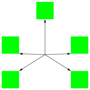
Figure 3: A Generalized Fermat-Torricelli Problem for Five Squares.

For five squares with centers at $(-1,0),(-1,1),(0,2),(1,1)$, and $(1,0)$ and the same radius $r=1/4$ we get by the subgradient algorithm the optimal solution $(0.0000,0.7242)$ with the optimal value equal to $4.3014$. However, it does not seem to be an easy exercise to solve the above problem theoretically by using Corollary 5.3.

Let us finally illustrate applications of the subgradient algorithm of Theorem 5.1 to solving the generalized Fermat-Torricelli problem (1.3) formulated via the minimal time function (1.1) with non-ball dynamics. For definiteness we consider the dynamics $F$ given by the square $[-1,1]\times[-1,1]$ on the plane. In this case the corresponding Minkowski gauge (3.5) is given by the formula

$$\rho_{F}(x_{1},x_{2})=\max\big{\{}|x_{1}|,|x_{2}|\big{\}}.$$ (5.18)

Note that the function $\rho_{F}(\cdot)$ fails to be differentiable at every nonzero point of $I\!\!R^{2}$, so we have to relay on the subgradient algorithm of Theorem 5.1 but not of its corollaries above. Observe also that to implement algorithm (5.1) we need to know just one element $v_{ik}$ from the set on the right-hand side of (5.2) for each $i\in\{1,\ldots,n\}$ and $k\in I\!\!N$. By Theorem 3.3 the latter set agrees with the subdifferential of the minimal time function $T^{F}_{\Omega_{i}}(x_{k})$.

In the following proposition we compute a subgradient of the minimal time function (1.1) generated by the Minkowski gauge (5.18) and a square target in $I\!\!R^{2}$, which is used then to construct a subgradient algorithm to solve the corresponding Fermat-Torricelli problem.

Proposition 5.6

(subgradients of minimal time functions with square dynamics and targets). Let $F=[-1,1]\times[-1,1]$, and let $\Omega$ be a square of right position in $I\!\!R^{2}$ centered at $c=(a,b)$ with radius $r>0$. Then a subgradient $v(\bar{x}_{1},\bar{x}_{2})\in\partial T^{F}_{\Omega}(\bar{x}_{1},\bar{x}_{2})$(not necessarily uniquely defined) of the minimal time function $T^{F}_{\Omega}(x_{1},x_{2})$ at $(\bar{x}_{1},\bar{x}_{2})$ is computed by

$$v(\bar{x}_{1},\bar{x}_{2})=\left\{\begin{array}[]{ll}(1,0)&\mbox{if }\;|\bar{x}_{2}-b|\leq\bar{x}_{1}-a,\;\bar{x}_{1}>a+r,\\ \\ (-1,0)&\mbox{if }\;|\bar{x}_{2}-b|\leq a-\bar{x}_{1},\;\bar{x}_{1}<a-r.\\ \\ (0,1)&\mbox{if }\;|\bar{x}_{1}-a|\leq\bar{x}_{2}-b,\;\bar{x}_{2}>b+r,\\ \\ (0,-1)&\mbox{if }\;|\bar{x}_{1}-a|\leq b-\bar{x}_{2},\;\bar{x}_{2}<b-r,\\ \\ 0&\mbox{if }\;(\bar{x}_{1},\bar{x}_{2})\in\Omega.\end{array}\right.$$ (5.28)

Proof. It is ease to see that the minimal time function (1.1) admits the representation

$$T^{F}_{\Omega}(x)=\inf_{\omega\in\Omega}\rho_{F}(x;\Omega).$$

This implies by (5.18) and the above structure of $\Omega$ that

$$T^{F}_{\Omega}(x_{1},x_{2})=\left\{\begin{array}[]{ll}x_{1}-(a+r)&\mbox{if }\;|x_{2}-b|\leq x_{1}-a,\;x_{1}>a+r,\\ \\ (a-r)-x_{1}&\mbox{if }\;|x_{2}-b|\leq a-x_{1},\;x_{1}<a-r,\\ \\ x_{2}-(b+r)&\mbox{if }\;|x_{1}-a|\leq x_{2}-b,\;x_{2}>b+r,\\ \\ (b-r)-x_{2}&\mbox{if }\;|x_{1}-a|\leq b-x_{2},\;x_{2}<b-r,\\ \\ 0&\mbox{if }\;(x_{1},x_{2})\in\Omega\end{array}\right.$$

for all $(x_{1},x_{2})\in I\!\!R^{2}$. Applying to (5.18) the well-known subdifferential formula for maximum functions in convex analysis allows us to compute

$$\partial\rho_{F}(\bar{x}_{1},\bar{x}_{2})=\left\{\begin{array}[]{ll}\big{\{}(v_{1},v_{2})\in I\!\!R^{2}\;\big{|}\;|v_{1}|+|v_{2}|\leq 1\big{\}}&\mbox{if }\;(\bar{x}_{1},\bar{x}_{2})=(0,0),\\ \\ \{(0,1)\}&\mbox{if }\;|\bar{x}_{1}|<\bar{x}_{2},\\ \\ \{(0,-1)\}&\mbox{if }\;\bar{x}_{2}<-|\bar{x}_{1}|,\\ \\ \{(1,0)\}&\mbox{if }\;\bar{x}_{1}>|\bar{x}_{2}|,\\ \\ \{(-1,0)\}&\mbox{if }\;\bar{x}_{1}<-|\bar{x}_{2}|,\\ \\ \big{\{}(v_{1},v_{2})\in I\!\!R^{2}\;\big{|}\;|v_{1}|+|v_{2}|=1,\;v_{1}\geq 0,\;v_{2}\geq 0\big{\}}&\mbox{if }\;\bar{x}_{1}=\bar{x}_{2}>0,\\ \\ \big{\{}(v_{1},v_{2})\in I\!\!R^{2}\;\big{|}\;|v_{1}|+|v_{2}|=1,\;v_{1}\geq 0,\;v_{2}\leq 0\big{\}}&\mbox{if }\;\bar{x}_{1}=-\bar{x}_{2}>0,\\ \\ \big{\{}(v_{1},v_{2})\in I\!\!R^{2}\;\big{|}\;|v_{1}|+|v_{2}|=1,\;v_{1}\leq 0,\;v_{2}\leq 0\big{\}}&\mbox{if }\;\bar{x}_{1}=\bar{x}_{2}<0,\\ \\ \big{\{}(v_{1},v_{2})\in I\!\!R^{2}\;\big{|}\;|v_{1}|+|v_{2}|=1,\;v_{1}\leq 0,\;v_{2}\geq 0\big{\}}&\mbox{if }\;\bar{x}_{1}=-\bar{x}_{2}<0.\end{array}\right.$$

In this way we can check by Theorem 3.3 that the vector $v(\bar{x}_{1},\bar{x}_{2})$ is a subgradient of $T(\cdot,\cdot)$ at $(\bar{x},\bar{x}_{2})$, which completes the proof of the proposition. $\hfill\triangle$

Now we are able to implement the subgradient algorithm of Theorem 5.1 to the problem under consideration.

Example 5.7

(implementation of the subgradient algorithm). Consider the generalized Fermat-Torricelli problem (1.3) with the dynamics $F=[-1,1]\times[-1,1]$ and the square targets $\Omega_{i}$ of right position centered at $(a_{i},b_{i})$ with radii $r_{i}$ as $i=1,\ldots,n$. Given a sequence of positive numbers $\{\alpha_{k}\}$ satisfying (5.3) and a starting point $x_{1}$, construct the subgradient algorithm (5.1) for the iterations $x_{k}=(x_{1k},x_{2k})$ in Theorem 5.1, where the vectors $v_{ik}$ are computed by Proposition 5.6 as

$$v_{ik}=\left\{\begin{array}[]{ll}(1,0)&\mbox{if }\;|x_{2k}-b_{i}|\leq x_{1k}-a_{i}\;\mbox{ and }\;x_{1k}>a_{i}+r_{i},\\ \\ (-1,0)&\mbox{if }\;|x_{2k}-b_{i}|\leq a_{i}-x_{1k}\;\mbox{ and }\;x_{1k}<a_{i}-r_{i},\\ \\ (0,1)&\mbox{if }\;|x_{1k}-a_{i}|\leq x_{2k}-b_{i}\;\mbox{ and }\;x_{2k}>b_{i}+r_{i},\\ \\ (0,-1)&\mbox{if }\;|x_{1k}-a_{i}|\leq b_{i}-x_{2k}\;\mbox{ and }\;x_{2k}<b_{i}-r_{i},\\ \\ (0,0)&\mbox{otherwise.}\end{array}\right.$$

Implementing this algorithm for the case of three squares centered at $(-2,0)$, $(0,2)$, and $(2,0)$ with radius $r=1/2$, $\alpha_{k}=1/k$ and the initial point $(1,1)$, we arrive at an optimal solution $(0.0000,1.5000)$ and the optimal value equal to $3.0000$. For five squares centered at $(-1,0),(-1,1),(0,2),(1,1)$, and $(1,0)$ with radius $r=1/4$, we have the optimal solution $(0.0000,1.0000)$ and the optimal value equal to $3.7500$.

Acknowledgements. The authors are grateful to Jon Borwein, Michael Overton, and Boris Polyak for their valuable comments and references.

References

- [1] Andersen, K.D., Christiansen, A., Conn, A.R., Overton, M.L.: An efficient primal-dual interior-point method for minimizing a sum of Euclidean norms. SIAM J. Scient. Comp. 22, 243–262 (2000).
- [2] Bertsekas, D., Nedic, A., Ozdaglar, A.: Convex Analysis and Optimization. Athena Scientific, Boston (2003)
- [3] Bhattacharya, B.B.: On the Fermat-Weber point of a polynomial chain. ArHiv: 1004.2958v1 (2010)
- [4] Boltynski, V., Martini, H., Soltan, V.: Geometric Methods and Optimization Problems. Kluwer Academic, Dordrecht (1999)
- [5] Borwein, J.M., Vanderwerff, J.D.: Convex Functions: Characterizations, Constructions and Counterexamples. Cambridge University Press (2009)
- [6] Borwein, J.M., Zhu, Q.J.: Techniques of Variational Analysis. Springer, CMS Books in Mathematics 20, Springer, New York (2005)
- [7] Colombo, G., Goncharov, V.V., Mordukhovich, B.S.: Well-posedness of minimal time problem with constant dynamics in Banach spaces. Set-Valued Var. Anal., to appear (2010)
- [8] Colombo, G., Wolenski, P.R.: The subgradient formula for the minimal time function in the case of constant dynamics in Hilbert space. J. Global Optim. 28, 269 -282 (2004)
- [9] He, Y., Ng, K.F.: Subdifferentials of a minimum time function in Banach spaces. J. Math. Anal. Appl. 321, 896–910 (2006)
- [10] Kuhn, H.W.: Steiner’s problem revisited. Studies Math. 10, 52–70 (1974)
- [11] Martini, H., Swanepoel, K.J., Weiss, G.: The Fermat-Torricelli problem in normed planes and spaces. J. Optim. Theory Appl. 115, 283–314 (2002)
- [12] Mordukhovich, B.S.: Maximum principle in problems of time optimal control with nonsmooth constraints. J. Appl. Math. Mech. 40, 960–969 (1976)
- [13] Mordukhovich, B.S.: Variational Analysis and Generalized Differentiation, I: Basic Theory. Grundlehren Series (Fundamental Principles of Mathematical Sciences) 330, Springer, Berlin (2006)
- [14] Mordukhovich, B.S.: Variational Analysis and Generalized Differentiation, II: Applications. Grundlehren Series (Fundamental Principles of Mathematical Sciences) 331, Springer, Berlin (2006)
- [15] Mordukhovich, B.S., Nam, N.M.: Limiting subgradients of minimal time functions in Banach spaces. J. Global Optim. 46, 615–633 (2010)
- [16] Mordukhovich, B.S, Nam, N.M.: Subgradients of minimal time functions under minimal assumptions. J. Convex Anal., to appear (2010)
- [17] Phelps, R.R.: Convex Functions, Monotone Operators and Differentiability, 2nd edition. Lecture Notes Math. 1364, Springer, Berlin (1993)
- [18] Rockafellar, R.R., Wets, R.J-B.: Variational Analysis. Grundlehren Series (Fundamental Principles of Mathematical Sciences) 317, Springer, Berlin (1998)
- [19] Schirotzek, W.: Nonsmooth Analysis. Universitext, Springer, Berlin (2007)
- [20] Tan, T.V.: An extension of the Fermat-Torricelli problem. J. Optim. Theory Appl., published online (2010)
- [21] Weiszfeld, E.: On the point for which the sum of the distances to given points is minimum. Ann. Oper. Res. 167, 7–41 (2009). Translated from the French original [Tohoku Math. J. 43, 335–386 (1937)] and annotated by Frank Plastria.