Theoretical confirmation of Feynman’s hypothesis on the creation of circular vortices in Bose–Einstein condensates: III

Abstract

In two preceding papers (Infeld and Senatorski 2003 J. Phys.: Condens. Matter 15 5865, Senatorski and Infeld 2004 J. Phys.: Condens. Matter 16 6589) the authors confirmed Feynman’s hypothesis on how circular vortices can be created from oppositely polarized pairs of linear vortices (first paper), and then gave examples of the creation of several different circular vortices from one linear pair (second paper). Here in part III, we give two classes of examples of how the vortices can interact. The first confirms the intuition that the reconnection processes which join two interacting vortex lines into one and thus would increase the degree of entanglement of the vortex system, practically do not occur. The second shows that new circular vortices can also be created from pairs of oppositely polarized coaxial circular vortices. This seems to contradict the results for such pairs given in Koplik and Levine 1996 Phys. Rev. Lett. 76 4745.

, ,

1 Introduction

The discovery of superfluidity in helium II (⁴He and ³He) has aroused interest in boson liquids. This was recently renewed and intensified due to the experimental obtaining of Bose–Einstein condensates (BECs) in alkali metals. Especially interesting is the formation and time evolution of both curved and straight vortices which appear in these media [1, 2, 3].

In two preceding papers [4, 5], referred to as part I and part II, the time evolution of a pair of oppositely polarized linear vortices was examined. In part I, it was demonstrated that if such a pair is appropriately perturbed, a persistent set of identical circular vortices can be created. This was in full agreement with Feynman’s hypothesis [6] mentioned in the title. In part II, examples were given for the creation of several different circular vortices from one linear pair. In both cases, the BEC was examined within the commonly used Gross–Pitaevskii model [7, 8]. The authors checked that all circular vortices created during the evolution satisfied known relations between their velocities and radii [9].

Here, in part III, we examine the interaction of circular vortices with either linear ones, or else with other circular vortices of different radii, again within the Gross–Pitaevskii model. The results are compared with those of other authors [10]–[14].

2 Basic equations and initial conditions

In the present paper, as in parts I and II, we describe a one-component BEC by a single particle wavefunction of $N$ bosons of mass $m$ that obeys the nonlinear Schrödinger (NLS) type equation as formulated by Gross [7] and Pitaevskii [8],

$$\rmi\hbar\frac{\partial\psi}{\partial t}=-\frac{\hbar^{2}}{2m}\nabla^{2}\psi+W_{0}\psi|\psi|^{2},$$ (1)

where positive $W_{0}$ is the strength of the assumed $\delta$-function repulsive potential between bosons. Both linear pair and circular stationary vortex solutions are known, of which only the last ones were shown to be stable (see part I for references). Similarly, and for the same reasons as in parts I and II, we introduce dimensionless variables defined by the transformation

$$\psi\to\sqrt{\rho_{0}}\,\rme^{-\rmi\mu t/\hbar}\psi,\qquad\mathbf{x}\to\frac{\hbar}{\sqrt{2\mu m}}\mathbf{x},\qquad t\to\frac{\hbar}{2\mu}t,\qquad\mu=W_{0}\rho_{0},$$ (2)

where $\mu$ is the chemical potential and $\rho_{0}$ is the background mass density. Now, we obtain from (2) and (1)

$$2\rmi\frac{\partial\psi}{\partial t}=-\nabla^{2}\psi-\psi(1-|\psi|^{2}).$$ (3)

An initial condition used in parts I and II, was

$$\psi(t=0)=\frac{r_{1}r_{2}}{\sqrt{r_{1}^{2}+b^{2}}\sqrt{r_{2}^{2}+b^{2}}}\,\rme^{\rmi(\theta_{1}+\theta_{2})},$$ (4)

where ($y$ here has been interchanged with $z$)

$$r_{1}^{2}=(1-2U^{2})(x+a)^{2}+y^{2},\qquad r_{2}^{2}=(1-2U^{2})(x-a)^{2}+y^{2},$$ (5)

$$\tan\theta_{1,2}=\frac{y}{\sqrt{1-2U^{2}}(a\pm x)},$$ (6)

which is a model representing two oppositely polarized rectilinear vortices parallel to the $xz$ plane and moving along the $y$ axis. The constant $b$ was chosen such that the velocity of the two rectilinear vortices (along $y$) in the simulation would agree with $U$, from the theory, see [9], table 2. In spite of its simplicity, this model satisfies several criteria. The variable $x$ is scaled correctly, the wavefunction is zero at the centres of the two vortices, and far field behaviour is approximately correct (of the order of $1+O(1/r^{2}),r=\sqrt{x^{2}+y^{2}}$). (We have doubts about the formula of Jones and Roberts, see Appendix.) When the vortices are well separated, Fetters formula [15, 16] is recovered ($b^{2}\to 4$, and $U\to 0$ as $a\to\infty$).

In this paper, an initial condition for a circular vortex will be used. It will be described by formulae of similar form to (4)–(6), but with $x$ and $y$ replaced by

$$x\to{\rm sgn}(x-x_{0})\sqrt{(x-x_{0})^{2}+(z-z_{0})^{2}},\qquad y\to y-y_{0}.$$ (7)

The vortex in question will move along the $y$ axis with velocity close to $U$ taken from table 1 in [9], and the vortex lines ($\psi=0$) at $t=0$ will intersect the plane $z=z_{0}$ at two points: $x=x_{0}\mp a,\>y=y_{0}$.

It is clear that the accuracy of such a model will increase as we increase the radius $a$ of the circular vortex. However, as we observed in all considered cases, even for not very large values of $a$, the oscillations of the respective circular vortices during their motion were negligible.

The nonlinear Schrödinger equation in three dimensions (3) was numerically solved by using a discrete fast Fourier transform in $x$, $y$, and $z$ to calculate the space derivatives (pseudospectral algorithm), along with the leapfrog timestep. Calculations were performed in a box: $0\leq x\leq 2L_{x}$, $0\leq y\leq 2L_{y}$, $0\leq z\leq 2L_{z}$, with the number of mesh points $N_{x}=N_{z}=24$–$72$, and $N_{y}=96$–$192$. Periodic boundary conditions were assumed, and the timestep was determined from the numerical stability condition. The details of our calculations are described in [17].

3 Collisions of circular and almost linear vortices

Figures 1 and 2 present collisions of a circular vortex parallel to the $xz$ plane (of radius $r$) with an arc of another such vortex of much larger radius $R$ ($\gg r$). This arc, along with its periodic continuations to neighbouring periodicity boxes, models a linear vortex. (We have evidence that in this model, small disturbances of the initial condition for linear vortex, also involving small discontinuities in derivatives at the boundaries, only introduce small oscillations but do not change the main features of the evolution.) As the advection velocity (along the $y$ axis) of a circular vortex is a decreasing function of its radius (see e.g. figure 2 in Part I), the circular vortex of radius $r$ will be much faster than the “linear” one which, in the situation shown in figures 1 and 2, will imply their collision.

In figure 1, the $x$ components of the polarization vectors for the linear vortex and the neighbouring part of the circular one during collision have opposite signs, which locally resembles the situation analysed in Parts I and II, i.e. a pair of oppositely polarized rectilinear vortices. In figure 2, the pertinent signs are the same. Nevertheless, strange as it may seem, the result of the collision in both cases is topologically the same, i.e. a (distorted) circular vortex and a linear vortex. This is in contradiction to the description of the two above mentioned collisions given by Schwarz, see the second and third situation presented in figure 16 of [10]. In both these situations (in the Schwarz description) the reconnection occurs only at one of the crossing points and the result of the collision is topologically different from the initial state (one linear vortex only in the final state). It should be mentioned that different behaviour at the two crossing points (occurrence and lack of reconnection) is in fact also in contradiction to the results of Koplik and Levine [12] who examined the evolution (within the GP model) of two neighbouring rectilinear vortices for various angles between their vorticity vectors. Reconnection was demonstrated for angles between $90^{\circ}$ and $180^{\circ}$, and no reconnection for $45^{\circ}$. Thus, in the case of two rectilinear vortices, the angle $45^{\circ}$ implied the same behaviour as that for $0^{\circ}$. For the collisions shown in our figures 1 and 2, the angles between vorticity vectors at two intersection points are the same and one should not expect different behaviour there. Another question, however, is the applicability of the results of Koplik and Levine [12] to the collisions shown in figures 1 and 2, where one can only locally think in terms of rectilinear vortices during collision.

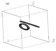
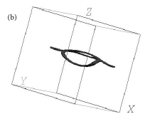
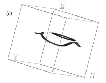
Figure 1: Collision of a circular vortex parallel to the $xz$ plane (of radius $r=8$) with an arc of another such vortex, but of much larger radius $R=400$, such that $R/r=50$. The distance between the “rectilinear” vortex and the axis of the circular one is 4. Consecutive times are: 0, 5$\tau$, 7$\tau$, $\tau=5.26$. Polarizations of the nearest segments of the approaching vortices are opposed.

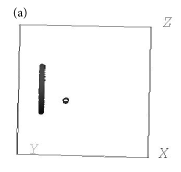
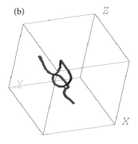
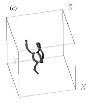
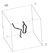
Figure 2: Collision similar to that shown in Fig. 1 but where the polarizations of the nearest segments of the colliding vortices agree. The radii are $r=18$, and $R=900$ ($R/r=50$), and the distance between the “rectilinear” vortex and the axis of the circular one is 9. Consecutive times are: $0$, $14\tau$, $18\tau$, $24\tau$, $\tau=6.11$. The first view is along the $x$ axis.

Here we pause for some comments. Firstly, we repeated the calculation but for the segment of the large circular vortex with opposite curvature. No difference between the results in both cases was observed. Secondly, we performed a calculation for a similar initial vortex configuration, but with both colliding circular vortices having comparable radii. We obtained essentially the same results (i.e. topologically, both results could be treated as identical). So the exact values of the radii of the colliding vortices are not important, if only the radius of one of the vortices is finite. Even more, a similar scenario of the collision of two circular oppositely polarized vortices is observed if the vortices have identical radii and their symmetry axes are parallel to each other but do not coincide. Again two reconnections at the crossing points and two distorted circular vortices after collision are obtained, see [14]. Note also that the initial conditions presented in figures 1 and 2 are symmetric with respect to the plane $x=L_{x}$ passing through both centres of colliding rings. This implies that this symmetry lasts during the evolution. This was the case in our results even if it is not obvious from figures 1 and 2.

As we have mentioned earlier, collisions as considered here were also investigated by K W Schwarz [10] who performed the first important step towards a formal description of the dynamics of vortices in BECs [10, 11]. Schwarz was able to explain many features of the vortex dynamics in these media, including the interaction with walls. In order to describe some simple observed effects, such as “avoiding collision” between parallel vortices and “attraction” by antiparallel ones, Schwarz introduced explicitly an “artificial force” acting between cores of neighbouring vortex lines. This made it possible to reach many detailed results, but also introduced the risk of some of these results being questionable.

The disagreement with our results has an important consequence. If in the course of the collision in question only one reconnection point appears, the two vortex lines join together into one vortex line and the degree of entanglement of the system of these lines increases. Our result, on the contrary, states that such coplanar collisions cannot increase the degree of entanglement and such a quick generation of vortex entanglement as showed Schwarz in his figure 4 in [11] cannot come about in this fashion.

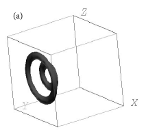
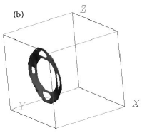
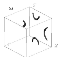
Figure 3: Coaxial collision of two oppositely polarized circular vortices parallel to the $xz$ plane with comparable radii, $R=8$, $r=4$ ($R/r=2$). The periodicity box has transverse dimensions ($2L_{x}=2L_{z}\equiv 2L$) comparable to the larger diameter $2R$ ($2L=28$, i.e. $L/R=1.75$). Consecutive times are: $0$, $4\tau$, $20\tau$, $\tau=5.23$.

4 Collisions of coaxial oppositely polarized circular vortices

In parts I and II the authors gave several examples of how circular vortices can be created from pairs of oppositely polarized rectilinear vortices perturbed sinusoidally in space. Here we will show that similar circular vortices can be created, if a circular vortex passes by another, oppositely polarized coaxial circular vortex of somewhat larger radius. This seems to contradict what Koplik and Levine say when considering a coaxial collision of oppositely polarized circular vortices of different radii, ([13], p. 4746):

“Two cases occur if two rings of different sizes approach on axis: if the ratio of radii is large, the rings simply leapfrog each other. If, however, the radii are comparable, one again sees annihilation similar to the equal-sized case, except that the partially overlapping rings continue to translate during the merger stage preceding annihilation.”

Different behaviour, resulting in reconnections and formation of circular vortices, should be possible if the the collision of the circular rings is somehow perturbed. In the case of rectilinear vortices, this perturbation was introduced externally. In the case of circular vortices, it could result from interaction (in the sense of Schwarz [10, 11]) of the colliding vortices with other circular vortices close by during the collision. Such situations are very probable in real condensates. In this paper, they have been modelled in the simplest possible way, i.e. by choosing the dimensions of the periodicity box in the plane parallel to the colliding vortices ($xz$ plane) to be comparable to the diameters of the colliding vortices. With this choice, the perturbation is due to the interaction of the colliding vortices with their neighbouring periodic images parallel to the $xz$ plane. There are four closest neighbours in the directions of the $x$ and $z$ axis, four further ones in the directions rotated by $45^{\circ}$ along the axis of the colliding vortices, still more along the $x$ and $z$ axis, etc. This evidently suggests that the number of circular vortices after collision should be a multiple of four. This prediction was confirmed by the results of our calculations as shown in figures 3–7.

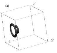
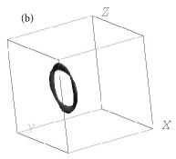
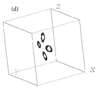
Figure 4: Coaxial collision of two circular vortices identical with those shown in Fig. 3 ($R/r=2$) but with somewhat larger periodicity box ($2L=42$, i.e. $L/R=2.625$). The formation of four smaller circular vortices after collision can be seen. Consecutive times are: $0$, $6\tau$, $7\tau$, $11\tau$, $\tau=6.75$.

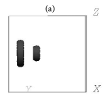
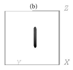
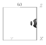
Figure 5: Coaxial collision of two circular vortices identical with those shown in Fig. 3 ($R/r=2$) but with a relatively large periodicity box ($2L=55$, i.e. $L/R\simeq 3.44$). No smaller circular vortices after collision can be seen. Consecutive times are: $0$, $6\tau$, $11\tau$, $\tau=6.29$.

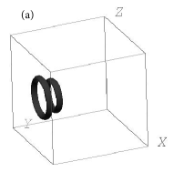
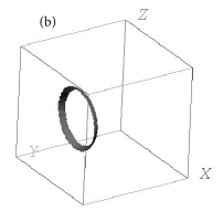
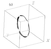
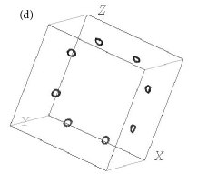
Figure 6: Coaxial collision of two oppositely polarized circular vortices parallel to the $xz$ plane with similar radii, $R=18$, $r=14$ ($R/r=1.3$). The periodicity box is not too large ($2L=84$, i.e. $L/R\simeq 2.33$). Consecutive times are: $0$, $8\tau$, $14\tau$, $18\tau$, $\tau=6.96$.

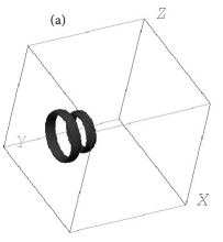
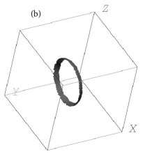
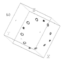
Figure 7: Coaxial collision of two oppositely polarized circular vortices with similar radii, identical with those shown in Fig. 6 ($R/r=1.3$) but with the periodicity box somewhat larger ($2L=100$, i.e. $L/R\simeq 2.78$). Consecutive times are: $0,12\tau,20\tau,\tau=5.35$. A “massive” production of smaller circular vortices continues. Note that in frame (c), the $xz$ plane is parallel to the page.

Figures 3–7 present head-on collisions of coaxially moving pairs of circular vortices with comparable radii. We first assume that the radius $R$ of the larger circular vortex is not too close to that of the smaller vortex, $r$, e.g. for $R/r=2$, see figures 3–5.

If the transverse box dimension is close enough to the size of the larger vortex, the interaction of the colliding pair with its images in the four closest neighbouring cells predominates over the main collision. As a result, the structure of the periodic vortex system changes, and four (distorted) circular vortices extending to the neighbouring cells are formed, see figure 3, where $L/R=1.75$. Only for more distant boundaries can we treat the interaction of the colliding pair with neighbouring pairs as merely a perturbation of the main collision. This perturbation can lead to the production of four smaller circular rings after collision, if the ratio $L/R$ is not too large, see figure 4, where $L/R=2.625$. Otherwise, the perturbation is too weak to switch on the reconnection, and the colliding rings pass through each other without decaying into smaller rings, see figure 5, where $L/R=3.45$. In all above cases ($R/r=2$), only the interaction with four nearest cells could be strong enough to turn on the reconnection.

The interaction with further cells can be significant if the larger ring is sufficiently close to the smaller one, e.g. for $R/r=1.3$, see figures 6 and 7, where respectively eight and twelve smaller circular vortices are formed after collision.

5 Summary

In parts I and II the authors demonstrated how circular vortices can be created from pairs of oppositely polarized line vortices and confirmed the $U(a)$ dependence, proving Feynman’s hypothesis. In this paper we present two alternate scenarios leading to the creation of smaller ring vortices from larger ones.

Appendix

Jones and Roberts [9] give formulas for the wavefunction in the far field for both the three dimensional case (circular vortex) and the two dimensional case (two counterstreaming line vortices). One might wish to compare their 2D model with our equation (4) in the far field. However, we have doubts about their derivation. They first linearize equation (3), obtaining in the far field ($z$ is interchanged with $y$ in our notation):

$$\psi_{\mathrm{i}}\sim-my[y^{2}+(1-2U^{2})x^{2}]^{-1},$$ (8)

$$\psi_{\mathrm{r}}\sim 1+mU[y^{2}-(1-2U^{2})x^{2}][y^{2}+(1-2U^{2})x^{2}]^{-2}.$$ (9)

They then find that the leading nonlinear term $-{\textstyle\frac{1}{2}}\psi_{\mathrm{i}}^{2}$ is at least of the same order as (9), $r^{-2}$, and simply tack it on:

$$\psi_{\mathrm{r}}\sim 1+m\{U[y^{2}-(1-2U^{2})x^{2}]-{\textstyle\frac{1}{2}}my^{2}\}[y^{2}+(1-2U^{2})x^{2}]^{-2}.$$ (10)

This is not proper procedure. The full, nonlinear equation (3) must be solved in the far field. Two inhomogeneous equations are obtained for $\psi_{\mathrm{i}}$ and $\psi_{\mathrm{r}}$ (the equation for $\psi_{\mathrm{i}}$ is free of $\psi_{\mathrm{r}}$). We add the good news that their other calculation is valid in 3D, the nonlinear correction being of higher order in $r^{-1}$ than the linear terms ($r^{-4}$ and $r^{-3}$ respectively).

References

References

- [1] Bewley G P, Lathrop D P, Sreenivasan K R 2006 Nature 441 588
- [2] Paoletti M S, Fisher M E, Lathtrop D P Physica D 2010 239 1367
- [3] Schwarzschild B July 2010 Physics Today 63 12
- [4] Infeld E and Senatorski A 2003 J. Phys.: Condens. Matter 15 5865
- [5] Senatorski A and Infeld E 2004 J. Phys.: Condens. Matter 16 6589
- [6] Feynman R 1971 Application of quantum mechanics to liquid helium Helium 4 ed Z M Galasiewicz (New York: Pergamon) p 268 Feynman R 1955 Prog. Low Temp. Phys. 1 17
- [7] Gross E P 1961 Nuovo Cimento 20 454 Gross E P 1963 J. Math. Phys. 4 195
- [8] Pitaevskii L P 1961 Zh. Eksp. Teor. Fiz. 40 646 Pitaevskii L P 1961 Sov. Phys.–JETP 13 451
- [9] Jones C A and Roberts P H 1982 J. Phys. A: Math. Gen. 15 2599 Roberts P H and Grant J 1971 J. Phys. A: Math. Gen. 4 55
- [10] Schwarz K W 1985 Phys. Rev. B 31 5782
- [11] Schwarz K W 1988 Phys. Rev. B 38 2398
- [12] Koplik J and Levine H 1993 Phys. Rev. Lett. 71 1375
- [13] Koplik J and Levine H 1996 Phys. Rev. Lett. 76 4745
- [14] Leadbeater M, Winiecki T, Samuels D C, Barenghi C F and Adams C S 2000 Phys. Rev. Lett. 86 1410
- [15] Fetter A L 1965 Phys. Rev. A 138 709
- [16] Infeld E and Skorupski A A 2002 J. Phys.: Condens. Matter 14 13717
- [17] Skorupski A A 2006 Pseudospectral Algorithms for Solving Nonlinear Schrödinger Equation in 3D arXiv:physics/0608274v1 [physics.comp-ph]