Two-boson Correlations in Various One-dimensional Traps

Abstract

A one-dimensional system of two trapped bosons which interact through a contact potential is studied using the optimized configuration interaction method. The rapid convergence of the method is demonstrated for trapping potentials of convex and non-convex shapes. The energy spectra, as well as natural orbitals and their occupation numbers are determined in function of the inter-boson interaction strength. Entanglement characteristics are discussed in dependence on the shape of the confining potential.

1 Introduction

Entanglement as a measure of quantum correlations is investigated in the hope of better understanding the structure of strongly-coupled many-body systems. Recently there is a growing interest in studying few-particle trapped systems, since they became accessible in experiments with ultracold gases in optical lattices and microtraps. The interatomic interaction can be there considered as a contact one. By choosing the transverse confinement much stronger than the longitudinal one, the quasi-one-dimensional systems with an effective interaction $g_{1D}\delta(x_{2}-x_{1})$ of an adjustable strength $g_{1D}$ may be experimentally realized [1]. In the Tonks–Girardeau (TG) limit of $g_{1D}\rightarrow\infty$ the system is solvable for arbitrary trapping potential [2]. Theoretical consideration of such a system evolution from weak to strong interactions is thus of interest.

We discuss entanglement properties for a system of two bosons interacting through a contact potential and subject to a confining potential $V(x)$. The dimensionless Schrödinger equation takes a form

$$H\phi(x_{1},x_{2})=E\phi(x_{1},x_{2}),$$ (1)

where the Hamiltonian reads

$$H=-{1\over 2}{\partial^{2}\over\partial x_{1}^{2}}-{1\over 2}{\partial^{2}\over\partial x_{2}^{2}}+V(x_{1})+V(x_{2})+g_{1D}\delta(x_{2}-x_{1}).$$ (2)

Since the two-boson function is symmetric and may be chosen real, there exists an orthonormal real basis $\{v_{l}\}$ such that

$$\phi(x_{1},x_{2})=\sum_{l}k_{l}v_{l}(x_{1})v_{l}(x_{2}),$$ (3)

where the coefficients $k_{l}$ are real and $\sum_{l}k_{l}^{2}=1$. Therefore

$$\int_{-\infty}^{\infty}\phi(x,x^{\prime})v_{l}(x^{\prime})dx^{\prime}=k_{l}v_{l}(x),$$ (4)

which means that $v_{l}$ are eigenvectors of the two-particle function. It may be shown that $v_{l}$ are also eigenvectors of the density matrix, known as natural orbitals. Density matrix decomposition is given by $\rho(x,x^{{}^{\prime}})=\sum\lambda_{l}v_{l}(x)v_{l}(x^{{}^{\prime}}),$ where the occupancies $\lambda_{l}=k_{l}^{2}.$ The number of nonzero coefficients $k_{l}$ and the distribution of their values characterize the degree of entanglement.

2 Optimized Configuration Interaction Method

The configuration interaction method (CI) consists in choosing the orthogonal basis set in the Rayleigh-Ritz (RR) procedure so as to ensure proper symmetry under exchange of particles [3]. For the two-boson system, the CI expansion reads

$$\phi(x_{1},x_{2})=\sum a_{ij}\psi_{ij}(x_{1},x_{2}),$$ (5)

where $\langle x_{1},x_{2}|ij\rangle=\psi_{ij}(x_{1},x_{2})\!=\!b_{ij}[\varphi_{i}(x_{1})\varphi_{j}(x_{2})+\varphi_{j}(x_{1})\varphi_{i}(x_{2})]$ with $b_{ij}\!=\!1/2$ for $i\!=\!j$ and $b_{ij}\!=\!1/\sqrt{2}$ for $i\!\neq\!j$. Exact diagonalization of the infinite Hamiltonian matrix $H_{nmij}=\langle nm|H|ij\rangle$ determines the whole spectrum of the system. Truncated matrices $[H]_{N\times N}$ allow determination of successive approximations to the larger and larger number of states by increasing the order $N$. We use the one-particle basis of the harmonic oscillator eigenfunctions

$$\varphi_{i}^{\Omega}(x)=\left(\frac{\sqrt{\Omega}}{\sqrt{\pi}2^{i}i!}\right)^{\frac{1}{2}}H_{i}(\sqrt{\Omega}x)\exp\left[-\Omega x^{2}/2\right].$$ (6)

Following the optimized RR scheme [4], we adjust the value of the frequency $\Omega$ so as to make stationary the approximate sum of $N$ bound-state energies, by requiring

$$\frac{\delta Tr[H]_{N\times N}}{\delta\Omega}=0.$$ (7)

Such a way of proceeding has been shown to improve strongly the convergence of the RR method [4, 5]. The $N$th order calculation provides approximations to many eigenstates, which enables a direct determination of natural orbitals by representing them in the same basis (6) as $v(x)=\sum p_{n}\varphi_{n}^{\Omega}(x)$. This turns the eigenequation (4) into an algebraic problem

$$\begin{split}\sum(A_{mn}-k_{n}\delta_{mn})p_{n}&=0,\\ A_{mn}=\int\psi_{m}^{\Omega}(x_{1})\phi(x_{1},x_{2})\psi_{n}^{\Omega}(x_{1})dx_{1}dx_{2}&=\left\{\begin{array}[]{ccc}a_{nn}&\mbox{for}&m=n\\ {2^{-1/2}a_{mn}}&\mbox{for}&m\neq n\end{array}\right.\end{split}$$ (8)

and $a_{nm}$ are determined from diagonalization of $[H]_{N\times N}$. By diagonalization of the matrix $[A]_{N\times N}$, the approximate coefficients $k_{n}$ may be determined. Due to the fact that $\sum A_{nm}^{2}=1$, their numerical values satisfy $\sum k_{n}^{2}=1$.

3 Results

In the case of harmonic confinement $V(x)=mx^{2}/2$ and the contact interaction, the two-particle wave function may be analytically expressed [6]. This allows determination of the occupancies $\lambda_{i}=k_{i}^{2}$ by discretizing (4). The two largest occupancies for the ground state are shown in Fig. 1 in function of $g_{1D}$.

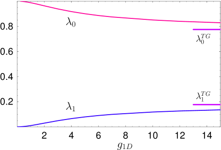
Figure 1: The occupancies $\lambda_{0}$ and $\lambda_{1}$ for a harmonically confined two-boson system in function of $g_{1D}$, their TG limits are marked by horizontal lines.

The state is non-entangled ($\lambda_{0}=1$) only if the bosons do not interact. The weakly entangled ”condensed” state with only one orbital significantly occupied is realized at very weak interactions, $g_{1D}\lesssim 0.1$. With increasing $g_{1D}$, the entanglement grows, which shows up in the increase of $\lambda_{1}$ at the cost of $\lambda_{0}$. The occupancies monotonically approach their TG limits $\lambda_{0}^{TG}\approx 0.7745$ and $\lambda_{1}^{TG}\approx 0.1765$.

Entanglement properties in the case of multi-well potentials are markedly different. Using the optimized RR method, we calculated the natural orbital occupancies of ground states in double-well potential $V_{2{\rm well}}({x})={2\over 27a}(1-ax^{2})^{2}$ and triple-well potential $V_{3{\rm well}}(x)={1\over 2}x^{2}-ax^{4}+{a^{2}\over 2}x^{6}$. The potentials have minima of the same depth and the maxima of the same height, controlled by the parameter $a$. The results for $a=0.025$ are plotted in Figs. 2 and 3, where the upper left presents the shapes of the potentials, and the lower left, the two largest occupancies $\lambda_{0}$ and $\lambda_{1}$ in function of $g_{1D}$. For $g_{1D}=0$, the ground state is non-entangled, as $\lambda_{0}=1$. With increasing interactions, $\lambda_{0}$ decreases and $\lambda_{1}$ grows, monotonically approaching the TG limit of non-entangled ”fragmented” state, $\lambda_{0}^{TG}=\lambda_{1}^{TG}=0.5$. The critical value $g_{1D}^{cr}$, above which $\lambda_{0}\approx\lambda_{1}$, is much larger for the triple-well potential than for the double-well one. The dependence of the two-boson density on $g_{1D}$ for the double-well potential is shown on the right of Fig. 2.

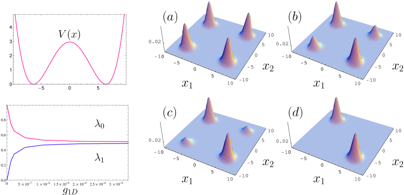
Figure 2: Double-well potential (upper left), the occupancies $\lambda_{0}$ and $\lambda_{1}$ in function of $g_{1D}$ (lower left) and two-boson densities (right) for (a) $g_{1D}=0$, (b) $g_{1D}=2.5\cdot 10^{-8}$, (c) $g_{1D}=5\cdot 10^{-8}$, (d) $g_{1D}=10^{-6}$

For noninteracting bosons, the probability of both being in different wells is the same as being in the same well. With increasing $g_{1D}$, the probability of finding the bosons in the same well quickly decreases and above $g_{1D}^{cr}$ the state is almost fragmented. In the triple-well case (right of Fig. 3) the particles live in the middle well, only above $g_{1D}^{cr}$ the probability of finding a particle in an external well becomes considerable. In the TG limit of non-entangled “fragmented” state, one particle is localized in the middle and the other in one of external wells.

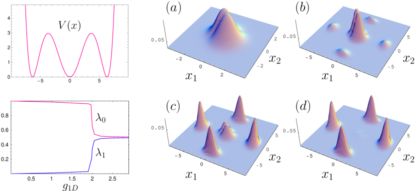
Figure 3: Same as Fig.2 but for the triple-well potential. The two-boson densities (right) for (a) $g_{1D}=1$, (b) $g_{1D}=1.97$, (c) $g_{1D}=1.985$, (d) $g_{1D}=2.05$

4 Conclusion

The optimized CI method proves very effective in determining the spectrum and the natural orbitals of the two-particle confined systems.

References

- [1] Kinoshita, T., Wenger, T., Weiss, D. S.: Science 305, 1125 (2004).
- [2] Girardeau, M.: J.Math.Phys. 1, 516 (1960)
- [3] Helgaker, T., Jørgensen P., Olsen J.: Molecular Electronic- Structure Theory (Wiley, Chichester, 2000).
- [4] Okopińska, A.: Phys.Rev. D36, 1273 (1987)
- [5] Kościk, P., Okopińska, A.: J. Phys. A: Math. Theor. 40, 10851 (2007)
- [6] Busch, T., et al.: Found. Phys. 28, 549 (1998)