Next-to-leading order matrix elements
and truncated showers

Abstract

An algorithm is presented that combines the ME+PS approach to merge sequences of tree-level matrix elements into inclusive event samples [1] with the POWHEG method, which combines exact next-to-leading order matrix elements with parton showers [2]. The quality of the approach and its implementation in Sherpa [3] are exemplified by results for $e^{+}e^{-}$ annihilation into hadrons at LEP, for Drell-Yan lepton-pair production at the Tevatron and for Higgs-boson and $W^{+}W^{-}$-production at LHC energies.

1 Introduction

Facing the huge progress at the LHC, with first data taken, and first results already published, it is crucial to have reliable tools at hand for the full simulation of Standard Model signal and background processes as well as for the simulation of signals for new physics. This task is universally handled by Monte-Carlo event generators like Sherpa [3].

One of the key features of such advanced Monte-Carlo programs is the possibility to consistently combine higher-order tree-level matrix element events with subsequent parton showers (ME+PS) [1]. This feature has proved invaluable in various recent analyses of data from previous experiments, which are sensitive to large-multiplicity final states. Despite being a tremendous improvement over pure leading-order theory, ME+PS merging still suffers from one major drawback of all tree-level calculations, which is their instability with respect to scale variations. This deficiency ultimately necessitates the implementation of NLO virtual corrections in Monte-Carlo programs. Two universally applicable methods were suggested in the past, which can perform this task, and whereof one is the so-called POWHEG algorithm [2]. This technique has been reformulated in [4], such that it can be applied in an automated manner.

Having implementations of both, ME+PS merging and the POWHEG method at our disposal, the question naturally arises, whether the two approaches can be combined into an even more powerful one, joining their respective strengths and eliminating their weaknesses. A first step into this direction was taken independently in [5] and in [6]. Here we will summarise the essence of the algorithms presented ibidem and exemplify the quality of related Monte-Carlo predictions.

2 The MENLOPS approach

A formalism allowing to describe both, the ME+PS and the POWHEG method on the same footing was introduced in [4]. To compare, and, ultimately, to combine both methods, only the expressions for the differential cross section describing the first emission off a given core process must be worked out; this is where the combination takes place.

In a simplified form, the expectation value of an observable in the POWHEG method can be described by the following master formula (for details see [2, 4])

$$\langle O\rangle^{\rm POW}=\sum_{i}\int{\rm d}\Phi_{B}\,\bar{\rm B}_{i}(\Phi_{B})\Bigg{[}\;\underbrace{\bar{\Delta}_{i}(t_{0})\,O(\Phi_{B})}_{\text{no emission}}+\underbrace{\sum_{j}\int_{t_{0}}{\rm d}\Phi_{R|B}\,\frac{{\rm R}_{j}(\Phi_{R})}{{\rm B}_{i}(\Phi_{B})}\;\bar{\Delta}_{i}(t)\,O(\Phi_{R})\;}_{\text{resolved emission}}\Bigg{]}\;,$$ (1)

where $\bar{\rm B}_{i}(\Phi_{B})$ is the NLO-weighted differential cross section for the Born phase-space configuration $\Phi_{B}$ and $\bar{\Delta}_{i}(t)=\exp\left\{\,-\sum_{j}\int_{t}{\rm d}\Phi_{R|B}\,\rm R_{j}/B_{i}\,\right\}$ is the so-called POWHEG-Sudakov form factor. The indices $i$ and $j$ label parton configurations, see [4]. The parameter $t$ is the ordering variable of the underlying parton-shower model and $t_{0}$ is the respective cutoff. Hence, $t$ is one of the variables used to parametrise the radiative phase space $\Phi_{R|B}$.

In a similar manner, a simplified master formula for the expectation value of $O$ in the ME+PS approach can be derived. It reads (for details see [5, 6])

$$\begin{split}&\langle O\rangle^{\rm ME+PS}=\sum_{i}\int{\rm d}\Phi_{B}\,{\rm B}_{i}(\Phi_{B})\Bigg{[}\;\underbrace{\Delta_{i}(t_{0})\,O(\Phi_{B})}_{\text{no emission}}+\sum_{j}\int_{t_{0}}{\rm d}\Phi_{R|B}\\ &\qquad\times\Big{(}\underbrace{\Theta(Q_{\rm cut}-Q)\,\frac{8\pi\alpha_{s}}{t}\,\mathcal{K}_{R_{j}|B_{i}}\,\frac{\mathcal{L}_{R_{j}}}{\mathcal{L}_{B_{i}}}}_{\text{PS domain}}+\underbrace{\Theta(Q-Q_{\rm cut})\,\frac{{\rm R}_{j}(\Phi_{R})}{{\rm B}_{i}(\Phi_{B})}}_{\text{ME domain}}\Big{)}\,\Delta_{i}(t)\,O(\Phi_{R})\;\Bigg{]}\;.\end{split}$$ (2)

The terms labelled “ME domain” and “PS domain” describe the probability of additional QCD radiation according to the real-radiation matrix elements and their corresponding parton-shower approximations, respectively. In this context, $\mathcal{K}_{R_{j}|B_{i}}$ are the parton-shower evolution kernels and $\mathcal{L}_{R_{j}/B_{i}}$ are the parton luminosities of the real-emission and the underlying Born configurations. In contrast to $\bar{\Delta}_{i}(t)$ in Eq. (1), $\Delta_{i}(t)$ is the uncorrected Sudakov form factor of the parton-shower model.

Combining the ME+PS method with POWHEG essentially amounts to combining the two above equations into a new master formula for the MENLOPS approach. This expression reads

$$\begin{split}\langle O\rangle^{\rm MENLOPS}=&\sum_{i}\int{\rm d}\Phi_{B}\,\bar{\rm B}_{i}(\Phi_{B})\Bigg{[}\;\underbrace{\bar{\Delta}_{i}(t_{0})\,O(\Phi_{B})}_{\text{no emission}}+\sum_{j}\int_{t_{0}}{\rm d}\Phi_{R|B}\,\frac{{\rm R}_{j}(\Phi_{R})}{{\rm B}_{i}(\Phi_{B})}\\ &\qquad\times\Big{(}\underbrace{\Theta(Q_{\rm cut}-Q)\,\bar{\Delta}_{i}(t)}_{\text{PS domain}}+\underbrace{\Theta(Q-Q_{\rm cut})\,\Delta_{i}(t)}_{\text{ME domain}}\Big{)}\,O(\Phi_{R})\;\Bigg{]}\;.\end{split}$$ (3)

In order to restore the POWHEG master formula, the “ME domain” term would have to be multiplied by the ratio of Sudakov form factors $\bar{\Delta}_{i}(t)/\Delta_{i}(t)$ only. Expanding this ratio to first order reveals that the above formula automatically yields next-to-leading order accurate predictions for any infrared and collinear safe observable $O$.

3 Results

In the following we present selected results obtained with an implementation of the MENLOPS algorithm in the Sherpa event generator. In particular we aim at detailing the improved description of data collected in various collider experiments.

We focus first on electron-positron annihilation into hadrons at LEP energies ($\sqrt{s}=$91.25 GeV). Virtual matrix elements were supplied by BlackHat [7]. Figure 1 displays distributions of selected angular correlations in 4-jet production, that have been important for tests of perturbative QCD. The good fit to those data proves that correlations amongst the final-state partons are correctly implemented by the higher-order matrix elements in the MENLOPS method.

Similar findings apply in the analysis of the Drell-Yan process at Tevatron energies ($\sqrt{s}=$1.96 TeV). Figure 2 shows the transverse momentum distribution of the reconstructed $Z$-boson and the multiplicity distribution of accompanying jets, constructed using the DØ improved legacy cone algorithm with a cone radius of $R=0.5$, $p_{\perp,j}>20$ GeV and $|\eta_{j}|<2.5$. The agreement of the MENLOPS result with the respective data is outstanding.

We finally present some predictions for the production of Higgs-bosons through gluon-gluon fusion and for the production of $W^{+}[\to\!e^{+}\nu_{e}]\;W^{-}[\to\!\mu^{-}\bar{\nu}_{\mu}]$ at nominal LHC energies ($\sqrt{s}=$14 TeV). Virtual matrix elements for these analyses have been taken from [11] and [12], respectively. Results are shown in Figs. 3 and 4. We observe very small uncertainties related to the intrinsic parameters of the MENLOPS approach. A detailed discussion is found in [6].

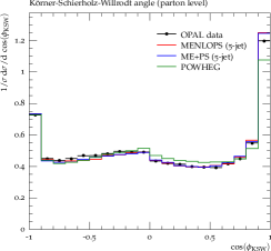
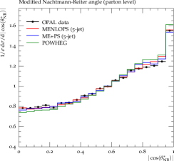
Figure 1: The Körner-Schierholz-Willrodt (KSW) angle (left) and the modified Nachtmann-Reiter (NR) angle (right) in four-jet events defined using the Durham algorithm with $y_{\mathrm{cut}}=0.008$. Results at the parton level are compared to data from the OPAL experiment [8].

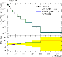
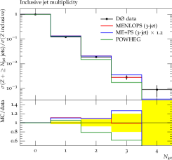
Figure 2: Left: The transverse momentum of the reconstructed $Z$ boson in Drell-Yan events at the Tevatron ($\sqrt{s}=1.96$ TeV). Results obtained with the MENLOPS approach are compared to data from the DØ experiment [9]. Right: Inclusive jet multiplicity in Drell-Yan events. Monte-Carlo predictions are compared to data from [10].

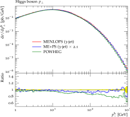
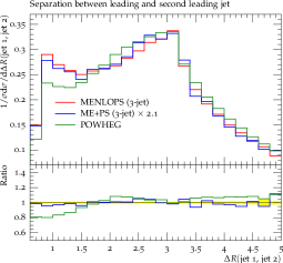
Figure 3: Left: The transverse momentum of the reconstructed Higgs boson in the gluon fusion process at nominal LHC energies (14 TeV). Right: Separation in $\eta$-$\phi$ space of the first and second hardest jet in Higgs-boson production via gluon fusion at nominal LHC energies.

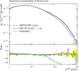
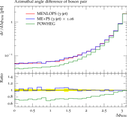
Figure 4: Left: The transverse momentum of the reconstructed $W^{+}W^{-}$ system in $W^{+}[\to\!e^{+}\nu_{e}]\;W^{-}[\to\!\mu^{-}\bar{\nu}_{\mu}]$ events at nominal LHC energies (14 TeV). Right: Separation in $\eta$-$\phi$ space of the first and second hardest jet in $W^{+}W^{-}$ production at nominal LHC energies.

References

- [1] S. Höche, F. Krauss, S. Schumann and F. Siegert, JHEP 0905 (2009) 053 [arXiv:0903.1219 [hep-ph]].
-
[2]
P. Nason,
JHEP 0411 (2004) 040
[hep-ph/0409146];
S. Frixione, P. Nason and C. Oleari, JHEP 0711 (2007) 070 [arXiv:0709.2092 [hep-ph]]. -
[3]
T. Gleisberg, et al. JHEP 0402 (2004) 056
[hep-ph/0311263];
T. Gleisberg, et al. JHEP 0902 (2009) 007 [arXiv:0811.4622 [hep-ph]]. - [4] S. Höche, F. Krauss, M. Schönherr and F. Siegert, arXiv:1008.5399 [hep-ph].
- [5] K. Hamilton and P. Nason, JHEP 1006 (2010) 039 [arXiv:1004.1764 [hep-ph]].
- [6] S. Höche, F. Krauss, M. Schönherr and F. Siegert, arXiv:1009.1127 [hep-ph].
- [7] C. F. Berger et al., Phys. Rev. Lett. 102 (2009) 222001 [arXiv:0902.2760 [hep-ph]].
- [8] G. Abbiendi et al. [OPAL Collaboration], Eur. Phys. J. C 20 (2001) 601 [hep-ex/0101044].
- [9] V. M. Abazov et al. [DØ Collaboration], arXiv:1006.0618 [hep-ex].
- [10] V. M. Abazov et al. [DØ Collaboration], Phys. Lett. B 658 (2008) 112 [hep-ex/0608052].
-
[11]
S. Dawson,
Nucl. Phys. B 359 (1991) 283;
A. Djouadi, M. Spira and P. M. Zerwas, Phys. Lett. B 264 (1991) 440. -
[12]
L. J. Dixon, Z. Kunszt and A. Signer,
Nucl. Phys. B 531 (1998) 3
[hep-ph/9803250];
J. M. Campbell and R. K. Ellis, Phys. Rev. D 60 (1999) 113006 [hep-ph/9905386].