Conformal geometry of surfaces in the Lagrangian–Grassmannian
and second order PDE

Abstract

Contents

1. 1 Introduction
2. 2 The geometry of second order PDE in the plane
   1. 2.1 Jet spaces and the Lagrange–Grassmann bundle
   2. 2.2 Contact transformations
   3. 2.3 Contact invariants for PDE induced from $CSp(4,\mathbb{R})$-invariants for surfaces
3. 3 Conformal geometry of $LG(2,4)$
   1. 3.1 $LG(2,4)$ and $CSp(4,\mathbb{R})$
   2. 3.2 $LG(2,4)$ as a quadric hypersurface in $\mathbb{R}\mathbb{P}^{4}$
   3. 3.3 The invariant conformal structure
   4. 3.4 Elliptic, parabolic, and hyperbolic surfaces
   5. 3.5 Spheres in $LG(2,4)$
   6. 3.6 The Maurer–Cartan form
   7. 3.7 Moving frames for surfaces in $LG(2,4)$
4. 4 Moving frames for hyperbolic surfaces
   1. 4.1 1-adaptation
   2. 4.2 2-adaptation: central sphere congruence
   3. 4.3 Monge–Ampère invariants
   4. 4.4 3-adaptation: cone congruences and the conjugate manifold
5. 5 Hyperbolic surfaces singly-ruled by null geodesics
   1. 5.1 Normalization, invariants, and integrability
   2. 5.2 Geometric interpretation of invariants
   3. 5.3 2-parabolic CSI surfaces and other examples
6. 6 Hyperbolic 2-generic surfaces
   1. 6.1 Normalization, invariants and integrability
   2. 6.2 The conjugate manifold
   3. 6.3 Contact spheres and Dupin cyclides
   4. 6.4 2-generic CSI surfaces and other examples
7. 7 Conclusions
8. A Parametric description of moving frames
   1. A.1 Null parametrization and differential syzygies
   2. A.2 1-adaptation
   3. A.3 Monge–Ampère invariants
   4. A.4 2-adaptation
   5. A.5 3-adaptation for singly-ruled surfaces
   6. A.6 3-adaptation for generic surfaces

1 Introduction

In this article we have two goals in mind: (i) investigate the local differential geometry of hyperbolic (timelike) surfaces in the real Lagrangian–Grassmannian $LG(2,4)$ modulo the conformal symplectic group $CSp(4,\mathbb{R})$, and (ii) investigate the local contact geometry of (in general, highly non-linear) scalar hyperbolic PDE in the plane. Let us describe each in turn and clarify their connection to each other.

Recall that $LG(2,4)$ is the set of isotropic 2-planes with respect to a given symplectic form $\eta$ on $\mathbb{R}^{4}$. As a manifold, $LG(2,4)$ is 3-dimensional and admits a transitive action by the symplectic group $Sp(4,\mathbb{R})$. For our purposes, $\eta$ will be only defined up to scale, hence we use instead $CSp(4,\mathbb{R})$. Our basic question then is: Given two (embedded) surfaces $M,\tilde{M}$ of $LG(2,4)$, does there exist an element $g\in CSp(4,\mathbb{R})$ such that $\tilde{M}=g\cdot M$? We will address this question in the small and seek differential invariants which determine if a neighbourhood of a point in $M$ is equivalent to a neighbourhood of a point in $\tilde{M}$. Most of our study will assume $M,\tilde{M}$ come equipped with parametrizations $i:U\rightarrow M$, $\tilde{i}:U\rightarrow\tilde{M}$ so that equivalence means $\tilde{i}=g\cdot i$ on $U$. Ultimately however, we will be interested in the unparametrized equivalence problem, whereby $i:U\rightarrow M$ and $\tilde{i}:\tilde{U}\rightarrow\tilde{M}$ are equivalent if there is $g\in CSp(4,\mathbb{R})$ and a diffeomorphism $\varphi:U\rightarrow\tilde{U}$ such that $\tilde{i}\circ\varphi=g\cdot i$ on $U$. While the general study of submanifolds in homogeneous spaces is classical [Jen77], our study of surfaces in $LG(2,4)$ modulo $CSp(4,\mathbb{R})$ has not appeared in the literature.

A feature of $LG(2,4)$ absent in higher dimensional Lagrangian–Grassmannians is that $LG(2,4)$ is endowed with a canonical (up to sign) $CSp(4,\mathbb{R})$-invariant Lorentzian conformal structure $[\mu]$, or equivalently a unique $CSp(4,\mathbb{R})$-invariant cone field $\mathcal{C}$. This is a manifestation of the well-known isomorphism $Sp(4,\mathbb{R})\cong Spin(2,3)$, where $Spin(2,3)$ is a double-cover of $SO^{+}(2,3)$, i.e. the identity connected component of $SO(2,3)$. At a deeper level, this comes from the graph isomorphism of the (complex) $\textsf{B}_{2}$ and $\textsf{C}_{2}$ Dynkin diagrams, or corresponding (real) Satake diagrams. With respect to $[\mu]$, $LG(2,4)$ is conformally flat and is diffeomorphic to the indefinite Möbius space $S^{1,2}$.

The study of the Möbius space (conformal sphere) $S^{n}$ of definite signature has a long history. We highlight only the work of Akivis & Goldberg [AG96] which contains an extensive bibliography of the literature on conformal geometry and which was a source of inspiration for our work here. Using moving frames, Akivis & Goldberg carry out a unified study of submanifolds in conformal spaces. However, their study of the indefinite signature case (Section 3.3 in [AG96]) is very brief – e.g. the timelike case occupies only half of p.104 in [AG96]. Four-dimensional conformal structures in all signatures are studied, but it seems that the three-dimensional indefinite case $S^{1,2}\cong LG(2,4)$ was not substantially addressed in their work and has not appeared anywhere in the literature. Thus, one of our goals is to fill in this gap. It should be noted that hypersurface theory in $S^{n}$ for $n\geq 4$ is significantly different than for $S^{3}$. For $n\geq 4$, conformal rigidity of a generic hypersurface is determined by the first fundamental form and trace-free second fundamental form (c.f. Theorem 2.3.1 in [AG96]); for $n=3$, third order invariants come into play [SS80]. In the indefinite case, a similar phenomenon occurs. We also remark that $LG(2,4)$ can be identified with the Lie quadric $Q^{3}$ in Lie sphere geometry [Cec08], whose elements correspond to oriented spheres and points in $\mathbb{R}^{2}$. However, here as well, no study of surfaces in $Q^{3}$ has appeared in the literature.

In spirit, our study is similar to the classical theory of surfaces in Euclidean space $\mathbb{R}^{3}$ modulo the Euclidean group $E(3)$ consisting of rotations, translations and reflections. The mean and Gaussian curvatures feature prominently in this theory. We derive here analogous local invariants for hyperbolic surfaces in $LG(2,4)$ modulo $CSp(4,\mathbb{R})$. Unlike the Euclidean case, any hyperbolic surface is locally conformally flat (see Lemma A.1), so has no intrinsic geometry. Thus, our question is an extrinsic one solely concerned with their embedding into the ambient space $LG(2,4)$.

Our motivation for this study comes from the contact geometry of a scalar second order PDE in the plane (hereafter, simply referred to as a PDE). A PDE $F=0$ can be realized geometrically as a (7-dimensional) hypersurface in the second jet-space $J^{2}=J^{2}(\mathbb{R}^{2},\mathbb{R})$. This ambient jet space is equipped with a canonical contact system $C$ and the geometric theory of such PDE is concerned with the study of such hypersurfaces modulo contact transformations, i.e. those diffeomorphisms preserving $C$. One has the well-known contact-invariant classification into equations of elliptic, parabolic, and hyperbolic type [Gar67]. Less known is the more refined subclassification of hyperbolic PDE into those of Monge–Ampère (MA), Goursat, and generic types (also called class 6-6, 6-7, and 7-7), based on properties of the so-called Monge subsystems [GK93]. All MA PDE are of the form $a(z_{xx}z_{yy}-(z_{xy})^{2})+bz_{xx}+cz_{xy}+dz_{yy}+e=0$ (the coefficients are functions of $x,y,z,z_{x},z_{y}$) and have been well-studied, while relatively little progress has been made on the latter classes, which consist of non-linear equations. For a recent study of generic hyperbolic PDE, see [The08], [The10]. We also highlight the fact that (nonlinear) hyperbolic PDE of the type mentioned above arise as hydrodynamic reductions of certain integrable PDE in three independent variables [Smi09]. We give an equivalent definition of these three hyperbolic classes in terms of the 2nd order $CSp(4,\mathbb{R})$-invariant classification of hyperbolic surfaces in $LG(2,4)$, c.f. Table 2. Roughly, this is possible because:

1. Every fibre $J^{2}|_{\xi}$, for $\xi\in J^{1}$, of the projection map $\pi^{2}_{1}:J^{2}\rightarrow J^{1}$ is diffeomorphic to $LG(2,4)$.

2. The intersection of a hypersurface $F=0$ with each fibre $J^{2}|_{\xi}$ is a two-dimensional surface; the hyperbolicity condition is a first-order condition on this surface.

3. Regarding $C$ as a rank 4 distribution on $J^{1}$ endowed with a (conformal) symplectic form $\eta$, any contact transformation of $J^{2}$ fixing $\xi\in J^{1}$ acts on the fibre $J^{2}|_{\xi}=LG(C_{\xi},[\eta])$ by an element of $CSp(C_{\xi},[\eta])$.

Ours is a fibrewise study of $\pi^{2}_{1}:J^{2}\rightarrow J^{1}$ and $CSp(4,\mathbb{R})$-invariants of surfaces in $LG(2,4)$ yield contact invariants for a PDE. This fibrewise study adds nothing new for MA equations, but new contact invariants are obtained for Goursat and generic equations. Our work here is principally a contribution to the study of fully non-linear hyperbolic PDE.

Added impetus for this work comes from the recent study of curves in general Lagrangian–Grassmannians [Zel05], [ZL07], integrable PDE in three independent variables (hypersurfaces in $LG(3,6)$) [FHK07], integrable $GL(2,\mathbb{R})$ geometry [Smi09], symplectic MA equations in four independent variables (hypersurfaces in $LG(4,8)$) [DF10], and higher-dimensional MA equations [AABMP10]. While the $LG$ realization of the fibres of $\pi^{2}_{1}:J^{2}\rightarrow J^{1}$ dates back at least to work of Yamaguchi [Yam82], we feel this viewpoint is not well-known and has not been sufficiently explored.

Let us give an overview of the contents of our paper. In Section 2, we review the construction of the second jet space $J^{2}$ via the Lagrange–Grassmann bundle. We prove in Theorem 2.7 that $CSp(4,\mathbb{R})$-invariants yield contact invariants for PDE. This is easily seen to hold for $J^{2}(\mathbb{R}^{n},\mathbb{R})$, so more generally: submanifold theory in $LG(n,2n)$ modulo $CSp(2n,\mathbb{R})$ has implications for the contact-invariant study of (systems of) scalar PDE in $n$ independent variables. In Section 3, we delve into the geometry of $LG(2,4)$, taking full advantage of the aforementioned special isomorphism $Sp(4,\mathbb{R})\cong Spin(2,3)$. We describe $LG(2,4)$ as a quadric hypersurface $\mathcal{Q}\subset\mathbb{R}\mathbb{P}^{4}$, and its canonical $CSp(4,\mathbb{R})$-invariant conformal structure and cone field $\mathcal{C}$. To any $[z]\in\mathbb{P}V$ there corresponds a basic surface $\mathcal{S}_{[z]}=\mathbb{P}(z^{\perp})\cap\mathcal{Q}$ which we call a “sphere” of indefinite, definite, or degenerate type (locally, a hyperboloid of one sheet, two sheets, or a cone respectively).

In Section 4, we use Cartan’s method of moving frames to extract invariants of hyperbolic surfaces $M\subset LG(2,4)$. At second order, we recall the conformal Gauss map via the central sphere congruence. Three cases arise: surfaces doubly-ruled or singly-ruled by null geodesics, or generic surfaces. A doubly-ruled hyperbolic surface is shown to be (an open subset of) an indefinite sphere. In local coordinates, spheres take the same form as a MA equation. We recover the well-known theorem on contact-invariance of the hyperbolic MA PDE class via the simple argument:

1. A Monge–Ampère PDE intersects any fibre of $\pi^{2}_{1}:J^{2}\rightarrow J^{1}$ as an indefinite sphere.

2. A contact transformation of $J^{2}$ maps indefinite spheres in any fibre to indefinite spheres in any other fibre.

If $M$ is given a null parametrization, explicit parametrizations of moving frames are given in Appendix A, leading in particular to two relative invariants $I_{1},I_{2}$ which we call Monge–Ampère invariants because of their connection to corresponding contact invariants for hyperbolic PDE. In the PDE setting, the MA invariants were first calculated by Vranceanu [Vra40] for equations of the form $z_{xx}=f(x,y,z,z_{x},z_{y},z_{xy},z_{yy})$. Much later, Juráš [Jur97] calculated these invariants for general $F(x,y,z,z_{x},z_{y},z_{xx},z_{xy},z_{yy})=0$. A third calculation appeared in [The08] which simplified the expression of these invariants. However, all three calculations were significantly involved and did not appeal to the inherent geometry of surfaces in $LG(2,4)$. Our computation here of $I_{1},I_{2}$ based on 2-adapted moving frames is conceptually simple and geometrically motivated: their vanishing characterizes indefinite spheres.

In Sections 5 & 6, we study the geometry of singly-ruled and generic surfaces. For such surfaces $M$, pairs of third order objects called cone congruences can be geometrically associated to $M$. The construction of 3-adapted moving frames leads to the key notion of the conjugate manifold $M^{\prime}$, whose dimension $\dim(M^{\prime})$ is an invariant. If $M^{\prime}$ is also a surface, both $M$, $M^{\prime}$ are envelopes for the central sphere congruence of $M$. For a PDE, a corresponding fibrewise construction leads to the notion of its conjugate PDE. No such notion exists for MA equations since fibrewise these are second order objects (spheres), while the conjugate manifold is a third order construction. In the generic (2-elliptic) case, curvature lines exist which lead to the Lorentzian analogues of contact spheres, canal surfaces, and Dupin cyclides. As a preview, our classification of hyperbolic surfaces / PDE is given in Figure 1. Examples which we will discuss in this paper are given in Figure 2. (See Definition 2.10 for the notion of a CSI PDE.)

Figure 1: Hyperbolic surfaces up to $CSp(4,\mathbb{R})$-equivalence; also, hyperbolic PDE up to contact-equivalence

$$\begin{array}[]{|c|c|c|}\hline\cr\mbox{Hyperbolic PDE}&\mbox{Fibrewise classification as a surface $M\subset LG(2,4)$}&\mbox{CSI?}\\ \hline\cr\hline\cr\begin{array}[]{c}a(z_{xx}z_{yy}-(z_{xy})^{2})+bz_{xx}+cz_{xy}+dz_{yy}+e=0\\ (a,b,c,d,e\mbox{ functions of }x,y,z,z_{x},z_{y})\end{array}&\mbox{indefinite sphere}&\checkmark\\ \hline\cr F(z_{xy},z_{yy})=0&\mbox{indefinite sphere or singly-ruled},\,\dim(M^{\prime})\leq 1&\times\\ \hline\cr z_{xy}=\frac{1}{2}(z_{yy})^{2}&\mbox{singly-ruled},\,\dim(M^{\prime})=0&\checkmark\\ \hline\cr z_{xy}=\exp(z_{yy})&\mbox{singly-ruled},\,\dim(M^{\prime})=1,\,\delta_{1}=+1&\checkmark\\ \hline\cr z_{xy}=\ln(z_{yy})&\mbox{singly-ruled},\,\dim(M^{\prime})=1,\,\delta_{1}=-1&\checkmark\\ \hline\cr F(z_{xx},z_{yy})=0&\mbox{indefinite sphere or 2-elliptic}&\times\\ \hline\cr z_{xx}=\exp(z_{yy})&\mbox{2-elliptic},\,\dim(M^{\prime})=2&\checkmark\\ \hline\cr z_{xx}=\frac{1}{3}(z_{yy})^{3}&\mbox{2-elliptic},\,\dim(M^{\prime})=2&\checkmark\\ \hline\cr z_{xx}z_{yy}=-1&\mbox{2-elliptic, Dupin cyclide},\,\dim(M^{\prime})=2&\checkmark\\ \hline\cr 3z_{xx}(z_{yy})^{3}+1=0&\mbox{2-elliptic},\,\dim(M^{\prime})=0&\checkmark\\ \hline\cr\displaystyle\frac{(3z_{xx}-6z_{xy}z_{yy}+2(z_{yy})^{3})^{2}}{(2z_{xy}-(z_{yy})^{2})^{3}}=c&\left\{\begin{array}[]{l}\mbox{2-elliptic if }c>4,\\ \mbox{2-hyperbolic if }c<0,\\ \mbox{2-hyperbolic if }c=0\\ \quad\mbox{ and }z_{xy}>\frac{1}{2}(z_{yy})^{2}\end{array};\,\right.\dim(M^{\prime})=0&\checkmark\\ &\mbox{(For $0<c\leq 4$, the PDE is not hyperbolic.)}&\\ \hline\cr\end{array}$$

Figure 2: Examples of hyperbolic PDE

The last two entries in Table 2 form the complete list (up to contact equivalence) of maximally symmetric hyperbolic PDE of generic type [The08], each having 9-dimensional contact symmetry algebra. In the case of the latter family, this 9-dimensional Lie algebra is independent of the parameter $c$ and has been shown to be isomorphic to a parabolic subalgebra of the non-compact real form of the 14-dimensional exceptional simple Lie algebra $\mathfrak{g}_{2}$ [The10]. We should also note that while all examples in Figure 2 are of the form $F(z_{xx},z_{xy},z_{yy})=0$, our classification applies equally well to those PDE which have $x,y,z,z_{x},z_{y}$ dependency as well: our classification is fibrewise.

In Section 7, we make some concluding remarks and comment on future directions for research.

2 The geometry of second order PDE in the plane

A scalar second order PDE in the plane can be realized as a hypersurface in $J^{2}=J^{2}(\mathbb{R}^{2},\mathbb{R})$. We review the geometric construction of the jet spaces $J^{k}=J^{k}(\mathbb{R}^{2},\mathbb{R})$ for $k\leq 2$. This section generalizes to more independent variables than two, but we restrict to two for simplicity and since this is our main focus in this paper.

2.1 Jet spaces and the Lagrange–Grassmann bundle

Identify the zeroth order jet space $J^{0}$ with $\mathbb{R}^{3}$, regarded as a trivial bundle with fibre $\mathbb{R}$ over the base $\mathbb{R}^{2}$. Define the first order jet space $J^{1}$ to be the Grassmann bundle $Gr(2,T\mathbb{R}^{3})$, with projection $\pi^{1}_{0}:J^{1}\rightarrow J^{0}$. Any $\xi\in J^{1}$ is a 2-plane in $T_{\bar{\xi}}\mathbb{R}^{3}$, where $\bar{\xi}=\pi^{1}_{0}(\xi)$. There is a canonical linear Pfaffian system $(\mathcal{I},\mathcal{J})$ on $J^{1}$ given by

$$\mathcal{I}|_{\xi}=(\pi^{1}_{0})^{*}(\xi^{\perp}),\qquad\mathcal{J}|_{\xi}=(\pi^{1}_{0})^{*}(T^{*}_{\bar{\xi}}\mathbb{R}^{3}).$$

The canonical system $C$ (also called the contact distribution) on $J^{1}$ is defined by $C_{\xi}=(\pi^{1}_{0})_{*}{}^{-1}(\xi)\subset T_{\xi}J^{1}$.

Let us examine this in local coordinates. Let $\xi_{0}\in J^{1}$, $\bar{\xi}_{0}=\pi^{1}_{0}(\xi_{0})$. Pick local coordinates $(x,y,z)$ on an open set $\bar{U}\subset\mathbb{R}^{3}$ about $\bar{\xi}_{0}$ such that $dx\wedge dy|_{\xi_{0}}\neq 0$. By continuity, $dx\wedge dy|_{\xi}\neq 0$ for all $\xi$ in some neighbourhood $U\subset(\pi^{1}_{0})^{-1}(\bar{U})$ about $\xi_{0}$. Since $\xi$ is 2-dimensional and $dx|_{\xi},dy|_{\xi}$ are linearly independent, then on $U$,

$$dz|_{\xi}=p(\xi)dx|_{\xi}+q(\xi)dy|_{\xi}.$$

This defines local coordinates $p=p(\xi),q=q(\xi)$. Hence, $\xi=span\{D_{x},D_{y}\}\in Gr(2,T_{\bar{\xi}}\mathbb{R}^{3})$, where

$$D_{x}=\left.\frac{\partial}{\partial x}\right|_{\bar{\xi}}+p(\xi)\left.\frac{\partial}{\partial z}\right|_{\bar{\xi}},\qquad D_{y}=\left.\frac{\partial}{\partial y}\right|_{\bar{\xi}}+q(\xi)\left.\frac{\partial}{\partial z}\right|_{\bar{\xi}}.$$

Pulling back $J^{0}$ coordinates to $J^{1}$, $(x,y,z,p,q)$ are local coordinates on $J^{1}$, $\mathcal{I}$ is generated by the contact 1-form $\sigma=dz-pdx-qdy$, and $\mathcal{J}=\{dz,dx,dy\}$ is associated with the independence condition $dx\wedge dy\neq 0$. Finally,

$$C=\{\sigma=0\}=span\left\{\frac{\partial}{\partial x}+p\frac{\partial}{\partial z},\frac{\partial}{\partial y}+q\frac{\partial}{\partial z},\frac{\partial}{\partial p},\frac{\partial}{\partial q}\right\}.$$ (2.1)

The exterior derivative $\eta=d\sigma=dx\wedge dp+dy\wedge dq$ restricts to be a non-degenerate (conformal) symplectic form on the distribution $C$. (Only the conformal class of $\eta$ is relevant since $\sigma$ is only well-defined up to scale.) With respect to the basis given in (2.1), $\eta$ is represented by $\left(\begin{array}[]{cc}0&I_{2}\\ -I_{2}&0\end{array}\right)$, where $I_{2}$ is the $2\times 2$ identity matrix. We define the second jet space $J^{2}$ as the Lagrange–Grassmann bundle $LG(C,[\eta])$ over $J^{1}$, with projection $\pi^{2}_{1}:J^{2}\rightarrow J^{1}$, i.e.

$$J^{2}=\bigcup_{\xi\in J^{1}}J^{2}|_{\xi}:=\bigcup_{\xi\in J^{1}}LG(C_{\xi},[\eta]).$$

Namely, any $\tilde{\xi}\in J^{2}$ is a Lagrangian (i.e. 2-dimensional isotropic) subspace of $(C_{\xi},[\eta])$, where $\xi=\pi^{2}_{1}(\tilde{\xi})$. Since $(C_{\xi},[\eta])$ is isomorphic to $\mathbb{R}^{4}$ with its canonical (conformal) symplectic form, it is clear that the fibres of $\pi^{2}_{1}$ are all diffeomorphic to $LG(2,4)$, which has dimension 3. This identification is of course not canonical since there is no preferred basepoint. The canonical system on $J^{2}$ is given by $\tilde{C}_{\tilde{\xi}}=(\pi^{2}_{1})_{*}{}^{-1}(\tilde{\xi})\subset T_{\tilde{\xi}}J^{2}$.

Given $\tilde{\xi}_{0}\in J^{2}$, pick adapted local coordinates $(x,y,z,p,q)$ (as above) on a neighbourhood $U$ of $\xi_{0}=\pi^{2}_{1}(\tilde{\xi}_{0})\in J^{1}$ with $dx\wedge dy|_{\tilde{\xi}_{0}}\neq 0$. Define $\tilde{U}=\{\tilde{\xi}\in(\pi^{2}_{1})^{-1}(U):dx\wedge dy|_{\tilde{\xi}}\neq 0\}$. For any $\tilde{\xi}\in\tilde{U}$, define $r(\tilde{\xi}),s_{1}(\tilde{\xi}),s_{2}(\tilde{\xi}),t(\tilde{\xi})$ by

$$dp|_{\tilde{\xi}}=r(\tilde{\xi})dx|_{\tilde{\xi}}+s_{1}(\tilde{\xi})dy|_{\tilde{\xi}},\qquad dq|_{\tilde{\xi}}=s_{2}(\tilde{\xi})dx|_{\tilde{\xi}}+t(\tilde{\xi})dy|_{\tilde{\xi}}.$$

Since $\tilde{\xi}$ is Lagrangian, then on $\tilde{\xi}$ we have $0=\eta=d\sigma=dx\wedge dp+dy\wedge dq=(s_{1}-s_{2})dx\wedge dy$ so that $s_{1}=s_{2}$. Letting $s:=s_{1}=s_{2}$, we have $\tilde{\xi}=span\{\tilde{D}_{x},\tilde{D}_{y}\}\in LG(C_{\xi},[\eta])\subset Gr(2,TJ^{1})$, where

$$\tilde{D}_{x}=\left.\frac{\partial}{\partial x}\right|_{\xi}+p(\xi)\left.\frac{\partial}{\partial z}\right|_{\xi}+r(\tilde{\xi})\left.\frac{\partial}{\partial p}\right|_{\xi}+s(\tilde{\xi})\left.\frac{\partial}{\partial q}\right|_{\xi},\qquad\tilde{D}_{y}=\left.\frac{\partial}{\partial y}\right|_{\xi}+q(\xi)\left.\frac{\partial}{\partial z}\right|_{\xi}+s(\tilde{\xi})\left.\frac{\partial}{\partial p}\right|_{\xi}+t(\tilde{\xi})\left.\frac{\partial}{\partial q}\right|_{\xi}.$$ (2.2)

Pulling back the $J^{1}$ coordinates $(x,y,z,p,q)$ to $J^{2}$, we have a local coordinate system $(x,y,z,p,q,r,s,t)$ on $J^{2}$. We call such coordinates standard. The canonical system $\tilde{C}$ is given by $\tilde{C}=\{\sigma=\sigma^{1}=\sigma^{2}=0\}$, where

$$\sigma=dz-pdx-qdy,\qquad\sigma^{1}=dp-rdx-sdy,\qquad\sigma^{2}=dq-sdx-tdy.$$

We see that for sections $\mathbb{R}^{2}\rightarrow J^{2}$, $(x,y)\rightarrow(x,y,z,p,q,r,s,t)$, on which $\sigma=\sigma^{1}=\sigma^{2}=0$, we have

$$p=z_{x},\quad q=z_{y},\quad r=z_{xx},\quad s=z_{xy},\quad t=z_{yy}.$$

2.2 Contact transformations

Definition 2.1.

A (local) contact transformation of $J^{1}$ [or $J^{2}$] is a (local) diffeomorphism preserving the canonical system $C$ [or $\tilde{C}$] under pushforward.

Any contact transformation $\phi$ of $J^{1}$ prolongs to a contact transformation ${\rm pr}(\phi)$ of $J^{2}$, i.e. $\phi_{*}$ acts on $C$, inducing a map of Lagrangian–Grassmannians ${\rm pr}(\phi):J^{2}|_{\xi}\rightarrow J^{2}|_{\xi^{\prime}}$. In particular, ${\rm pr}(\phi)$ preserves fibres of $\pi^{2}_{1}:J^{2}\rightarrow J^{1}$. Conversely, by Backlünd’s theorem [Olv95], if $\tilde{\phi}$ on $J^{2}$ is contact, then $\tilde{\phi}={\rm pr}(\phi)$ for some $\phi$ contact on $J^{1}$.

Example 2.2.

It is well-known that (for scalar-valued maps) there are contact transformations of $J^{1}$ that are not the prolongation of diffeomorphisms of $J^{0}$. An example of this is the Legendre transformation $(\bar{x},\bar{y},\bar{z},\bar{p},\bar{q})=(-p,-q,z-px-qy,x,y)$, which satisfies $\bar{\sigma}=d\bar{z}-\bar{p}d\bar{x}-\bar{q}d\bar{y}=d(z-px-qy)+xdp+ydq=\sigma$.

Since $\phi$ is contact, then $\phi^{*}\sigma=\lambda\sigma$, for some function $\lambda$ on $J^{1}$, which implies for $\eta=d\sigma$ that $\phi^{*}\eta=\phi^{*}d\sigma=d(\phi^{*}\sigma)=d\lambda\wedge\sigma+\lambda\eta$. Restricting to $C=\{\sigma=0\}$, we see that $\eta$ is preserved up to the overall factor of $\lambda$, i.e. $\phi_{*}:(C_{\xi},[\eta])\rightarrow(C_{\xi^{\prime}},[\eta])$ is a conformal symplecticomorphism. If $\xi^{\prime}=\phi(\xi)=\xi$, then $\phi_{*}\in CSp(C_{\xi},[\eta])$ and this acts on $J^{2}|_{\xi}$. Conversely, one may ask if, given $\xi\in J^{1}$, any element of $CSp(C_{\xi},[\eta])$ is realized by a local contact transformation of $J^{2}$. This question has an affirmative answer, but we postpone the proof until Section 3.1. These observations motivate our study of surfaces in $LG(2,4)$ modulo $CSp(4,\mathbb{R})$ (as opposed to a smaller subgroup).

2.3 Contact invariants for PDE induced from $CSp(4,\mathbb{R})$-invariants for surfaces

Consider a second order scalar PDE in the plane $F=0$, regarded as a hypersurface $\Sigma$ in $J^{2}$. We use the usual non-degeneracy assumption that $\Sigma$ is transverse to $\pi^{2}_{1}:J^{2}\rightarrow J^{1}$ and that $\pi^{2}_{1}|_{\Sigma}:\Sigma\rightarrow J^{1}$ is a submersion. Given $\xi\in J^{1}$, consider the fibre $J^{2}|_{\xi}=(\pi^{2}_{1})^{-1}(\xi)=LG(C_{\xi},[\eta])$ and $\Sigma|_{\xi}=\Sigma\cap J^{2}|_{\xi}$, which is a 2-dimensional surface. We now discuss the transfer of differential invariants from the standard $LG(2,4)$ setting to the PDE setting. For now, simply regard $LG(2,4)$ as the set of isotropic 2-planes on the standard $(\mathbb{R}^{4},[\eta])$ with standard basis and $CSp(4,\mathbb{R})$ consists of linear transformations of $\mathbb{R}^{4}$ which preserve $\eta$ up to scale.

Let $U$ be a 2-dimensional connected manifold. Let $J^{n}(U,LG(2,4))$ denote the $n$-th order jet space of maps $s:U\rightarrow LG(2,4)$. The action of $g\in CSp(4,\mathbb{R})$ prolongs to an action $g^{(n)}$ on $J^{n}(U,LG(2,4))$, c.f. [Olv95] or [Sau89].

Definition 2.3.

An $n$-th order differential invariant for $CSp(4,\mathbb{R})$ is a function $\kappa:J^{n}(U,LG(2,4))\rightarrow\mathbb{R}$ such that $\kappa(g^{(n)}\cdot{\bf p})=\kappa({\bf p})$, for any $g\in CSp(4,\mathbb{R})$ and ${\bf p}\in J^{n}(U,LG(2,4))$. For short, we call $\kappa$ a $CSp(4,\mathbb{R})$-invariant.

Example 2.4.

We will endow $LG(2,4)$ with natural coordinates $(r,s,t)$ and the conformal structure $[drdt-ds^{2}]$. Locally, $J^{1}(U,LG(2,4))$ is given by $(u,v,r,s,t,r_{u},r_{v},s_{u},s_{v},t_{u},t_{v})$. The sign of the determinant of

$$\left(\begin{array}[]{cc}r_{u}t_{u}-s_{u}{}^{2}&\frac{1}{2}r_{u}t_{v}+\frac{1}{2}r_{v}t_{u}-s_{u}s_{v}\\ \frac{1}{2}r_{u}t_{v}+\frac{1}{2}r_{v}t_{u}-s_{u}s_{v}&r_{v}t_{v}-s_{v}{}^{2}\end{array}\right)$$

is a first-order $CSp(4,\mathbb{R})$-invariant, distinguishing hyperbolic (timelike), parabolic (null), elliptic (spacelike) surfaces.

Definition 2.5.

Let $(W,[\eta])$ be a 4-dimensional real vector space endowed with a conformal symplectic form. A conformal symplectic (c.s.) basis $\textsf{{\em b}}=\{e_{i}\}_{i=1}^{4}$ is a basis of $W$ such that the matrix $(\eta(e_{i},e_{j}))_{i,j=1}^{4}$ is a multiple of $\left(\begin{array}[]{cccc}0&I_{2}\\ -I_{2}&0\end{array}\right)$. The first two vectors $e_{1},e_{2}$ of b span a Lagrangian subspace, i.e. an element of $LG(W,[\eta])$.

Lemma 2.6.

A $CSp(4,\mathbb{R})$-invariant $\kappa:J^{n}(U,LG(2,4))\rightarrow\mathbb{R}$ induces a $CSp(C_{\xi},[\eta])$-invariant $\kappa_{\xi}:J^{n}(U,J^{2}|_{\xi})\rightarrow\mathbb{R}$.

Proof.

Fix any c.s. basis b of $(C_{\xi},[\eta])$. This defines an isomorphism (conformal symplectomorphism) $\psi_{\textsf{b}}:C_{\xi}\rightarrow\mathbb{R}^{4}$ by mapping b onto the standard basis of $\mathbb{R}^{4}$, hence induces $\tilde{\psi}_{\textsf{b}}:J^{2}|_{\xi}\stackrel{{\scriptstyle\cong}}{{\rightarrow}}LG(2,4)$ and identifies $\widehat{\psi}_{\textsf{b}}:CSp(C_{\xi},[\eta])\stackrel{{\scriptstyle\cong}}{{\rightarrow}}CSp(4,\mathbb{R})$. Note that for $g\in CSp(C_{\xi},[\eta])$ and $g_{\textsf{b}}=\widehat{\psi}_{\textsf{b}}(g)\in CSp(4,\mathbb{R})$, we have:

$$\psi_{g\cdot\textsf{b}}\circ g=\psi_{\textsf{b}},\qquad\psi_{\textsf{b}}\circ g=g_{\textsf{b}}\circ\psi_{\textsf{b}},$$ (2.3)

with similar identities for $\tilde{\psi}_{\textsf{b}}$. Given a $CSp(4,\mathbb{R})$-invariant $\kappa$, define $\kappa_{\xi}:J^{n}(U,J^{2}|_{\xi})\rightarrow\mathbb{R}$ by $\kappa_{\xi}(j^{n}_{x}s):=\kappa(j^{n}_{x}(\tilde{\psi}_{\textsf{b}}\circ s))$, where $s:U\rightarrow J^{2}|_{\xi}$ is a local map and $j^{n}_{x}s$ is the $n$-th jet prolongation of $s$ evaluated at $x\in U$. We claim:

1. $\kappa_{\xi}$ is well-defined: Let $\textsf{b}^{\prime}$ be another c.s. basis, so $\textsf{b}^{\prime}=g\cdot\textsf{b}$ for some $g\in CSp(C_{\xi},[\eta])$. By (2.3), $\kappa(j^{n}_{x}(\tilde{\psi}_{\textsf{b}^{\prime}}\circ s))=\kappa(j^{n}_{x}(\tilde{\psi}_{\textsf{b}}\circ g^{-1}\circ s))=\kappa((g_{\textsf{b}}{}^{-1})^{(n)}\cdot j^{n}_{x}(\tilde{\psi}_{\textsf{b}}\circ s))=\kappa(j^{n}_{x}(\tilde{\psi}_{\textsf{b}}\circ s))$.

2. $\kappa_{\xi}$ is $CSp(C_{\xi},[\eta])$-invariant: Fix $g\in CSp(C_{\xi},[\eta])$. By (2.3), $\kappa_{\xi}(g^{(n)}\cdot j^{n}_{x}s)=\kappa_{\xi}(j^{n}_{x}(g\cdot s))=\kappa(j^{n}_{x}(\tilde{\psi}_{\textsf{b}}\circ(g\cdot s)))=\kappa(j^{n}_{x}(g_{\textsf{b}}\cdot(\tilde{\psi}_{\textsf{b}}\circ s)))=\kappa(g_{\textsf{b}}{}^{(n)}\cdot j^{n}_{x}(\tilde{\psi}_{\textsf{b}}\circ s))=\kappa(j^{n}_{x}(\tilde{\psi}_{\textsf{b}}\circ s))=\kappa_{\xi}(j^{n}_{x}s)$.

∎

The function $\kappa_{\xi}$ accounts for “vertical” derivatives, i.e. derivatives only along the fibre $J^{2}|_{\xi}$. Consider the bundle $\mathbb{J}^{n}:=\dot{\bigcup}_{\xi\in J^{1}}J^{n}(U,J^{2}|_{\xi})$ over $J^{1}$. Given a contact transformation $\tilde{\phi}:J^{2}\rightarrow J^{2}$ and a map $s:U\rightarrow J^{2}|_{\xi}$, we have $\tilde{\phi}\circ s:U\rightarrow J^{2}|_{\phi(\xi)}$, hence we define $\Phi^{(n)}:\mathbb{J}^{n}\rightarrow\mathbb{J}^{n}$ by $\Phi^{(n)}(j^{n}_{x}s):=j^{n}_{x}(\tilde{\phi}\circ s)$. Define $\textsf{K}:\mathbb{J}^{n}\rightarrow\mathbb{R}$ by $\textsf{K}({\bf p})=\kappa_{\xi}({\bf p})$, where ${\bf p}\in J^{n}(U,J^{2}|_{\xi})$. We say that K is contact-invariant if $\textsf{K}\circ\Phi^{(n)}=\textsf{K}$ for any contact transformation $\tilde{\phi}:J^{2}\rightarrow J^{2}$.

Theorem 2.7.

Any $CSp(4,\mathbb{R})$-invariant $\kappa:J^{n}(U,LG(2,4))\rightarrow\mathbb{R}$ induces a contact-invariant function $\textsf{K}:\mathbb{J}^{n}\rightarrow\mathbb{R}$. In particular, for any constant $c\in\mathbb{R}$, $\textsf{K}=c$ defines a contact-invariant class of PDE.

Proof.

To show K is contact-invariant, we show $\kappa_{\phi(\xi)}(\Phi^{(n)}(j^{n}_{x}s))=\kappa_{\xi}(j^{n}_{x}s)$ for any contact $\tilde{\phi}={\rm pr}(\phi):J^{2}\rightarrow J^{2}$ and $s:U\rightarrow J^{2}|_{\xi}$. If $\phi(\xi)=\xi$, then $\tilde{\phi}\in CSp(C_{\xi},[\eta])$, so by $CSp(C_{\xi},[\eta])$-invariance, $\kappa_{\xi}\circ\Phi^{(n)}=\kappa_{\xi}$. If $\phi(\xi)\neq\xi$, choose any c.s. basis $\textsf{b}=\{e_{i}\}_{i=1}^{4}$ of $(C_{\xi},[\eta])$. Since $\phi_{*}$ is a conformal symplectomorphism, then $\textsf{b}^{\prime}=\{e_{i}^{\prime}=\phi_{*}(e_{i})\}_{i=1}^{4}$ is also a c.s. basis. We have $\kappa_{\phi(\xi)}(\Phi^{(n)}(j^{n}_{x}s))=\kappa_{\phi(\xi)}(j^{n}_{x}(\tilde{\phi}\circ s))=\kappa(j^{n}_{x}(\tilde{\psi}_{\textsf{b}^{\prime}}\circ\tilde{\phi}\circ s))=\kappa(j^{n}_{x}(\tilde{\psi}_{\textsf{b}}\circ s))=\kappa_{\xi}(j^{n}_{x}s)$. ∎

Remark 2.8.

Theorem 2.7 clearly generalizes to $J^{2}(\mathbb{R}^{n},\mathbb{R})$: Submanifold theory in $LG(n,2n)$ modulo $CSp(2n,\mathbb{R})$ has implications for the contact-invariant study of systems of scalar PDE in $n$ independent variables.

For any surface $M\subset LG(2,4)$ (as for a PDE) there is no distinguished choice of (local) parametrization $i:U\rightarrow M$ and hence invariants that we seek should be independent of reparametrization. Thus, we are ultimately interested in the unparametrized equivalence problem: Given $i:U\rightarrow M$ and $\tilde{i}:\tilde{U}\rightarrow\tilde{M}$, does there exist a diffeomorphism $\varphi:U\rightarrow\tilde{U}$ and an element $g\in CSp(4,\mathbb{R})$ such that $\tilde{i}\circ\varphi=g\cdot i$ on $U$? We will study this problem in three steps:

1. Apply Cartan’s method of moving frames to find invariants for the parametrized equivalence problem.

2. Give a parametric description of the invariants of the parametrized problem. There is a natural choice of coordinates $(r,s,t)$ on $LG(2,4)$ which correspond to the 2nd derivative coordinates in the PDE setting.

3. Investigate how the above invariants change under reparametrization. Unchanged properties will be invariants for the unparametrized equivalence problem.

Generally, the simplest surfaces to describe are those with constant $CSp(4,\mathbb{R})$-invariants $\kappa$. Surfaces in $LG(2,4)$ which have all constant symplectic ($CSp(4,\mathbb{R})$) invariants (CSI) have a natural geometric meaning:

Proposition 2.9 (Homogeneity theorem, p.42 of [Jen77]).

For any smooth embedding $i:U\rightarrow G/H$, $M=i(U)$ is an open submanifold of a homogeneous submanifold of $G/H$ iff $M$ has no non-constant $G$-invariants.

Definition 2.10.

Let $\Sigma\subset J^{2}$ be a PDE. If for any (well-defined) $CSp(4,\mathbb{R})$-invariant $\kappa$ of surfaces in $LG(2,4)$ the corresponding contact-invariant K is constant on $\Sigma$, then we call $\Sigma$ a constant symplectic invariant (CSI) PDE.

Several examples of hyperbolic CSI PDE are given in Figure 2.

3 Conformal geometry of $LG(2,4)$

In Section 2, our main result was that $CSp(4,\mathbb{R})$-invariants for surfaces in $LG(2,4)$ induce contact-invariants for PDE. With this in mind, we describe the ambient geometry of $LG(2,4)$ with a view to preparing for our later study of hyperbolic surfaces via the method of moving frames.

3.1 $LG(2,4)$ and $CSp(4,\mathbb{R})$

On $\mathbb{R}^{4}$, take the standard basis $\{e_{i}\}_{i=1}^{4}$ with dual basis $\{\eta^{i}\}_{i=1}^{4}$. Let $\eta=2(\eta^{1}\wedge\eta^{3}+\eta^{2}\wedge\eta^{4})$ be the standard symplectic form represented by $J=\left(\begin{array}[]{cc}0&I_{2}\\ -I_{2}&0\end{array}\right)$, so $\eta(x,y)={x}^{\mathsf{T}}Jy$. We define:

$$Sp(4,\mathbb{R}) =\left\{X\in GL(4,\mathbb{R}):{X}^{\mathsf{T}}JX=J\right\}=\left\{\left(\begin{array}[]{cc}A&B\\ C&D\end{array}\right):{A}^{\mathsf{T}}C={C}^{\mathsf{T}}A,\,{B}^{\mathsf{T}}D={D}^{\mathsf{T}}B,\,{A}^{\mathsf{T}}D-{C}^{\mathsf{T}}B=I_{2}\right\},$$

$$\mathfrak{sp}(4,\mathbb{R}) =\left\{X\in Mat_{4\times 4}(\mathbb{R}):{X}^{\mathsf{T}}J+JX=0\right\}=\left\{\left(\begin{array}[]{cc}a&b\\ c&-{a}^{\mathsf{T}}\end{array}\right):b,c\mbox{ symmetric}\right\},$$

which are 10-dimensional. $LG(2,4)$ is the set of $\eta$-isotropic 2-planes in $\mathbb{R}^{4}$. This admits a transitive $Sp(4,\mathbb{R})$-action, hence $LG(2,4)=Sp(4,\mathbb{R})/P$ up to a choice of basepoint $o$. Choosing $o=span\{e_{1},e_{2}\}$, we see $\dim(P)=7$ since

$$P=\left\{\left(\begin{array}[]{cc}A&B\\ 0&({A}^{\mathsf{T}})^{-1}\end{array}\right):A\in GL(2,\mathbb{R}),A^{-1}B\mbox{ symmetric}\right\},\qquad\mathfrak{p}=\left\{\left(\begin{array}[]{cc}a&b\\ 0&-{a}^{\mathsf{T}}\end{array}\right):b\mbox{ symmetric}\right\}.$$

Hence, $\dim(LG(2,4))=3$. The $Sp(4,\mathbb{R})$-action is not effective: the global isotropy subgroup is $K=\{\pm I_{4}\}\cong\mathbb{Z}_{2}$.

In the PDE context (Section 2.1), only the conformal class $[\eta]$ is relevant. This does not affect the definition of $LG(2,4)$ since a 2-plane is $\eta$-isotropic iff it is $(\lambda\eta)$-isotropic. We consider instead the conformal symplectic group

$$CSp(4,\mathbb{R}) =\left\{X\in GL(4,\mathbb{R}):{X}^{\mathsf{T}}JX=\rho J,\mbox{ for some }\rho\in\mathbb{R}^{\times}\right\}\cong Sp(4,\mathbb{R})\rtimes_{\varphi}\mathbb{R}^{\times},$$

where $\mathbb{R}^{\times}$ is embedded into $GL(4,\mathbb{R})$ as $\rho\mapsto{\rm diag}(\rho I_{2},I_{2})$ and note that $\varphi:\mathbb{R}^{\times}\rightarrow Aut(Sp(4,\mathbb{R}))$ by

$$\varphi(\rho)\left(\begin{array}[]{cc}A&B\\ C&D\end{array}\right)=\left(\begin{array}[]{cc}\rho I_{2}&0\\ 0&I_{2}\end{array}\right)\left(\begin{array}[]{cc}A&B\\ C&D\end{array}\right)\left(\begin{array}[]{cc}\rho^{-1}I_{2}&0\\ 0&I_{2}\end{array}\right)=\left(\begin{array}[]{cc}A&\rho B\\ \rho^{-1}C&D\end{array}\right).$$

Since $diag(\sqrt{\rho}{}^{-1}I_{2},\sqrt{\rho}I_{2})\cdot diag(\rho I_{2},I_{2})=\sqrt{\rho}I_{4}$ acts trivially, then $\rho\in\mathbb{R}^{\times}$ and $diag(\sqrt{\rho}I_{2},\sqrt{\rho}{}^{-1}I_{2})\in P$ have the same action on $LG(2,4)$. Most of $\mathbb{R}^{\times}$ is redundant and it suffices to consider $\widehat{Sp}(4,\mathbb{R})=Sp(4,\mathbb{R})\rtimes_{\varphi}\mathbb{Z}_{2}$, where $\mathbb{Z}_{2}$ is generated by $\rho=-1$, i.e. $diag(-I_{2},I_{2})$. The stabilizer in $\widehat{Sp}(4,\mathbb{R})$ of $o$ is $\widehat{P}=P\rtimes\mathbb{Z}_{2}$, and global isotropy is $K$.

Let us describe a collection of charts on general $LG(n,2n)$. For more details, see [PT03]. A Lagrangian decomposition of $(\mathbb{R}^{2n},\eta)$ is a pair $(L_{0},L_{1})$ of transversal Lagrangian subspaces in $LG(n,2n)$, i.e. $\mathbb{R}^{2n}=L_{0}\oplus L_{1}$ and $L_{0}\cap L_{1}=0$. Define $\,\pitchfork\!\!(L_{1})=\{L\in LG(n,2n):L\mbox{ transverse to }L_{1}\}$ and $B_{sym}(L_{0})=\{\mbox{symmetric bilinear forms on }L_{0}\}$. Associated to any Lagrangian decomposition $(L_{0},L_{1})$ is a chart $\psi_{L_{0},L_{1}}=\rho_{L_{0},L_{1}}\circ\phi_{L_{0},L_{1}}:\,\pitchfork\!\!(L_{1})\rightarrow B_{sym}(L_{0})$, where the maps $\phi_{L_{0},L_{1}}:\,\pitchfork\!\!(L_{1})\rightarrow Lin(L_{0},L_{1})$ and $\rho_{L_{0},L_{1}}:L_{1}\rightarrow L_{0}{}^{*}$ are defined by

$$\phi_{L_{0},L_{1}}(L)=T_{L},\qquad\rho_{L_{0},L_{1}}(v)=\eta(\cdot,v)|_{L_{0}}$$ (3.1)

Here, $T_{L}$ is uniquely defined by $L=graph(T_{L})=\{v+T_{L}(v):v\in L_{0}\}$. A priori the image of $\psi_{L_{0},L_{1}}$ is in $B(L_{0})$, but in fact $\psi_{L_{0},L_{1}}$ is a bijection onto $B_{sym}(L_{0})$. Moreover, the collection of charts as $(L_{0},L_{1})$ ranges over all Lagrangian decompositions yields a differentiable atlas for $LG(n,2n)$ [PT03].

Let $L_{0}=o=span\{e_{1},e_{2}\}$ and $L_{1}=span\{e_{3},e_{4}\}$. We describe the chart $\psi=\psi_{L_{0},L_{1}}$ on $LG(2,4)$. From above,

$$L=span\{\tilde{e}_{1}=e_{1}+re_{3}+se_{4},\,\,\tilde{e}_{2}=e_{2}+se_{3}+te_{4}\}\in\,\pitchfork\!\!(L_{1})\quad\stackrel{{\scriptstyle\psi}}{{\longmapsto}}\quad\left(\begin{array}[]{cc}r&s\\ s&t\end{array}\right).$$ (3.4)

The right side of (3.4) is the matrix for: (i) $T_{L}\in Lin(L_{0},L_{1})$ in the bases $\{e_{1},e_{2}\},\{e_{3},e_{4}\}$, or (ii) $\psi(L)\in B_{sym}(L_{0})$ in the basis $\{e_{1},e_{2}\}$. Equivalently, exponentiate $X=\left(\begin{array}[]{cc}r&s\\ s&t\end{array}\right)$ on $\mathfrak{sp}(4,\mathbb{R})/\mathfrak{p}$ to obtain $\left(\begin{array}[]{cc}I_{2}&0\\ X&I_{2}\end{array}\right)/P$ on $LG(2,4)=Sp(4,\mathbb{R})/P$, and the first two columns yield the left side of (3.4). From (2.1) and (2.2), the fibrewise identification

$$e_{1}=\partial_{x}+p\partial_{z},\quad e_{2}=\partial_{y}+q\partial_{z},\quad e_{3}=\partial_{p},\quad e_{4}=\partial_{q}$$ (3.5)

implies that these $(r,s,t)$ coordinates in $LG(2,4)$ correspond to the natural $(r,s,t)$ coordinates in the $J^{2}$ setting. Hereafter, whenever we write $(r,s,t)$, we mean such coordinates in one setting or the other.

Now let us see the $\widehat{Sp}(4,\mathbb{R})$-action in the chart $\psi$. The element $\rho=-1\in\mathbb{Z}_{2}$ acts as $(r,s,t)\mapsto(-r,-s,-t)$. For elements in $Sp(4,\mathbb{R})$ sufficiently close to the identity,

$$\left(\begin{array}[]{cc}A&B\\ C&D\end{array}\right)\cdot\left(\begin{array}[]{cc}I&0\\ X&I\end{array}\right)/P=\left(\begin{array}[]{cc}A+BX&B\\ C+DX&D\end{array}\right)/P=\left(\begin{array}[]{cc}I&0\\ \tilde{X}&I\end{array}\right)/P,$$ (3.14)

so we have the Möbius-like transformation $\tilde{X}=(C+DX)(A+BX)^{-1}$. Table 1 displays the infinitesimal generators.

$\begin{array}[]{|c|c||c|c||c|c|}\hline\cr\vrule\lx@intercol\hfil\mbox{Rotations}\hfil\lx@intercol\vrule\lx@intercol\vrule\lx@intercol&\vrule\lx@intercol\hfil\mbox{Inversions}\hfil\lx@intercol\vrule\lx@intercol\vrule\lx@intercol&\vrule\lx@intercol\hfil\mbox{Translations}\hfil\lx@intercol\vrule\lx@intercol\\ \hline\cr\hline\cr a_{11}&-2r\partial_{r}-s\partial_{s}&b_{1}&-r^{2}\partial_{r}-rs\partial_{s}-s^{2}\partial_{t}&c_{1}&\partial_{r}\\ a_{12}&-r\partial_{s}-2s\partial_{t}&b_{2}&-s^{2}\partial_{r}-st\partial_{s}-t^{2}\partial_{t}&c_{2}&\partial_{t}\\ a_{21}&-2s\partial_{r}-t\partial_{s}&b_{3}&-2rs\partial_{r}-(s^{2}+rt)\partial_{s}-2st\partial_{t}&c_{3}&\partial_{s}\\ a_{22}&-s\partial_{s}-2t\partial_{t}&&&&\\ \hline\cr\end{array}$

Table 1: Infinitesimal generators for $\mathfrak{sp}(4,\mathbb{R})$-action on $LG(2,4)$

We now address the claim at the end of Section 2.2.

Proposition 3.1.

Given $\xi\in J^{1}$, any element of $CSp(C_{\xi},[\eta])$ is realized by a local contact transformation of $J^{2}$.

Proof.

Fix $\xi\in J^{1}$. Choose coordinates $(x,y,z,p,q)$ on $J^{1}$ as in Section 2.1 such that $\xi=(x,y,z,p,q)=(0,0,0,0,0)$. As in (3.5), we identify the $(r,s,t)$ coordinates in the $LG(2,4)$ and $J^{2}|_{\xi}$ settings. Next, we realize the vector fields in Table 1 as the $(r,s,t)$ components of a prolongation ${\bf X}^{(2)}$ of a contact symmetry ${\bf X}$.

$$\begin{array}[]{|c|c|c|}\hline\cr{\bf X}&{\bf X}^{(2)}&(r,s,t)\mbox{ components of }{\bf X}^{(2)}\\ \hline\cr\hline\cr\frac{1}{2}x^{2}\partial_{z}&\frac{1}{2}x^{2}\partial_{z}+x\partial_{p}+\partial_{r}&\partial_{r}\\ xy\partial_{z}&xy\partial_{z}+y\partial_{p}+x\partial_{q}+\partial_{s}&\partial_{s}\\ \frac{1}{2}y^{2}\partial_{z}&\frac{1}{2}y^{2}\partial_{z}+y\partial_{q}+\partial_{t}&\partial_{t}\\ \hline\cr x\partial_{x}&x\partial_{x}-p\partial_{p}-2r\partial_{r}-s\partial_{s}&-2r\partial_{r}-s\partial_{s}\\ y\partial_{x}&y\partial_{x}-p\partial_{q}-r\partial_{s}-2s\partial_{t}&-r\partial_{s}-2s\partial_{t}\\ x\partial_{y}&x\partial_{y}-q\partial_{p}-2s\partial_{r}-t\partial_{s}&-2s\partial_{r}-t\partial_{s}\\ y\partial_{y}&y\partial_{y}-q\partial_{q}-s\partial_{s}-2t\partial_{t}&-s\partial_{s}-2t\partial_{t}\\ \hline\cr p\partial_{x}+\frac{p^{2}}{2}\partial_{z}&p\partial_{x}+\frac{p^{2}}{2}\partial_{z}-r^{2}\partial_{r}-rs\partial_{s}-s^{2}\partial_{t}&-r^{2}\partial_{r}-rs\partial_{s}-s^{2}\partial_{t}\\ q\partial_{x}+p\partial_{y}+pq\partial_{z}&q\partial_{x}+p\partial_{y}+pq\partial_{z}-2rs\partial_{r}-(s^{2}+rt)\partial_{s}-2st\partial_{t}&-2rs\partial_{r}-(s^{2}+rt)\partial_{s}-2st\partial_{t}\\ q\partial_{y}+\frac{q^{2}}{2}\partial_{z}&q\partial_{y}+\frac{q^{2}}{2}\partial_{z}-s^{2}\partial_{r}-st\partial_{s}-t^{2}\partial_{t}&-s^{2}\partial_{r}-st\partial_{s}-t^{2}\partial_{t}\\ \hline\cr\end{array}$$

Since the components of all ${\bf X}^{(1)}:=(\pi^{2}_{1})_{*}{\bf X}^{(2)}$ above are homogeneous in $(x,y,z,p,q)$, then restricted to $\xi=(0,0,0,0,0)$, these are vertical vector fields for the projection $\pi^{2}_{1}$, i.e. they preserve $J^{2}|_{\xi}=LG(C_{\xi},[\eta])$. Thus, any infinitesimal generator of the $CSp(C_{\xi},[\eta])$-action on $J^{2}|_{\xi}$ is realizable by an infinitesimal contact transformation. But $Sp(4,\mathbb{R})\cong Sp(C_{\xi},\eta)$ is connected so this is true in terms of regular (finite) transformations. Lastly, if $\rho\in\mathbb{R}^{\times}$, the contact transformation $(x,y,z,p,q)\mapsto(\rho x,\rho y,\rho z,p,q)$ preserves $J^{2}|_{\xi}$ and induces $\eta\mapsto\rho\eta$. ∎

Because of Proposition 3.1, we can easily recognize various transformations of $LG(2,4)$ from their corresponding jet transformations. For example, in the jet space setting we know the scalings $(x,y,z)\rightarrow(\lambda_{1}x,\lambda_{2}y,\mu z)$ induces $(r,s,t)\rightarrow(\frac{\mu}{\lambda_{1}{}^{2}}r,\frac{\mu}{\lambda_{1}\lambda_{2}}s,\frac{\mu}{\lambda_{2}{}^{2}}t)$. Hence, the latter is also a transformation of $LG(2,4)$.

3.2 $LG(2,4)$ as a quadric hypersurface in $\mathbb{R}\mathbb{P}^{4}$

By the Plücker embedding, the full Grassmannian $Gr(2,4)$ embeds as the decomposable elements in $\mathbb{P}(\textstyle{\bigwedge}^{2}\mathbb{R}^{4})$. The induced $\widehat{Sp}(4,\mathbb{R})$-action on $\textstyle{\bigwedge}^{2}\mathbb{R}^{4}$ preserves $V:=\textstyle{\bigwedge}^{2}_{0}\mathbb{R}^{4}=\{z\in\textstyle{\bigwedge}^{2}\mathbb{R}^{4}:\eta(z)=0\}$, which is a 5-dimensional irreducible subspace. The restriction of the Plücker embedding to $LG(2,4)$ has image the quadric hypersurface $\mathcal{Q}=\left\{[z]\in\mathbb{P}V:\langle z,z\rangle=0\right\}$, where $\langle z_{1},z_{2}\rangle=3(\eta\wedge\eta)(z_{1}\wedge z_{2})$ is a non-degenerate symmetric bilinear form. Note that $3(\eta\wedge\eta)(e_{1}\wedge e_{2}\wedge e_{3}\wedge e_{4})=-24(\eta^{1}\wedge\eta^{2}\wedge\eta^{3}\wedge\eta^{4})(e_{1},e_{2},e_{3},e_{4})=-\det(\eta^{i}(e_{j}))=-1$. On $V$, take the basis

$$\mathcal{B}:\quad\begin{array}[]{l}e_{1}\wedge e_{2},\\ e_{3}\wedge e_{2},\\ e_{1}\wedge e_{3}-e_{2}\wedge e_{4},\\ e_{1}\wedge e_{4},\\ e_{3}\wedge e_{4}\end{array}\quad\Rightarrow\quad\langle\cdot,\cdot\rangle_{\mathcal{B}}=\left(\begin{array}[]{ccccc}0&0&0&0&-1\\ 0&0&0&1&0\\ 0&0&-2&0&0\\ 0&1&0&0&0\\ -1&0&0&0&0\end{array}\right),$$ (3.25)

so $\langle\cdot,\cdot\rangle$ has signature $(2,3)=(++---)$. Since $LG(2,4)$ is $\widehat{Sp}(4,\mathbb{R})$-invariant, so are $\mathcal{Q}$ and $\langle\cdot,\cdot\rangle$. Fixing the basis $\mathcal{B}$, there is a homomorphism $\Phi:\widehat{Sp}(4,\mathbb{R})\rightarrow O(2,3)$. The induced Lie algebra homomorphism $\phi=\Phi_{*}:\mathfrak{sp}(4,\mathbb{R})\rightarrow\mathfrak{so}(2,3)$ given by

$$\phi\left(\begin{array}[]{cccc}a_{11}&a_{12}&b_{1}&b_{3}\\ a_{21}&a_{22}&b_{3}&b_{2}\\ c_{1}&c_{3}&-a_{11}&-a_{21}\\ c_{3}&c_{2}&-a_{12}&-a_{22}\end{array}\right)=\left(\begin{array}[]{ccccc}a_{11}+a_{22}&b_{1}&2b_{3}&b_{2}&0\\ c_{1}&a_{22}-a_{11}&-2a_{21}&0&b_{2}\\ c_{3}&-a_{12}&0&-a_{21}&-b_{3}\\ c_{2}&0&-2a_{12}&a_{11}-a_{22}&b_{1}\\ 0&c_{2}&-2c_{3}&c_{1}&-(a_{11}+a_{22})\end{array}\right)$$ (3.35)

is an isomorphism. Since $Sp(4,\mathbb{R})$ is connected and $O(2,3)$ has four connected components, then $\Phi$ yields a 2-to-1 covering map $Sp(4,\mathbb{R})\rightarrow SO^{+}(2,3)$, so $Sp(4,\mathbb{R})\cong Spin(2,3)$. The element $\rho=-1\in\mathbb{Z}_{2}$ acts on $\mathcal{B}$ as the matrix $diag(1,-1,-1,-1,1)$ which has determinant $-1$. Hence, $\Phi:\widehat{Sp}(4,\mathbb{R})\rightarrow O^{+}(2,3)$ is surjective with kernel $K=\{\pm I_{4}\}$. The effective symmetry group of $\mathcal{Q}$ is $O^{+}(2,3)$ with stabilizer $P^{+}=\Phi(P)$ at $[e_{1}\wedge e_{2}]$.

Remark 3.2.

As groups, $O(2,3)/SO^{+}(2,3)\cong\mathbb{Z}_{2}\times\mathbb{Z}_{2}$. Let $V_{+},V_{-}$ be the maximal positive and negative definite subspaces of $V$. Here, $O^{+}(2,3)\subset O(2,3)$ preserves the orientation of $V_{-}$, e.g. $-I\in O^{-}(2,3)$.

We can write the condition $\langle z,z\rangle=0$ defining $\mathcal{Q}$ in coordinates as $|x|^{2}-|y|^{2}:=x_{1}{}^{2}+x_{2}{}^{2}-y_{1}{}^{2}-y_{2}{}^{2}-y_{3}{}^{2}=0$, where $[z]=[(x,y)]\in\mathcal{Q}$ and we may assume $x\in S^{1}$, $y\in S^{2}$. Since $[(x,y)]=[(-x,-y)]$, then $LG(2,4)\cong(S^{1}\times S^{2})/\mathbb{Z}_{2}$.

With respect to the chart $\psi$ in Section 3.1, the Lagrangian subspace $L=span\{\tilde{e}_{1},\tilde{e}_{2}\}$ in (3.4) satisfies

$$\tilde{e}_{1}\wedge\tilde{e}_{2}=e_{1}\wedge e_{2}+re_{3}\wedge e_{2}+s(e_{1}\wedge e_{3}+e_{4}\wedge e_{2})+te_{1}\wedge e_{4}+(rt-s^{2})e_{3}\wedge e_{4},$$

so with respect to $\mathcal{B}$, $L=[1,r,s,t,rt-s^{2}]\in\mathcal{Q}$. Thus, $\psi:[1,r,s,t,rt-s^{2}]\in\mathcal{Q}\longmapsto(r,s,t)\in\mathbb{R}^{3}$. Points of $LG(2,4)$ not covered by $\psi^{-1}$ are $\{[0,a,b,c,d]:ac-b^{2}=0\}$, which is precisely the degenerate sphere $\mathcal{S}_{[{\bf Z}]}$ (see Section 3.5), where ${\bf Z}=(0,0,0,0,1)$, and can be regarded as the “sphere at infinity”.

Consider a second coordinate chart $\psi^{\prime}$ centered at ${\bf Z}$, i.e. $span\{e_{3},e_{4}\}$ by taking $(e_{1}^{\prime},e_{2}^{\prime},e_{3}^{\prime},e_{4}^{\prime})=(e_{3},e_{4},-e_{1},-e_{2})$ and constructing similar coordinates $[1,r^{\prime},s^{\prime},t^{\prime},r^{\prime}t^{\prime}-(s^{\prime})^{2}]_{\mathcal{B}^{\prime}}=$ as above with respect to the new basis $\mathcal{B}^{\prime}$. Relating $\mathcal{B}^{\prime}$ to $\mathcal{B}$, we see $[1,r^{\prime},s^{\prime},t^{\prime},r^{\prime}t^{\prime}-(s^{\prime})^{2}]_{\mathcal{B}^{\prime}}=[rt-s^{2},-t,s,-r,1]_{\mathcal{B}^{\prime}}$. Thus, the coordinate change formula $\psi^{\prime}\circ\psi^{-1}$ is

$$r^{\prime}=\frac{-t}{rt-s^{2}},\qquad s^{\prime}=\frac{s}{rt-s^{2}},\qquad t^{\prime}=\frac{-r}{rt-s^{2}}.$$ (3.36)

In fact, at least three coordinate charts are needed to cover $LG(2,4)$. The set of points in $\mathcal{Q}$ not covered by $\psi^{-1}$ or $(\psi^{\prime})^{-1}$ is $\mathcal{Q}\cap\{[0,a,b,c,0]:ac-b^{2}=0\}$. In the PDE setting, the Legendre transformation (see Example 2.2) prolongs to give (3.36) on the $J^{2}$ coordinates $(r,s,t)$ .

3.3 The invariant conformal structure

There is a distinguished (up to sign) Lorentzian conformal structure $[\mu]$, equivalently a cone field $\mathcal{C}=\{\mu=0\}$, on $LG(2,4)$, which we describe here in three ways. A fourth description is given in Section 3.6.

A conformal structure $[\mu]$ is an equivalence class of metrics: $\mu\sim\mu^{\prime}$ iff $\mu^{\prime}=\lambda^{2}\mu$, where $\lambda$ is nonvanishing. For conformal structures, all $\widehat{Sp}(4,\mathbb{R})$-invariant ones on $LG(2,4)$ correspond to $Ad(\widehat{P})$-invariant ones on $\mathfrak{sp}(4,\mathbb{R})/\mathfrak{p}=\left\{\left(\begin{array}[]{cc}0&0\\ c&0\end{array}\right):c\mbox{ symmetric}\right\}/\mathfrak{p}.$ The element $\rho=-1$ in the $\mathbb{Z}_{2}$ factor of $\widehat{P}$ acts as $c\mapsto-c$. Via the adjoint action,

$$\left(\begin{array}[]{cc}A&B\\ 0&({A}^{\mathsf{T}})^{-1}\end{array}\right)\cdot\left(\begin{array}[]{cc}0&0\\ c&0\end{array}\right)/\mathfrak{p}=\left(\begin{array}[]{cc}0&0\\ ({A}^{\mathsf{T}})^{-1}cA^{-1}&0\end{array}\right)/\mathfrak{p}.$$ (3.43)

Note $\det(c)$ transforms as $\det(c)\mapsto\det(A)^{-2}\det(c)$. The conformal class of its polarization is $Ad(\widehat{P})$-invariant and corresponds to an $\widehat{Sp}(4,\mathbb{R})$-invariant conformal structure $[\mu]$ on $LG(2,4)$. In fact, $[\pm\mu]$ are the only two such structures. Thus, $LG(2,4)$ is endowed with a canonical $CSp(4,\mathbb{R})$-invariant cone field $\mathcal{C}=\{\mu=0\}$.

For a second description, let $\widehat{\mathcal{Q}}=\{z\in V:\langle z,z\rangle=0\}=cone(\mathcal{Q})$. For any $[z]\in\mathcal{Q}$ and $\rho\in\mathbb{R}^{\times}$, the affine tangent space $\widehat{T}_{[z]}\mathcal{Q}$ is the tangent space to $\widehat{\mathcal{Q}}$ at any $\rho z$, translated to the origin, i.e.

$$\widehat{T}_{[z]}\mathcal{Q}=T_{\rho z}\mathcal{\widehat{Q}}=T_{z}\mathcal{\widehat{Q}}=\{w:\langle z,w\rangle=0\}=z^{\perp},\quad\dim(z^{\perp})=4.$$

The canonical surjection $\pi:V\rightarrow\mathbb{P}V$ restricts to $\pi:\mathcal{\widehat{Q}}\rightarrow\mathcal{Q}$ and induces vector space isomorphisms $(\pi_{*})_{\rho z}:z^{\perp}/\ell_{z}\rightarrow T_{[z]}\mathcal{Q}$, where $\ell_{z}=span\{z\}$. These satisfy $(\pi_{*})_{\rho z}(\rho w)=(\pi_{*})_{z}(w)$, $\forall w\in z^{\perp}$. The form induced by $\langle\cdot,\cdot\rangle$ on $z^{\perp}/\ell_{z}$ is non-degenerate and has signature $(1,2)$. This transfers to $T_{[z]}\mathcal{Q}$ via $(\pi_{*})_{z}$ or $(\pi_{*})_{\rho z}$ and these differ by a factor of $\rho^{2}$. This conformal class on $T_{[z]}\mathcal{Q}$ induces a conformal structure on all of $\mathcal{Q}$. It is $\widehat{Sp}(4,\mathbb{R})$-invariant because so is $\langle\cdot,\cdot\rangle$.

Remark 3.3.

Although $(\pi_{*})_{\rho z}$ depends on $\rho\in\mathbb{R}^{\times}$, there is a well-defined mapping of subspaces since $(\pi_{*})_{\rho z}=\frac{1}{\rho}(\pi_{*})_{z}$, e.g. if $M\subset\mathcal{Q}$ is a submanifold, then $T_{[z]}M$ is identified with a subspace of $z^{\perp}/\ell_{z}$. Alternatively, there is the canonical isomorphism $z^{\perp}/\ell_{z}\stackrel{{\scriptstyle\cong}}{{\rightarrow}}\ell_{z}\otimes T_{[z]}\mathcal{Q}$, $[w]\mapsto\rho z\otimes(\pi_{*})_{\rho z}(w)=z\otimes(\pi_{*})_{z}(w)$, or equivalently, $\ell_{z}^{*}\otimes(z^{\perp}/\ell_{z})\cong T_{[z]}\mathcal{Q}$.

We have a third description in terms of the local coordinates $(r,s,t)$ in the chart $\psi$. Taking $c=\left(\begin{array}[]{cc}r&s\\ s&t\end{array}\right)$ in (3.43), the invariant conformal structure $[\mu]$ has representative $\mu=dr\odot dt-ds\odot ds=drdt-ds^{2}$. Each vector field $Z$ in Table 1 preserves $[\mu]$ under Lie derivation, i.e. $\mathcal{L}_{Z}\mu=\lambda(Z)\mu$ for some scalar function $\lambda(Z)$. Given a tangent vector $v=v_{1}\frac{\partial}{\partial r}+v_{2}\frac{\partial}{\partial s}+v_{3}\frac{\partial}{\partial t}$, $\mu(v,v)=v_{1}v_{3}-v_{2}{}^{2}$ and this is positive / zero / negative iff $v$ lies inside [on, outside] the null cone. This is well-defined on the conformal class $[\mu]$.

3.4 Elliptic, parabolic, and hyperbolic surfaces

Definition 3.4.

Let $M\subset LG(2,4)$ be a surface. We say $M$ is:

1. elliptic (spacelike) if for any $x\in M$, $T_{x}M\cap\mathcal{C}_{x}$ is a single point; equivalently, $N_{x}M$ is timelike.

2. parabolic (null) if for any $x\in M$, $T_{x}M\cap\mathcal{C}_{x}$ consists of a single line; equivalently, $N_{x}M$ is null.

3. hyperbolic (timelike) if for any $x\in M$, $T_{x}M\cap\mathcal{C}_{x}$ consists of two distinct lines; equivalently, $N_{x}M$ is spacelike.

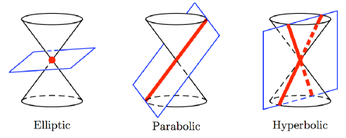
Figure 3: Intersection types

In the chart $\psi$, suppose $M$ has equation $F(r,s,t)=0$. On $M$, $0=dF=F_{r}dr+F_{s}ds+F_{t}dt$. Assuming $(F_{r},F_{s},F_{t})\neq 0$ on $M$, then $T_{x}M$ for any $x\in M$ is spanned by the (linearly dependent) vectors $F_{r}\partial_{s}-F_{s}\partial_{r}$, $F_{t}\partial_{r}-F_{r}\partial_{t}$, $F_{t}\partial_{s}-F_{s}\partial_{t}$. The $\mu$-orthogonal complement of $T_{x}M$ yields the normal space $N_{x}M$ spanned by $n=F_{t}\frac{\partial}{\partial r}-\frac{1}{2}F_{s}\frac{\partial}{\partial s}+F_{r}\frac{\partial}{\partial t}$ and we have $\mu(n,n)=F_{r}F_{t}-\frac{1}{4}F_{s}{}^{2}$, whose sign is well-defined on $[\mu]$. Hence, $M$ is elliptic / parabolic / hyperbolic iff at each point of $M$, $F_{r}F_{t}-\frac{1}{4}F_{s}{}^{2}$ is positive / zero / negative.

Example 3.5.

Let $c\neq 0$ be a constant. The surface $rt=c$ is elliptic if $c>0$ and hyperbolic if $c<0$. Using the rescaling $(r,s,t)\rightarrow(\lambda r,\lambda s,\lambda t)$ which is a $CSp(4,\mathbb{R})$ transformation, all are equivalent to $rt=1$ or $rt=-1$.

The canonical cone field $\mathcal{C}$ on $LG(2,4)$ transfers to each fibre $J^{2}|_{\xi}$ in the PDE setting. Alternatively, the sign of $\mu(n,n)$ is a discrete $CSp(4,\mathbb{R})$-invariant on $M$, which by Theorem 2.7 yields a contact-invariant for PDE. Surprisingly, even the following definition has not appeared in the literature.

Definition 3.6.

$\Sigma=\{F=0\}\subset J^{2}$ is elliptic / parabolic / hyperbolic at $\tilde{\xi}\in J^{2}$ if for $\xi=\pi^{2}_{1}(\tilde{\xi})$, $T_{\tilde{\xi}}(\Sigma|_{\xi})$ intersects the canonical cone ${\cal C}_{\tilde{\xi}}\subset T_{\tilde{\xi}}(J^{2}|_{\xi})$ in one point / along one line / along two distinct lines. Equivalently, the normal line to $T_{\tilde{\xi}}(\Sigma|_{\xi})\subset T_{\tilde{\xi}}(J^{2}|_{\xi})$ lies inside / on / outside ${\cal C}_{\tilde{\xi}}$.

Thus, from the $LG$ perspective, “elliptic / parabolic / hyperbolic” is really a first order consequence of the existence of the cone field $\mathcal{C}$, which itself is a manifestation of the special isomorphism $Sp(4,\mathbb{R})\cong Spin(2,3)$. In standard $J^{2}$ coordinates $(x,y,z,p,q,r,s,t)$, the sign of $F_{r}F_{t}-\frac{1}{4}F_{s}{}^{2}$ evaluated pointwise on $\Sigma$ determines the PDE type. We recover the usual invariant distinguishing elliptic, parabolic, hyperbolic PDE [Gar67].

3.5 Spheres in $LG(2,4)$

Using $\langle\cdot,\cdot\rangle$, there is a bijective (polar) correspondence between points and hyperplanes in $\mathbb{P}V$.

Definition 3.7.

For any $[z]\in\mathbb{P}V$, we refer to $\mathcal{S}_{[z]}=\mathbb{P}(z^{\perp})\cap\mathcal{Q}$ as a sphere.

Remark 3.8.

We caution the reader that spheres as we have defined above are topologically different from the usual spheres in Euclidean geometry. Rather, a sphere above is the intersection of a hyperplane with $\mathcal{Q}$. This terminology is borrowed from classical conformal geometry in definite signature.

Orthogonality characterizes incidence with $\mathcal{S}_{[z]}$: if $[w]\in\mathcal{Q}$, then $[w]\in\mathcal{S}_{[z]}$ iff $\langle w,z\rangle=0$. Hence, spheres are given by linear equations. Let $\mathcal{H}_{+}=\{[z]\in\mathbb{P}V:\langle z,z\rangle>0\}$ and $\mathcal{H}_{-}=\{[z]\in\mathbb{P}V:\langle z,z\rangle<0\}$. Then $\mathbb{P}V=\mathcal{H}_{+}\dot{\cup}\,\mathcal{H}_{-}\dot{\cup}\,\mathcal{Q}$. The spheres determined by elements in $\mathcal{H}_{+},\mathcal{H}_{-},\mathcal{Q}$ are referred to as definite, indefinite, degenerate respectively. Note that any $[z]\in\mathcal{Q}$ plays a dual role as: (i) a point in $\mathcal{Q}$, and (ii) a sphere in $\mathcal{Q}$ with vertex (singularity) at $[z]$.

Lemma 3.9.

1. $Sp(4,\mathbb{R})$ acts transitively on each of $\mathcal{H}_{+},\mathcal{H}_{-},\mathcal{Q}$.

2. Let $\langle z,z\rangle<0$. The stabilizer in $Sp(4,\mathbb{R})$ of $[z]$ acts transitively on $\mathcal{S}_{[z]}$.

Proof.

Exercise for the reader. ∎

Using Lemma 3.9, and by examining points in $\mathcal{H}_{+},\mathcal{H}_{-},\mathcal{Q}$, the corresponding spheres are topologically $\mathbb{R}\mathbb{P}^{2}$, $(S^{1}\times S^{1})/\mathbb{Z}_{2}$, and a pinched torus respectively. However, this will not play an essential role in the sequel. More relevant for us is the local picture. Let us describe general spheres in the chart $\psi$. With respect to the basis $\mathcal{B}$ in Section 3.2, fix $z=(z_{0},z_{1},z_{2},z_{3},z_{4})\in V$ and note $\langle z,z\rangle=2(z_{1}z_{3}-z_{2}{}^{2}-z_{4}z_{0})$. Then

$$\psi(\mathcal{S}_{[z]}) =\{(r,s,t):-z_{4}+rz_{3}-2sz_{2}+tz_{1}-z_{0}(rt-s^{2})=0\}.$$ (3.44)

If $z_{0}=0$, then $\psi(\mathcal{S}_{[z]})$ is a plane, while if $z_{0}\neq 0$, then $\psi(\mathcal{S}_{[z]})=\left\{(r,s,t):\left(r-\frac{z_{1}}{z_{0}}\right)\left(t-\frac{z_{3}}{z_{0}}\right)-\left(s-\frac{z_{2}}{z_{0}}\right)^{2}=\frac{\langle z,z\rangle}{2z_{0}{}^{2}}\right\}$ is a hyperboloid of 2-sheets, a hyperboloid of 1-sheet, or a cone iff $\langle z,z\rangle$ is positive, negative, or zero, respectively.

Proposition 3.10.

Let $[z]\in\mathcal{H}_{-}$. The indefinite sphere $\mathcal{S}_{[z]}$ is doubly-ruled by null geodesics.

Proof.

For any $[w]\in\mathcal{S}_{[z]}$, $\widehat{T}_{[w]}\mathcal{S}_{[z]}=w^{\perp}\cap z^{\perp}$ has signature $(+-0)$ since $\langle z,z\rangle<0$ and $\langle\cdot,\cdot\rangle$ has signature $(2,3)$. Hence, we can choose a null basis $\{u_{1},u_{2},w\}$ of $\widehat{T}_{[w]}\mathcal{S}_{[z]}$. Let $u$ be either $u_{1}$ or $u_{2}$. Then $u$ correponds to a null direction in the tangent space $T_{[w]}\mathcal{S}_{[z]}$. Also, $\langle u,u\rangle=\langle u,w\rangle=\langle u,z\rangle=0$. For any $a,b\in\mathbb{R}$ (not both zero), $\langle au+bw,au+bw\rangle=0$, so $[au+bw]\in\mathcal{Q}$ and $\langle au+bw,z\rangle=0$, so $[au+bw]$ is a null projective line contained in $\mathcal{S}_{[z]}$, which is a null line in the chart $\psi$. Since the conformal structure $[\mu]$ is flat, null lines are null geodesics. ∎

For our later study of hyperbolic surfaces in $LG(2,4)$, consider the basis

$$\mathcal{B}_{H}:\quad\begin{array}[]{l}e_{1}\wedge e_{2},\\ e_{3}\wedge e_{2},\\ e_{1}\wedge e_{4},\\ e_{1}\wedge e_{3}-e_{2}\wedge e_{4},\\ e_{3}\wedge e_{4}\end{array}\quad\Rightarrow\quad\langle\cdot,\cdot\rangle_{\mathcal{B}_{H}}=\left(\begin{array}[]{ccccc}0&0&0&0&-1\\ 0&0&1&0&0\\ 0&1&0&0&0\\ 0&0&0&-2&0\\ -1&0&0&0&0\end{array}\right),$$ (3.55)

which is $\mathcal{B}$ (3.25) with third and fourth basis vectors interchanged. Any basis $\textsf{v}=(\textsf{v}_{0},...,\textsf{v}_{4})$ of $V$ with scalar products $\langle\textsf{v}_{i},\textsf{v}_{j}\rangle$ given by the matrix in (3.55) will be called a hyperbolic frame. Any such frame has a natural geometric interpretation as a 5-tuple of spheres: $([\textsf{v}_{0}],[\textsf{v}_{1}],[\textsf{v}_{2}],[\textsf{v}_{4}])$ forms a null diamond inscribed in the indefinite sphere $\mathcal{S}_{[\textsf{v}_{3}]}$. The picture given in Figure 4 is a sample configuration, but should not be misleading: e.g. one or more of the points $[\textsf{v}_{i}]$, $i=1,2,3,4$, may lie at on the sphere at infinity. (If $[\textsf{v}_{3}]$ is, then the hyperboloid degenerates to a plane.)

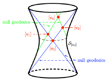
Figure 4: Geometric interpretation of a hyperbolic frame

Let $\mathcal{P}_{x}\in LG(2,4)$ correspond to $[x]\in\mathcal{Q}\subset\mathbb{P}V$ under the Plücker map. The following is obvious:

Lemma 3.11.

Let $[x],[y]\in\mathcal{Q}$. Then $\langle x,y\rangle\neq 0$ iff $\mathbb{R}^{4}=\mathcal{P}_{x}\oplus\mathcal{P}_{y}$ is a Lagrangian decomposition. Thus, if $[x]\neq[y]$ and $\langle x,y\rangle=0$, then $\dim(\mathcal{P}_{x}\cap\mathcal{P}_{y})=1$.

Thus, given a basis v of $V$ as above, we can interpret it in the symplectic setting. Corresponding to v, we have

• we have a pair of Lagrangian decompositions $\mathbb{R}^{4}=\mathcal{P}_{[\textsf{v}_{0}]}\oplus\mathcal{P}_{[\textsf{v}_{4}]}$ and $\mathbb{R}^{4}=\mathcal{P}_{[\textsf{v}_{1}]}\oplus\mathcal{P}_{[\textsf{v}_{3}]}$.

• $\mathcal{P}_{[\textsf{v}_{0}]}=(\mathcal{P}_{[\textsf{v}_{0}]}\cap\mathcal{P}_{[\textsf{v}_{1}]})\oplus(\mathcal{P}_{[\textsf{v}_{0}]}\cap\mathcal{P}_{[\textsf{v}_{3}]})$ and $\mathcal{P}_{[\textsf{v}_{4}]}=(\mathcal{P}_{[\textsf{v}_{4}]}\cap\mathcal{P}_{[\textsf{v}_{3}]})\oplus(\mathcal{P}_{[\textsf{v}_{4}]}\cap\mathcal{P}_{[\textsf{v}_{1}]})$.

Finally, inversion with respect to an indefinite or definite sphere $\mathcal{S}_{[z]}$ is defined in a natural manner: Let $[w]\in\mathcal{Q}$. Its inversion $[\tilde{w}]$ with respect to $\mathcal{S}_{[z]}$ is $\tilde{w}=w-\frac{2\langle w,z\rangle}{\langle z,z\rangle}z$. If $[\tilde{w}]=[w]$, we must have $\tilde{w}=w$ and $\langle w,z\rangle=0$, i.e. $[w]\in\mathcal{S}_{[z]}$. Inversion with respect to a degenerate sphere is undefined.

3.6 The Maurer–Cartan form

Recall the effective symmetry group of $\mathcal{Q}=LG(2,4)$ is $O^{+}(2,3)$. Taking the standard symplectic basis $\{e_{i}\}_{i=1}^{4}$ on $\mathbb{R}^{4}$ and the hyperbolic frame $\mathcal{B}_{H}$ on $V$, c.f. (3.55), the map $\phi=(\Phi_{*})_{e}$ arising from $\Phi:\widehat{Sp}(4,\mathbb{R})\rightarrow O^{+}(2,3)$ is

$$\phi\left(\begin{array}[]{cccc}a_{11}&a_{12}&b_{1}&b_{3}\\ a_{21}&a_{22}&b_{3}&b_{2}\\ c_{1}&c_{3}&-a_{11}&-a_{21}\\ c_{3}&c_{2}&-a_{12}&-a_{22}\end{array}\right)=\left(\begin{array}[]{ccccc}a_{11}+a_{22}&b_{1}&b_{2}&2b_{3}&0\\ c_{1}&a_{22}-a_{11}&0&-2a_{21}&b_{2}\\ c_{2}&0&a_{11}-a_{22}&-2a_{12}&b_{1}\\ c_{3}&-a_{12}&-a_{21}&0&-b_{3}\\ 0&c_{2}&c_{1}&-2c_{3}&-(a_{11}+a_{22})\end{array}\right),$$

Denoting the components of the (left-invariant) MC form $\omega=g^{-1}dg$ on $O^{+}(2,3)$ as

$$\omega=\left(\begin{array}[]{ccccc}\alpha_{11}+\alpha_{22}&\beta_{1}&\beta_{2}&2\beta_{3}&0\\ \theta_{1}&\alpha_{22}-\alpha_{11}&0&-2\alpha_{21}&\beta_{2}\\ \theta_{2}&0&\alpha_{11}-\alpha_{22}&-2\alpha_{12}&\beta_{1}\\ \theta_{3}&-\alpha_{12}&-\alpha_{21}&0&-\beta_{3}\\ 0&\theta_{2}&\theta_{1}&-2\theta_{3}&-(\alpha_{11}+\alpha_{22})\end{array}\right),$$ (3.61)

the MC structure equations $d\omega+\omega\wedge\omega=0$ are

$$\begin{array}[]{ll}0=d\alpha_{11}+\alpha_{12}\wedge\alpha_{21}+\beta_{1}\wedge\theta_{1}+\beta_{3}\wedge\theta_{3},&0=d\alpha_{12}+(\alpha_{11}-\alpha_{22})\wedge\alpha_{12}+\beta_{1}\wedge\theta_{3}+\beta_{3}\wedge\theta_{2},\\ 0=d\alpha_{22}+\alpha_{21}\wedge\alpha_{12}+\beta_{3}\wedge\theta_{3}+\beta_{2}\wedge\theta_{2},&0=d\alpha_{21}+\alpha_{21}\wedge(\alpha_{11}-\alpha_{22})+\beta_{3}\wedge\theta_{1}+\beta_{2}\wedge\theta_{3},\\ 0=d\beta_{1}+2\alpha_{11}\wedge\beta_{1}+2\alpha_{12}\wedge\beta_{3},&0=d\theta_{1}+2\theta_{1}\wedge\alpha_{11}+2\theta_{3}\wedge\alpha_{21},\\ 0=d\beta_{2}+2\alpha_{22}\wedge\beta_{2}+2\alpha_{21}\wedge\beta_{3},&0=d\theta_{2}+2\theta_{2}\wedge\alpha_{22}+2\theta_{3}\wedge\alpha_{12},\\ 0=d\beta_{3}+(\alpha_{11}+\alpha_{22})\wedge\beta_{3}+\alpha_{12}\wedge\beta_{2}+\alpha_{21}\wedge\beta_{1},&0=d\theta_{3}+\theta_{1}\wedge\alpha_{12}+\theta_{3}\wedge(\alpha_{11}+\alpha_{22})+\theta_{2}\wedge\alpha_{21}.\end{array}$$ (3.67)

With respect to $O^{+}(2,3)\rightarrow O^{+}(2,3)/P^{+}=\mathcal{Q}$, the forms $\theta_{1},\theta_{2},\theta_{3}$ are semi-basic and $\tilde{\mu}=\theta_{1}\odot\theta_{2}-\theta_{3}\odot\theta_{3}$ has $P^{+}$-invariant conformal class $[\tilde{\mu}]$. Hence, $[\tilde{\mu}]$ is the pullback by the projection of a conformal class $[\mu]$ on $LG(2,4)$. This is a fourth description of the canonical (up to sign) conformal structure on $LG(2,4)$.

3.7 Moving frames for surfaces in $LG(2,4)$

Identify $O^{+}(2,3)$ with its orbit through a chosen basis $\textsf{v}^{(0)}$ of $V$. (Later, we will take $\textsf{v}^{(0)}=\mathcal{B}_{H}$ to study hyperbolic surfaces.) For any $\textsf{v}=(\textsf{v}_{0},\textsf{v}_{1},\textsf{v}_{2},\textsf{v}_{3},\textsf{v}_{4})\in O^{+}(2,3)$, we have $O^{+}(2,3)\rightarrow\mathcal{Q}$, $\textsf{v}\mapsto[\textsf{v}_{0}]$. Given any (embedded) surface $i:M\hookrightarrow\mathcal{Q}\subset\mathbb{P}V$, the zeroth order frame bundle ${\mathcal{F}}_{0}(M)\rightarrow M$ is the pullback of $O^{+}(2,3)\rightarrow\mathcal{Q}$ by $i$, and the diagram

commutes. A moving frame v for $M$ is a local section of ${\mathcal{F}}_{0}(M)\rightarrow M$, i.e. we always have $[\textsf{v}_{0}]\in M$. Let $\tilde{\textsf{v}}=\tilde{i}\circ\textsf{v}$.

Remark 3.12.

Notationally, we do not distinguish a moving frame v from a particular frame $\textsf{v}\in{\mathcal{F}}_{0}(M)$. One should infer the former if derivatives, pullbacks, etc. are taken and the latter when defining adapted frame bundles.

Since $\textsf{v}=\textsf{v}^{(0)}g$ for some (local) map $g:M\rightarrow O^{+}(2,3)$, then we have the moving frame structure equations $d\textsf{v}=\textsf{v}^{(0)}dg=\textsf{v}g^{-1}dg=\textsf{v}\omega$, or in components, $d\textsf{v}_{j}=\omega^{i}_{j}\textsf{v}_{i}$, where the row / column index of $\omega$ are on top / bottom respectively. Here, $\omega$ is the MC form of $O^{+}(2,3)$ given in (3.61), or more precisely, its pullback to $M$ by $\tilde{\textsf{v}}$. Following the usual practice with moving frames, we will not notationally distinguish the MC form with its pullback. The integrability conditions for $\omega$ are the MC structure equations $d\omega+\omega\wedge\omega=0$ given in (3.67).

The structure group $H_{0}$ of ${\mathcal{F}}_{0}(M)\rightarrow M$ is $P^{+}=\Phi(P)\subset O^{+}(2,3)$. Any two moving frames $\textsf{v},\textsf{v}^{\prime}$ satisfy $\textsf{v}^{\prime}=\textsf{v}h$ for some (local) map $h:M\rightarrow H_{0}$. The change of frame formula is given by

$$\tilde{\textsf{v}}^{\prime*}\omega=h^{-1}(\tilde{\textsf{v}}^{*}\omega)h+h^{-1}dh.$$ (3.68)

More generally, let $G$ be a Lie group with Lie algebra $\mathfrak{g}$ and Maurer–Cartan form $\omega_{G}$. The following theorems [Jen77] provide the theoretical basis for Cartan’s method of moving frames.

Theorem 3.13.

Let $f_{1},f_{2}:M\rightarrow G$ be two smooth maps of a connected manifold $M$ into a Lie group $G$. Then $f_{1}(x)=g\cdot f_{2}(x)$ for all $x\in M$ and for a fixed $g\in G$ iff $f_{1}^{*}\omega_{G}=f_{2}^{*}\omega_{G}$.

Theorem 3.14.

Let $M$ be a smooth manifold, $\psi\in\Omega^{1}(M,\mathfrak{g})$ a $\mathfrak{g}$-valued 1-form. Then for any $x\in M$, there exists an open neighbourhood $U$ of $x\in M$ and a function $f:U\rightarrow G$ such that $f^{*}\omega_{G}=\psi$ iff $\omega$ satisfies $d\psi+\psi\wedge\psi=0$.

Our application of the method of moving frames will proceed by finding geometrically adapted sections of ${\mathcal{F}}_{0}(M)\rightarrow M$, or equivalently by composing with the map ${\mathcal{F}}_{0}(M)\rightarrow O^{+}(2,3)$, adapted lifts of $M$ to $G=O^{+}(2,3)$. Higher order frames bundle will be defined and generally denoted ${\mathcal{F}}_{k}(M)\rightarrow M$ with structure group $H_{k}\subset H_{0}$.

4 Moving frames for hyperbolic surfaces

We begin our study of hyperbolic surfaces in $\mathcal{Q}=LG(2,4)$ via moving frames. While the main text of this article contains an account of our moving frames study in an abstract form, we encourage the reader to concurrently read Appendix A which contains parallel calculations in parametric form. For the remainder of this paper, $i:U\rightarrow\mathcal{Q}$ is a smooth embedded hyperbolic surface and $M=i(U)$. In defining ${\mathcal{F}}_{0}(M)$ as in Section 3.7, we choose the initial basis $\textsf{v}^{(0)}=\mathcal{B}_{H}$, c.f. (3.55). Thus, any $\textsf{v}\in{\mathcal{F}}_{0}(M)$ is a hyperbolic frame.

4.1 1-adaptation

Let $[\textsf{v}_{0}]\in M$. The affine tangent space $\widehat{T}_{[\textsf{v}_{0}]}M$ is the tangent space (translated to the origin) to the cone $\widehat{M}\subset V$ over $M$ at any (nonzero) point of $\ell_{\textsf{v}_{0}}=span\{\textsf{v}_{0}\}$. We have $\textsf{v}_{0}\in\widehat{T}_{[\textsf{v}_{0}]}M\subset\textsf{v}_{0}^{\perp}=span\{\textsf{v}_{0},\textsf{v}_{1},\textsf{v}_{2},\textsf{v}_{3}\}$ for any $\textsf{v}\in{\mathcal{F}}_{0}(M)$. By hyperbolicity of $M$, there is: (i) a complementary normal line to $T_{[\textsf{v}_{0}]}M$ in $T_{[\textsf{v}_{0}]}\mathcal{Q}$, and (ii) two distinguished null lines in $T_{[\textsf{v}_{0}]}M$. These data lift to $\widehat{T}_{[\textsf{v}_{0}]}M$ to give the flags of subspaces:

$$\ell_{\textsf{v}_{0}}\subset n_{i}|_{\textsf{v}_{0}}\subset\widehat{T}_{[\textsf{v}_{0}]}M\subset\textsf{v}_{0}^{\perp}\subset V,\qquad\dim(n_{i}|_{\textsf{v}_{0}})=2,\qquad n_{1}|_{\textsf{v}_{0}}\cap n_{2}|_{\textsf{v}_{0}}=\ell_{\textsf{v}_{0}}$$

$$\ell_{\textsf{v}_{0}}\subset N|_{\textsf{v}_{0}}\subset\textsf{v}_{0}^{\perp}\subset V,\qquad\dim(N|_{\textsf{v}_{0}})=2,\qquad N|_{\textsf{v}_{0}}\cap\widehat{T}_{[\textsf{v}_{0}]}M=\ell_{\textsf{v}_{0}}.$$

Define ${\mathcal{F}}_{1}(M)=\{\textsf{v}\in{\mathcal{F}}_{0}(M):(\textsf{v}_{1},\textsf{v}_{2})\in(n_{1}|_{\textsf{v}_{0}}\times n_{2}|_{\textsf{v}_{0}})\cup(n_{2}|_{\textsf{v}_{0}}\times n_{1}|_{\textsf{v}_{0}}),\,\textsf{v}_{3}\in N|_{\textsf{v}_{0}}\}$ and $H_{1}=H_{1}^{\prime}\rtimes(\mathbb{Z}_{2}\times\mathbb{Z}_{2})$, where

$$H^{\prime}_{1} =\left\{X(r_{1},r_{2},s_{1},s_{2},s_{3})=\left(\begin{array}[]{ccccc}r_{1}&s_{1}&s_{2}&2s_{3}&\frac{s_{1}s_{2}-s_{3}{}^{2}}{r_{1}}\\ 0&r_{2}&0&0&\frac{r_{2}s_{2}}{r_{1}}\\ 0&0&\frac{1}{r_{2}}&0&\frac{s_{1}}{r_{1}r_{2}}\\ 0&0&0&1&-\frac{s_{3}}{r_{1}}\\ 0&0&0&0&\frac{1}{r_{1}}\end{array}\right):r_{1}r_{2}>0,s_{i}\in\mathbb{R}\right\}$$

and $\mathbb{Z}_{2}\times\mathbb{Z}_{2}$ has generators $R_{1}=diag\left(-1,\left(\begin{array}[]{cc}0&-1\\ -1&0\end{array}\right),-1,-1\right)$ and $R_{2}=diag(1,-1,-1,-1,1)$. Thus, for any $\textsf{v}\in{\mathcal{F}}_{1}(M)$, $\widehat{T}_{[\textsf{v}_{0}]}M=span\{\textsf{v}_{0},\textsf{v}_{1},\textsf{v}_{2}\}$. Comparing with (3.61), any 1-adapted moving frame v has $\theta_{3}=0$ and $\{\theta_{1},\theta_{2}\}$ is a local coframing on $T^{*}M$. Explicitly, the 1-adapted moving frame structure equations $d\textsf{v}_{j}=\omega^{i}_{j}\textsf{v}_{i}$ are:

$$d\textsf{v}_{0} =(\alpha_{11}+\alpha_{22})\textsf{v}_{0}+\theta_{1}\textsf{v}_{1}+\theta_{2}\textsf{v}_{2}$$

$$d\textsf{v}_{1} =\beta_{1}\textsf{v}_{0}+(\alpha_{22}-\alpha_{11})\textsf{v}_{1}-\alpha_{12}\textsf{v}_{3}+\theta_{2}\textsf{v}_{4}$$

$$d\textsf{v}_{2} =\beta_{2}\textsf{v}_{0}+(\alpha_{11}-\alpha_{22})\textsf{v}_{2}-\alpha_{21}\textsf{v}_{3}+\theta_{1}\textsf{v}_{4}$$ (4.1)

$$d\textsf{v}_{3} =2\beta_{3}\textsf{v}_{0}-2\alpha_{21}\textsf{v}_{1}-2\alpha_{12}\textsf{v}_{2}$$

$$d\textsf{v}_{4} =\beta_{2}\textsf{v}_{1}+\beta_{1}\textsf{v}_{2}-\beta_{3}\textsf{v}_{3}-(\alpha_{11}+\alpha_{22})\textsf{v}_{4}$$

The components of $\omega$: (i) can be calculated in terms of the moving frame, e.g. $\theta_{1}=\langle d\textsf{v}_{0},\textsf{v}_{2}\rangle=-\langle d\textsf{v}_{2},\textsf{v}_{0}\rangle$, and (ii) satisfy the MC equations (3.67).

4.2 2-adaptation: central sphere congruence

By the $d\theta_{3}$ MC equation (3.67), $0=\theta_{1}\wedge\alpha_{12}+\theta_{2}\wedge\alpha_{21}$. Hence, Cartan’s lemma implies there are second order functions $\lambda_{ij}$ on $M$ so that:

$$\alpha_{12}=\lambda_{11}\theta_{1}+\lambda_{12}\theta_{2},\qquad\alpha_{21}=\lambda_{12}\theta_{1}+\lambda_{22}\theta_{2}.$$ (4.2)

Since $\langle d\textsf{v}_{1},\textsf{v}_{3}\rangle=2\alpha_{12}=2\lambda_{11}\theta_{1}$, $\langle d\textsf{v}_{2},\textsf{v}_{3}\rangle=2\alpha_{21}=2\lambda_{22}\theta_{2}$, then $\lambda_{ij}$ are the components of the second fundamental form $II$ of $(M,\mu)$. However, the conformal change $\widehat{\mu}=e^{2u}\mu$, induces $\widehat{II}=II-\mu[{\rm grad}_{\mu}(u)]^{\perp}$, so $II$ is not well-defined on the conformal class $[\mu]$. Letting $H=\frac{1}{2}\textsf{tr}_{\mu}(II)$ be the mean curvature, the trace-frace second fundamental form $\textsf{trfr}_{\mu}(II)=II-H\mu$ is well-defined on $[\mu]$, c.f. [HJ03]. Indeed, $\mu_{ij}=\left(\begin{array}[]{cc}0&1\\ 1&0\end{array}\right)$ are the components of $\langle\cdot,\cdot\rangle$ with respect to the basis $\{\textsf{v}_{1},\textsf{v}_{2}\}\mod\textsf{v}_{0}$, and $\textsf{trfr}_{\mu}(II)$ has components $a_{ij}=\lambda_{ij}-H\mu_{ij}$, where $H=\frac{1}{2}\mu^{k\ell}\lambda_{k\ell}=\lambda_{12}$ (with $\mu^{ij}$ the inverse of $\mu_{ij}$). Thus, $\mu^{ij}a_{ij}=0$ and $a_{ij}$ only has diagonal components $diag(\lambda_{11},\lambda_{22})$. The eigenvalues of $a_{i}{}^{k}=a_{ij}\mu^{jk}$ are the roots of $0=det(a_{ij}-s\mu_{ij})=\lambda_{11}\lambda_{22}-s^{2}$.

Definition 4.1.

Let v be any 1-adapted moving frame on $M$. Let $\textsf{v}_{c}=\textsf{v}_{3}+2\lambda_{12}\textsf{v}_{0}$.

1. The map $\gamma:M\rightarrow\mathcal{H}_{-}$, $p\mapsto[\textsf{v}_{c}|_{p}]$ is called the conformal Gauss map.

2. Pointwise, $\mathcal{S}_{[\textsf{v}_{c}]}=\mathbb{P}(\textsf{v}_{c}^{\perp})\cap\mathcal{Q}$ is the central tangent sphere (CTS). The collection of CTS over $M$, i.e. the image of $\gamma$, is called the central sphere congruence (CSG) on $M$.

3. The 2-adapted frame bundle of $M$ is ${\mathcal{F}}_{2}(M)=\{\textsf{v}\in{\mathcal{F}}_{1}(M):[\textsf{v}_{3}]=[\textsf{v}_{c}]\}$ with structure group $H_{2}=H_{2}^{\prime}\rtimes(\mathbb{Z}_{2}\times\mathbb{Z}_{2})$ with $H_{2}^{\prime}=\{X(r_{1},r_{2},s_{1},s_{2},0)\in H_{1}^{\prime}\}$.

$$\begin{array}[]{|c|c|c|c|c|c|c|c|c|}\hline\cr&\bar{\alpha}_{12}&\bar{\alpha}_{21}&\bar{\theta}_{1}&\bar{\theta}_{2}&\bar{\lambda}_{12}&\bar{\lambda}_{11}&\bar{\lambda}_{22}&\bar{\textsf{v}}_{c}\\ \hline\cr H_{1}^{\prime}&r_{2}(\alpha_{12}-s_{3}\theta_{2})&\frac{1}{r_{2}}(\alpha_{21}-s_{3}\theta_{1})&\frac{r_{1}}{r_{2}}\theta_{1}&r_{1}r_{2}\theta_{2}&\frac{\lambda_{12}-s_{3}}{r_{1}}&\frac{r_{2}{}^{2}}{r_{1}}\lambda_{11}&\frac{1}{r_{1}r_{2}{}^{2}}\lambda_{22}&\textsf{v}_{c}\\ R_{1}&\alpha_{21}&\alpha_{12}&\theta_{2}&\theta_{1}&\lambda_{12}&\lambda_{22}&\lambda_{11}&-\textsf{v}_{c}\\ R_{2}&\alpha_{12}&\alpha_{21}&-\theta_{1}&-\theta_{2}&-\lambda_{12}&-\lambda_{11}&-\lambda_{22}&-\textsf{v}_{c}\\ \hline\cr\end{array}$$ (4.7)

From (4.7), $\mathcal{S}_{[\textsf{v}_{c}]}$ is indeed $H_{1}$-invariant, i.e. the CSG is well-defined, and moreover $\lambda_{11},\lambda_{22}$ are relative invariants. Since $\langle\textsf{v}_{3},\textsf{v}_{3}\rangle=-2$, then if v is 2-adapted, we must have $\textsf{v}_{3}=\pm\textsf{v}_{c}$ and $\lambda_{12}=0$. Each $\mathcal{S}_{[\textsf{v}_{3}]}$ is incident with $M$ at $[\textsf{v}_{0}]$ and since $\langle d\textsf{v}_{0},\textsf{v}_{3}\rangle=0$, then $T_{[\textsf{v}_{0}]}M$ is also tangent to $\mathcal{S}_{[\textsf{v}_{3}]}$. Equivalently, $M$ is an envelope for its CSG.

Define $(D^{2}\textsf{v}_{0})(w_{1},w_{2})=w_{1}\mathbin{\hbox{\vrule height=1.4pt,width=4.0pt,depth=-1.0pt\vrule height=4.0pt,width=0.4pt,depth=-1.0pt}}d(w_{2}\mathbin{\hbox{\vrule height=1.4pt,width=4.0pt,depth=-1.0pt\vrule height=4.0pt,width=0.4pt,depth=-1.0pt}}d\textsf{v}_{0})$, where $w_{1},w_{2}$ are vector fields on $M$. We can compute $\textsf{trfr}_{\mu}(II)$ via

$$\langle D^{2}\textsf{v}_{0}(w_{1},w_{2}),\textsf{v}_{3}\rangle =\langle w_{1}\mathbin{\hbox{\vrule height=1.4pt,width=4.0pt,depth=-1.0pt\vrule height=4.0pt,width=0.4pt,depth=-1.0pt}}((\alpha_{11}+\alpha_{22})(w_{2})d\textsf{v}_{0}+\theta_{1}(w_{2})d\textsf{v}_{1}+\theta_{2}(w_{2})d\textsf{v}_{2}),\textsf{v}_{3}\rangle$$

$$=2(\alpha_{12}(w_{1})\theta_{1}(w_{2})+\alpha_{21}(w_{1})\theta_{2}(w_{2}))$$

$$=2(\lambda_{11}\theta_{1}(w_{1})\theta_{1}(w_{2})+\lambda_{22}\theta_{2}(w_{1})\theta_{2}(w_{2}))$$ (4.8)

Thus, $\langle D^{2}\textsf{v}_{0}(\cdot,\cdot),\textsf{v}_{3}\rangle$ is the symmetric tensor $2(\lambda_{11}\theta_{1}{}^{2}+\lambda_{22}\theta_{2}{}^{2})$. Since $\textsf{v}_{0}$ may be rescaled and $\textsf{v}_{3}$ can change sign, then $\langle D^{2}\textsf{v}_{0}(\cdot,\cdot),\textsf{v}_{3}\rangle$ is only well-defined up to scale. A similar calculation as above yields

$$\langle D^{2}\textsf{v}_{0}(\cdot,\cdot),\textsf{v}_{3}+2s\textsf{v}_{0}\rangle=2(\lambda_{11}\theta_{1}{}^{2}+\lambda_{22}\theta_{2}{}^{2}-s(\theta_{1}\otimes\theta_{2}+\theta_{2}\otimes\theta_{1}))=2(\theta_{1},\theta_{2})\left(\begin{array}[]{cc}\lambda_{11}&-s\\ -s&\lambda_{22}\end{array}\right)\left(\begin{array}[]{c}\theta_{1}\\ \theta_{2}\end{array}\right)$$ (4.13)

The directions along which (4.13) vanishes determine directions of second-order tangency of $C_{n}$ with $M$.

Definition 4.2.

Asymptotic directions are those tangent vectors $w$ for which $\langle D^{2}\textsf{v}_{0}(w,w),\textsf{v}_{3}\rangle=0$. Principal directions are eigendirections of $a^{i}_{j}=\mu^{ik}a_{kj}$. Integral curves of principal directions are called curvature lines.

Definition 4.3.

Define $\epsilon={\rm sgn}(\lambda_{11}\lambda_{22})$. $M$ is 2-generic if it is 2-hyperbolic $(\epsilon=-1)$ or 2-elliptic $(\epsilon=1)$.

Along asymptotic directions, $\mathcal{S}_{[\textsf{v}_{c}]}$ has second order contact with $M$. Let us observe that from (4.1), we have

$$\theta_{2}=0\quad\Rightarrow\quad d\textsf{v}_{0}\equiv 0,\quad d\textsf{v}_{1}\equiv-\alpha_{12}\textsf{v}_{3}=-\lambda_{11}\theta_{1}\textsf{v}_{3}\qquad\mod\{\textsf{v}_{0},\textsf{v}_{1}\}$$

$$\theta_{1}=0\quad\Rightarrow\quad d\textsf{v}_{0}\equiv 0,\quad d\textsf{v}_{2}\equiv-\alpha_{12}\textsf{v}_{3}=-\lambda_{22}\theta_{2}\textsf{v}_{3}\qquad\mod\{\textsf{v}_{0},\textsf{v}_{2}\}$$

Recalling that $\lambda_{11},\lambda_{22}$ are relative invariants, then by (4.8), we have a geometric interpretation for $\lambda_{11},\lambda_{22}$:

• $\lambda_{11}=0$ iff any curve satisfying $\theta_{2}=\theta_{3}=0$ is a null geodesic

• $\lambda_{22}=0$ iff any curve satisfying $\theta_{1}=\theta_{3}=0$ is a null geodesic

Terminology	Invariant characterization	Geometric interpretation
2-isotropic	$\lambda_{11}=\lambda_{22}=0$	$M$ is doubly-ruled by null geodesics
2-parabolic	Exactly one of $\lambda_{11}$ or $\lambda_{22}$ is zero	$M$ is singly-ruled by a null geodesic
2-hyperbolic	$\lambda_{11}\lambda_{22}<0$	$M$ generic; carries an asymptotic net; no curvature lines
2-elliptic	$\lambda_{11}\lambda_{22}>0$	$M$ generic; no asymptotic directions; carries a net of curvature lines

Table 2: Second order $CSp(4,\mathbb{R})$-invariant classification of (un)parametrized hyperbolic surfaces

A priori, Table 2 is a classification of parametrized surfaces, but we show in Appendix A.2 that it is also a classification of unparametrized surfaces. If $M$ is 2-isotropic, any 2-adapted moving frame satisfies $\alpha_{12}=\alpha_{21}=0$. The $d\alpha_{12},d\alpha_{21}$ equations reduce to $0=\beta_{3}\wedge\theta_{1}=\beta_{3}\wedge\theta_{2}$, which implies $\beta_{3}=0$ and hence by (4.1), $d\textsf{v}_{3}=0$. Thus, the CTS is constant for all of $M$. Since $\langle\textsf{v}_{0},\textsf{v}_{3}\rangle=0$, then $[\textsf{v}_{0}]\in\mathcal{S}_{[\textsf{v}_{3}]}$, i.e. $M$ is an open subset of $\mathcal{S}_{[\textsf{v}_{3}]}$.

Proposition 4.4.

A hyperbolic surface $M\subset\mathcal{Q}$ is 2-isotropic iff it is an open subset of an indefinite sphere.

Proof.

The first direction has been established. For the converse, work in the chart $\psi$. $M=\mathcal{S}_{[0,0,1,0,0]}$ has local parametrization $[1,u,0,v,uv]$. The moving frame $\textsf{v}_{0}=(1,u,0,v,uv)$, $\textsf{v}_{1}=(0,1,0,0,0)$, $\textsf{v}_{2}=(0,0,0,1,0)$, $\textsf{v}_{3}=(0,0,0,1,0)$, $\textsf{v}_{4}=(0,0,0,0,1)$ is 2-adapted with structure equations $d\textsf{v}_{0}=\theta_{1}\textsf{v}_{1}+\theta_{2}\textsf{v}_{2}$ and $d\textsf{v}_{i}=0$ for $i=1,2,3,4$, where $\theta_{1}=du$, $\theta_{2}=dv$, so $\lambda_{11}=\lambda_{22}=0$. Using Lemma 3.9, any indefinite sphere is 2-isotropic. ∎

Since $Sp(4,\mathbb{R})$ acts transitively on $\mathcal{H}_{-}$, then there are no invariants for such surfaces. Indeed, any such is a CSI surface with $s=0$ having 6-dimensional symmetry algebra (as a subalgebra of $\mathfrak{sp}(4,\mathbb{R})$):

$$\partial_{r},\quad\partial_{t},\quad-r^{2}\partial_{r}-rs\partial_{s}-s^{2}\partial_{t},\quad-s^{2}\partial_{r}-st\partial_{s}-t^{2}\partial_{t},\quad-2r\partial_{r}-s\partial_{s},\quad-s\partial_{s}-2t\partial_{t}.$$

In (3.44), spheres were given in local coordinates $(r,s,t)$. Fibrewise a MA PDE is a sphere.

Theorem 4.5.

The class of hyperbolic MA PDE is contact-invariant.

Proof.

Being hyperbolic and 2-isotropic are $CSp(4,\mathbb{R})$-invariant conditions. By Theorem 2.7, we are done. (This argument is equivalent to that given in the Introduction.) ∎

Thus, we have reproven a classical fact from a completely different (and arguably simpler) point of view. Contact-invariance of the elliptic and parabolic MA PDE classes are similarly established.

Remark 4.6.

Although indefinite spheres admit no $CSp(4,\mathbb{R})$-invariants, hyperbolic MA PDE certainly do admit contact invariants, e.g. the wave $(z_{xy}=0)$ and Liouville equation $(z_{xy}=\exp(z))$ are contact-inequivalent [GK93].

4.3 Monge–Ampère invariants

A parametric description of the relative invariants $\lambda_{11},\lambda_{22}$ appearing in Table 2 is given in Appendix A. Computations are made in local coordinates $(r,s,t)$ of the chart $\psi$ and with respect to a null parametrization $(u,v)$ on a hyperbolic surface $M$ with respect to $[\mu]$, where $\mu=dr\odot dt-ds\odot ds$. The null parameter condition is $r_{u}t_{u}-s_{u}{}^{2}=r_{v}t_{v}-s_{v}{}^{2}=0$. The functions $\lambda_{11},\lambda_{22}$ are multiples of the Monge–Ampère (relative) invariants $I_{1},I_{2}$, given by

$$I_{1}=\det\left(\begin{array}[]{ccc}r_{uu}&s_{uu}&t_{uu}\\ r_{u}&s_{u}&t_{u}\\ r_{v}&s_{v}&t_{v}\end{array}\right),\qquad I_{2}=\det\left(\begin{array}[]{ccc}r_{vv}&s_{vv}&t_{vv}\\ r_{u}&s_{u}&t_{u}\\ r_{v}&s_{v}&t_{v}\end{array}\right).$$ (4.20)

A second description of the MA invariants appears in Appendix A.3. If $M$ is given implicitly by $F(r,s,t)=0$ and null parameters $(u,v)$ on $M$, we have

$$I_{1}={\left(\begin{array}[]{c}r_{u}\\ s_{u}\\ t_{u}\end{array}\right)}^{\mathsf{T}}\left(\begin{array}[]{ccc}F_{rr}&F_{rs}&F_{rt}\\ F_{sr}&F_{ss}&F_{st}\\ F_{tr}&F_{ts}&F_{tt}\end{array}\right)\left(\begin{array}[]{c}r_{u}\\ s_{u}\\ t_{u}\end{array}\right),\qquad I_{2}={\left(\begin{array}[]{c}r_{v}\\ s_{v}\\ t_{v}\end{array}\right)}^{\mathsf{T}}\left(\begin{array}[]{ccc}F_{rr}&F_{rs}&F_{rt}\\ F_{sr}&F_{ss}&F_{st}\\ F_{tr}&F_{ts}&F_{tt}\end{array}\right)\left(\begin{array}[]{c}r_{v}\\ s_{v}\\ t_{v}\end{array}\right).$$ (4.39)

Remark 4.7.

Equations (4.20) and (4.39) differ by an overall scaling, but this does not affect the classification result.

Proposition 4.8.

Let $M\subset\mathcal{Q}$ be given by $F(r,s,t)=0$. The following hold:

1. $F(r,s)=0$ is hyperbolic iff $F_{s}\neq 0$. If so, then it is 2-isotropic or 2-parabolic.

2. $F(r,t)=0$ is hyperbolic iff $F_{r}F_{t}<0$. If so, then it is 2-isotropic or 2-elliptic.

Proof.

From Section 3.4, $M$ is hyperbolic iff $F_{r}F_{t}-\frac{1}{4}F_{s}{}^{2}<0$. We calculate $I_{1},I_{2}$ and use Table 2 to classify $M$.

$$\begin{array}[]{|c|c|c|c|}\hline\cr\mbox{Equation}&\mbox{Local null basis of }TM&\textsf{Hess}(F)&\mbox{Invariants}\\ \hline\cr\hline\cr F(r,s)=0&\begin{array}[]{l}n_{1}=\frac{\partial}{\partial t}\\ n_{2}=F_{r}\frac{\partial}{\partial s}-F_{s}\frac{\partial}{\partial r}\end{array}&\left(\begin{array}[]{ccc}F_{rr}&F_{rs}&0\\ F_{sr}&F_{ss}&0\\ 0&0&0\end{array}\right)&\begin{array}[]{l}I_{1}=0\\ I_{2}=F_{rr}F_{s}{}^{2}-2F_{rs}F_{r}F_{s}+F_{ss}F_{r}{}^{2}\end{array}\\ \hline\cr F(r,t)=0&\begin{array}[]{l}n_{1}=F_{r}\frac{\partial}{\partial t}-F_{t}\frac{\partial}{\partial r}+\sqrt{-F_{r}F_{t}}\frac{\partial}{\partial s}\\ n_{2}=F_{r}\frac{\partial}{\partial t}-F_{t}\frac{\partial}{\partial r}-\sqrt{-F_{r}F_{t}}\frac{\partial}{\partial s}\end{array}&\left(\begin{array}[]{ccc}F_{rr}&0&F_{rt}\\ 0&0&0\\ F_{tr}&0&F_{tt}\end{array}\right)&I_{1}=I_{2}=F_{rr}F_{t}{}^{2}-2F_{rt}F_{r}F_{t}+F_{tt}F_{r}{}^{2}\\ \hline\cr\end{array}$$

In the case $F(r,t)=0$ is 2-generic, we have $I_{1}=I_{2}\neq 0$, so $\epsilon={\rm sgn}(I_{1}I_{2})={\rm sgn}((I_{1})^{2})=+1$, so it is 2-elliptic. ∎

The MA invariants $I_{1},I_{2}$ are necessarily also relative contact-invariants for hyperbolic PDE, where we must interpret the null parameters $u,v$ as functions of $\xi=(x,y,z,p,q)\in J^{1}$, i.e. dependent on the fibre $J^{2}|_{\xi}$. As discussed in the Introduction, the MA invariants for hyperbolic PDE have been calculated several times in the literature by Vranceanu [Vra40], Juráš [Jur97], and The [The08]. The calculations in these papers were quite involved. Our computation above of $I_{1},I_{2}$ based on a 2-adapted lift for a hyperbolic surface $M\subset LG(2,4)$ is geometrically simple.

Let us compare $I_{1},I_{2}$ above with the MA invariants calculated in [The08], denoted here $I_{1}^{(T)},I_{2}^{(T)}$:

$$I_{1}^{(T)}=\det\left(\begin{array}[]{ccc}F_{r}&F_{s}&F_{t}\\ \lambda_{+}&F_{t}&0\\ \left(\frac{F_{t}}{\lambda_{+}}\right)_{r}&\left(\frac{F_{t}}{\lambda_{+}}\right)_{s}&\left(\frac{F_{t}}{\lambda_{+}}\right)_{t}\end{array}\right),\qquad I_{2}^{(T)}=\det\left(\begin{array}[]{ccc}0&F_{r}&\lambda_{+}\\ F_{r}&F_{s}&F_{t}\\ \left(\frac{F_{r}}{\lambda_{+}}\right)_{r}&\left(\frac{F_{r}}{\lambda_{+}}\right)_{s}&\left(\frac{F_{r}}{\lambda_{+}}\right)_{t}\end{array}\right)$$

where $\lambda_{+}=\frac{F_{s}}{2}+\sqrt{-\Delta}$, where $\Delta=F_{r}F_{t}-\frac{1}{4}F_{s}{}^{2}<0$, and (without loss of generality) it is assumed that $F_{s}\geq 0$ at a given point $\tilde{\xi}$. Evaluated on $\Sigma=\{F=0\}$, hyperbolic PDE are classified by: MA ($I_{1}^{(T)}=I_{2}^{(T)}=0$), Goursat ($I_{1}^{(T)}=0$ or $I_{2}^{(T)}=0$, but not both), generic ($\epsilon^{(T)}={\rm sgn}(I_{1}^{(T)}I_{2}^{(T)})=\pm 1$). Observe that $I_{1}^{(T)},I_{2}^{(T)}$ depend only on second derivatives in $(r,s,t)$. Hence, fibrewise, for any $\xi\in J^{1}$, they must be $CSp(C_{\xi},[\eta])$-invariants of surfaces $\Sigma|_{\xi}\subset J^{2}|_{\xi}$ and must be a function of the second order $CSp(4,\mathbb{R})$-invariants $I_{1},I_{2}$ for surfaces in $LG(2,4)$. The hyperbolic MA class is characterized both by $I_{1}^{(T)}=I_{2}^{(T)}=0$ and $I_{1}=I_{2}=0$. The PDE $z_{xy}=\frac{1}{2}(z_{yy})^{2}$ is in the Goursat class, while $s=\frac{t^{2}}{2}$ regarded as a surface in $LG(2,4)$ has $I_{1}\neq 0$, $I_{2}=0$. The PDE $3z_{xx}(z_{yy})^{3}+1=0$ is in the generic hyperbolic class with $\epsilon^{(T)}=1$; the surface $3rt^{3}+1=0$ in $LG(2,4)$ is generic, and from Proposition 4.8, it is 2-elliptic. Thus, both invariant descriptions coincide.

Theorem 4.9.

A hyperbolic PDE $\Sigma\subset J^{2}$ is:

2-elliptic (ϵ=+1)2-hyperbolic (ϵ=−1)\left\{\begin{tabular}[]{l}Monge--Amp\`{e}re\\ Goursat\\ 2-elliptic\\ 2-hyperbolic\end{tabular}\right.\quad\mbox{iff for any $\xi\in J^{1}$, $\Sigma|_{\xi}\subset J^{2}|_{\xi}$ is}\quad\left\{\begin{tabular}[]{l}an indefinite sphere\\ singly-ruled by null geodesics\\ 2-elliptic $(\epsilon=+1)$\\ 2-hyperbolic $(\epsilon=-1)$\end{tabular}\right.

$$\{\begin{array}{c}\text{Monge–Ampère}\hfill \\ \text{Goursat}\hfill \\ \text{2-elliptic}\hfill \\ \text{2-hyperbolic}\hfill \end{array}\text{iff for any }\xi \in J^1\text{, }{\mathrm{\Sigma }|}_{\xi }\subset {J^2|}_{\xi }\text{ is}\{\begin{array}{c}\end{array}$$an indefinite spheresingly-ruled by null geodesics

and these PDE classes are contact-invariant and mutually contact-inequivalent.

Remark 4.10.

The statement for hyperbolic 2-elliptic / 2-hyperbolic in the above theorem is a definition.

4.4 3-adaptation: cone congruences and the conjugate manifold

In the generic and singly-ruled cases, there are additional geometric objects canonically associated with a third order neighbourhood of $M$. Suppose that v is a 2-adapted moving frame, so $\lambda_{12}=0$. The $d\alpha_{12},d\alpha_{21}$ equations yield $0=(d\lambda_{11}+\lambda_{11}(3\alpha_{11}-\alpha_{22}))\wedge\theta_{1}+\beta_{3}\wedge\theta_{2}$, $0=(d\lambda_{22}+\lambda_{22}(3\alpha_{22}-\alpha_{11}))\wedge\theta_{2}+\beta_{3}\wedge\theta_{1}$, and hence by Cartan’s lemma, there exist third order functions $\lambda_{ijk}$ on $M$ such that

$$d\lambda_{11}+\lambda_{11}(3\alpha_{11}-\alpha_{22}) =\lambda_{111}\theta_{1}+\lambda_{112}\theta_{2},$$ (4.40)

$$\beta_{3} =\lambda_{112}\theta_{1}+\lambda_{221}\theta_{2},$$ (4.41)

$$d\lambda_{22}+\lambda_{22}(3\alpha_{22}-\alpha_{11}) =\lambda_{221}\theta_{1}+\lambda_{222}\theta_{2}$$ (4.42)

On a generic surface $M$ (so $\lambda_{11}\lambda_{22}\neq 0$), define

$$\textsf{v}_{n_{1}}=\textsf{v}_{1}-\frac{\lambda_{221}}{\lambda_{22}}\textsf{v}_{0},\qquad\textsf{v}_{n_{2}}=\textsf{v}_{2}-\frac{\lambda_{112}}{\lambda_{11}}\textsf{v}_{0},\qquad\textsf{v}_{n_{1}^{\prime}}=\textsf{v}_{1}+\frac{\lambda_{111}}{3\lambda_{11}}\textsf{v}_{0},\qquad\textsf{v}_{n_{2}^{\prime}}=\textsf{v}_{2}+\frac{\lambda_{222}}{3\lambda_{22}}\textsf{v}_{0}.$$ (4.43)

$$\begin{array}[]{|c|c|c|c|c|c|}\hline\cr&\bar{\alpha}_{11}+\bar{\alpha}_{22}&\bar{\alpha}_{22}-\bar{\alpha}_{11}&\bar{\beta}_{3}\\ \hline\cr H_{2}^{\prime}&\alpha_{11}+\alpha_{22}-r_{2}s_{2}\theta_{2}-\frac{s_{1}}{r_{2}}\theta_{1}+\frac{dr_{1}}{r_{1}}&\alpha_{22}-\alpha_{11}-r_{2}s_{2}\theta_{2}+\frac{s_{1}}{r_{2}}\theta_{1}+\frac{dr_{2}}{r_{2}}&\frac{1}{r_{1}}\beta_{3}+\frac{s_{1}}{r_{1}r_{2}}\alpha_{21}+\frac{r_{2}s_{2}}{r_{1}}\alpha_{12}\\ R_{1}&\alpha_{11}+\alpha_{22}&-(\alpha_{22}-\alpha_{11})&\beta_{3}\\ R_{2}&\alpha_{11}+\alpha_{22}&\alpha_{22}-\alpha_{11}&-\beta_{3}\\ \hline\cr\end{array}$$ (4.48)

$$\begin{array}[]{|c|c|c|c|c|c|c|c|c|}\hline\cr&\bar{\lambda}_{111}&\bar{\lambda}_{112}&\bar{\lambda}_{221}&\bar{\lambda}_{222}&\bar{\textsf{v}}_{n_{1}}&\bar{\textsf{v}}_{n_{2}}&\bar{\textsf{v}}_{n_{1}^{\prime}}&\bar{\textsf{v}}_{n_{2}^{\prime}}\\ \hline\cr H_{2}^{\prime}&\frac{r_{2}{}^{2}(r_{2}\lambda_{111}-3s_{1}\lambda_{11})}{r_{1}{}^{2}}&\frac{r_{2}(\lambda_{112}+s_{2}r_{2}\lambda_{11})}{r_{1}{}^{2}}&\frac{r_{2}\lambda_{221}+s_{1}\lambda_{22}}{r_{1}{}^{2}r_{2}{}^{2}}&\frac{\lambda_{222}-3r_{2}s_{2}\lambda_{22}}{r_{1}{}^{2}r_{2}{}^{3}}&r_{2}\textsf{v}_{n_{1}}&\frac{1}{r_{2}}\textsf{v}_{n_{2}}&r_{2}\textsf{v}_{n_{1}^{\prime}}&\frac{1}{r_{2}}\textsf{v}_{n_{2}^{\prime}}\\ R_{1}&\lambda_{222}&\lambda_{221}&\lambda_{112}&\lambda_{111}&-\textsf{v}_{n_{2}}&-\textsf{v}_{n_{1}}&-\textsf{v}_{n_{2}^{\prime}}&-\textsf{v}_{n_{1}^{\prime}}\\ R_{2}&\lambda_{111}&\lambda_{112}&\lambda_{221}&\lambda_{222}&-\textsf{v}_{n_{1}}&-\textsf{v}_{n_{2}}&-\textsf{v}_{n_{1}^{\prime}}&-\textsf{v}_{n_{2}^{\prime}}\\ \hline\cr\end{array}$$ (4.53)

The two cone pairs $\{\mathcal{S}_{[\textsf{v}_{n_{1}}]},\mathcal{S}_{[\textsf{v}_{n_{2}}]}\}$ and $\{\mathcal{S}_{[\textsf{v}_{n_{1}^{\prime}}]},\mathcal{S}_{[\textsf{v}_{n_{2}^{\prime}}]}\}$ are geometrically associated to $M$. The former normalizes $\bar{\lambda}_{112}=\bar{\lambda}_{221}=0$ and $\beta_{3}=0$, while the latter normalizes $\bar{\lambda}_{111}=\bar{\lambda}_{222}=0$, c.f. (4.41). We choose the former to define our 3-adaptation, c.f. Remark 4.14.

Definition 4.11.

Let $M$ be a hyperbolic 2-generic. The 3-adapted frame bundle and its structure group are

$${\mathcal{F}}_{3}(M)=\{\textsf{v}\in{\mathcal{F}}_{2}(M):\{[\textsf{v}_{1}],[\textsf{v}_{2}]\}=\{[\textsf{v}_{n_{1}}],[\textsf{v}_{n_{2}}]\}\},\qquad H_{3}=H_{3}^{\prime}\rtimes(\mathbb{Z}_{2}\times\mathbb{Z}_{2}),$$

where $H_{3}^{\prime}=\left\{X(r_{1},r_{2}):=diag\left(r_{1},r_{2},\frac{1}{r_{2}},1,\frac{1}{r_{1}}\right):r_{1}r_{2}>0\right\}$, and $R_{1},R_{2}$ generate the $\mathbb{Z}_{2}\times\mathbb{Z}_{2}$ factor.

If $M$ is singly-ruled, then using $R_{1}$, we may assume $\lambda_{11}\neq 0$ and $\lambda_{22}=0$ (hence, $\lambda_{221}=\lambda_{222}=0$). In this case, $\textsf{v}_{n_{1}}$ and $\textsf{v}_{n_{2}^{\prime}}$ are not well-defined. We refer to $\mathcal{S}_{[\textsf{v}_{n_{2}}]}$ as the primary cone congruence and $\mathcal{S}_{[\textsf{v}_{n_{1}^{\prime}}]}$ the secondary cone congruence. The change of frame $(r_{1},r_{2},s_{1},s_{2})=\left(1,1,\frac{\lambda_{111}}{3\lambda_{11}},-\frac{\lambda_{112}}{\lambda_{11}}\right)$ normalizes $\beta_{3}=0$ and $\lambda_{111}=\lambda_{112}=0$. Hence, $d\lambda_{11}+\lambda_{11}(3\alpha_{11}-\alpha_{22})=0$, i.e. $3\alpha_{11}-\alpha_{22}=-d(\ln(\lambda_{11}))$ is exact.

Definition 4.12.

Let $M$ be hyperbolic singly-ruled. The 3-adapted frame bundle and its structure group are

$$\bar{\mathcal{F}}_{3}(M)=\{\textsf{v}\in{\mathcal{F}}_{2}(M):[\textsf{v}_{1}]=[\textsf{v}_{n_{1}^{\prime}}],\,\,[\textsf{v}_{2}]=[\textsf{v}_{n_{2}}]\},\qquad\bar{H}_{3}=H_{3}^{\prime}\rtimes\mathbb{Z}_{2},$$

where $H_{3}^{\prime}$ is as in Definition 4.11, and $R_{2}$ generates the $\mathbb{Z}_{2}$ factor.

In both the singly-ruled and generic cases, the residual structure groups $\bar{H}_{3}$ and $H_{3}$ preserve $[\textsf{v}_{4}]$. Hence, for any 3-adapted frame, the null diamond $([\textsf{v}_{0}],[\textsf{v}_{1}],[\textsf{v}_{2}],[\textsf{v}_{4}])$ inscribed on $\mathcal{S}_{[\textsf{v}_{3}]}$ is geometrically associated to $M$.

Definition 4.13.

For any 3-adapted frame v, we call $[\textsf{v}_{4}]\in\mathcal{Q}$ the conjugate point. For a 3-adapted moving frame v, we call the image of $[\textsf{v}_{4}]$ (regarded as a map $M\rightarrow\mathcal{Q}$) the conjugate manifold $M^{\prime}\subset\mathcal{Q}$ of $M$.

Given a 3-adapted v for $M$, we have $M^{\prime}$ tangent to $\mathcal{S}_{[\textsf{v}_{3}]}$ at $[\textsf{v}_{4}]$ since by (4.1), $\langle d\textsf{v}_{4},\textsf{v}_{3}\rangle=2\beta_{3}=0$. Thus, if $M^{\prime}$ is also a surface, it is a second envelope for CSG of $M$.

Remark 4.14.

The requirement $\beta_{3}=0$ for the second envelope motivates our choice of defining the 3-adaptation via $\{\mathcal{S}_{[\textsf{v}_{n_{1}}]},\mathcal{S}_{[\textsf{v}_{n_{2}}]}\}$ instead of $\{\mathcal{S}_{[\textsf{v}_{n_{1}^{\prime}}]},\mathcal{S}_{[\textsf{v}_{n_{2}^{\prime}}]}\}$.

We later express $\dim(M^{\prime})$ in terms of the invariants of $M$. We immediately caution the reader on several points. In general: (i) $M^{\prime}$ may have singularities, (ii) the CTS of $M$, $M^{\prime}$ may not agree pointwise, (iii) $(M^{\prime})^{\prime}\neq M$, (iv) $M^{\prime}$ may not have the same type as $M$ (even if $\dim(M^{\prime})=2$).

Thus far, we can canonically assign to any singly-ruled or generic surface $M$ a geometric moving system of spheres $\mathcal{S}_{[\textsf{v}_{0}]},...,\mathcal{S}_{[\textsf{v}_{4}]}$. The residual scaling freedom in individual frame vectors represented in the 3-adapted structure groups $\bar{H}_{3}$ or $H_{3}$ will subsequently be reduced by normalizing coefficients in the MC structure equations. After reducing as much as possible, the residual structure functions will be candidates for invariants for our equivalence problem, but we must still investigate their transformation under $\bar{H}_{3}$ or $H_{3}$.

5 Hyperbolic surfaces singly-ruled by null geodesics

For a hyperbolic singly-ruled surface $M$, we constructed in Definition 4.12 the 3-adapted frame bundle $\bar{\mathcal{F}}_{3}(M)$ with structure group $\bar{H}_{3}$. Any 3-adapted moving frame satisfies $\lambda_{11}\neq 0$, $\lambda_{22}=0$, $\beta_{3}=\alpha_{21}=0$, $\alpha_{12}=\lambda_{11}\theta_{1}$, $3\alpha_{11}-\alpha_{22}=-d(\ln|\lambda_{11}|)$, hence $3d\alpha_{11}=d\alpha_{22}$. The integral curves of $\theta_{1}=\theta_{3}=0$ are null geodesics.

5.1 Normalization, invariants, and integrability

The $d\alpha_{11},d\alpha_{22},d\beta_{3}$ equations (3.67) imply $3\beta_{1}\wedge\theta_{1}=-3d\alpha_{11}=-d\alpha_{22}=\beta_{2}\wedge\theta_{2}$ and $\alpha_{12}\wedge\beta_{2}=0$. By Cartan’s lemma, there exist fourth order functions $\Lambda_{11}$, $\Lambda_{12}$ such that

$$\beta_{1}=\Lambda_{11}\theta_{1}-\frac{\Lambda_{12}}{3}\theta_{2},\qquad\beta_{2}=\Lambda_{12}\theta_{1}.$$

The $d\beta_{1},d\beta_{2}$ equations (3.67) yield $0=-3(d\Lambda_{11}+4\Lambda_{11}\alpha_{11})\wedge\theta_{1}+(d\Lambda_{12}+2\Lambda_{12}(\alpha_{11}+\alpha_{22}))\wedge\theta_{2}$ and $0=(d\Lambda_{12}+2\Lambda_{12}(\alpha_{11}+\alpha_{22}))\wedge\theta_{1}$. By Cartan’s lemma, there exist fifth order functions $\Lambda_{111},\Lambda_{121}$ such that

$$d\Lambda_{11}+4\Lambda_{11}\alpha_{11}=\Lambda_{111}\theta_{1}-\frac{\Lambda_{121}}{3}\theta_{2},\qquad d\Lambda_{12}+2\Lambda_{12}(\alpha_{11}+\alpha_{22})=\Lambda_{121}\theta_{1}.$$ (5.1)

The MC equations (3.67) for 3-adapted moving frames reduce to

$$0=3d\alpha_{11}+\Lambda_{12}\theta_{1}\wedge\theta_{2},\qquad 0=d\alpha_{22}+\Lambda_{12}\theta_{1}\wedge\theta_{2},\qquad 0=d\theta_{1}+2\theta_{1}\wedge\alpha_{11},\qquad 0=d\theta_{2}+2\theta_{2}\wedge\alpha_{22}.$$ (5.2)

Under an $\bar{H}_{3}$-frame change, $\alpha_{11},\alpha_{22},\theta_{1},\theta_{2}$ transform according to (4.48)-(4.53) (with $s_{1}=s_{2}=0$). We also have:

$$\begin{array}[]{|c|c|c|c|c|c|c|c|c|c|c|}\hline\cr&\bar{\beta}_{1}&\bar{\beta}_{2}&\bar{\lambda}_{11}&\bar{\Lambda}_{11}&\bar{\Lambda}_{12}&\bar{\Lambda}_{111}&\bar{\Lambda}_{121}\\ \hline\cr X(r_{1},r_{2})\in H_{3}^{\prime}&\frac{r_{2}}{r_{1}}\beta_{1}&\frac{1}{r_{1}r_{2}}\beta_{2}&\frac{r_{2}{}^{2}}{r_{1}}\lambda_{11}&\frac{r_{2}{}^{2}}{r_{1}{}^{2}}\Lambda_{11}&\frac{1}{r_{1}{}^{2}}\Lambda_{12}&\frac{r_{2}{}^{3}}{r_{1}{}^{3}}\Lambda_{111}&\frac{r_{2}}{r_{1}{}^{3}}\Lambda_{121}\\ R_{2}&-\beta_{1}&-\beta_{2}&-\lambda_{11}&\Lambda_{11}&\Lambda_{12}&-\Lambda_{111}&-\Lambda_{121}\\ \hline\cr\end{array}$$ (5.6)

Definition 5.1.

Let $\delta_{2}={\rm sgn}(\Lambda_{12})\in\{-1,0,1\}$ and $\delta_{1}={\rm sgn}(\Lambda_{11})\in\{-1,0,1\}$.

From (5.6), $\delta_{1},\delta_{2}$ are $CSp(4,\mathbb{R})$-invariants and we assume they are locally constant. Setting $r_{1}=\lambda_{11}(r_{2})^{2}$, we normalize $\bar{\lambda}_{11}=1$, hence $3\bar{\alpha}_{11}=\bar{\alpha}_{22}$ and $\bar{\alpha}_{12}=\bar{\theta}_{1}$.

• $\delta_{2}\neq 0$: Normalize $\bar{\Lambda}_{12}=\delta_{2}$ by setting $r_{1}={\rm sgn}(\lambda_{11})\sqrt{|\Lambda_{12}|}$, $r_{2}={\rm sgn}(\lambda_{11})|\Lambda_{12}|^{1/4}|\lambda_{11}|^{-1/2}$. The structure group is reduced to the identity. The residual functions are $\zeta_{1}=\frac{\Lambda_{11}}{|\lambda_{11}||\Lambda_{12}|^{1/2}}$ and $\zeta_{2}=\frac{\delta_{2}\Lambda_{121}}{4|\lambda_{11}|^{1/2}|\Lambda_{12}|^{5/4}}$. Under $\bar{H}_{3}$, $\zeta_{1}$ and $(\zeta_{2})^{2}$ are invariant so these are the fundamental invariants.

• $\delta_{2}=0$, $\delta_{1}=\pm 1$: Normalize $\bar{\Lambda}_{11}=\delta_{1}$ by setting $r_{2}=\frac{\sqrt{|\Lambda_{11}|}}{\lambda_{11}}$, $r_{1}=\frac{|\Lambda_{11}|}{\lambda_{11}}$. The structure group is reduced to the identity. The residual function is $\zeta=\frac{2\delta_{1}\Lambda_{111}}{|\Lambda_{11}|^{3/2}}$, whose square is $\bar{H}_{3}$-invariant. The fundamental invariant is $\zeta^{2}$.

• $\delta_{1}=\delta_{2}=0$: The residual group $\bar{H}_{r}=\{diag(r^{2},r,\frac{1}{r},1,\frac{1}{r^{2}}):r>0\}$ induces $\bar{\alpha}_{11}=\alpha_{11}+\frac{dr}{4r}$ by (3.68). Since $d\alpha_{11}=0$ by (5.2), then $\alpha_{11}$ is locally exact by Poincaré’s lemma, and we normalize $\bar{\alpha}_{11}=0$. There are no residual invariant functions. There is a residual change of frame, $\textsf{v}{}^{\prime}=\textsf{v}h$ for $h:U\rightarrow\bar{H}_{r}$ locally constant.

$\begin{array}[]{|c|c|l|l|}\hline\cr\mbox{Classification}&\mbox{Invariants}&\mbox{Normalized moving frame structure equations}&\mbox{Integrability conditions}\\ \hline\cr\hline\cr\begin{array}[]{c}\dim(M^{\prime})=2:\\ \delta_{2}=\pm 1\end{array}&\zeta_{1},(\zeta_{2})^{2}&\begin{array}[]{l}d\textsf{v}_{0}=2\zeta_{2}\theta_{1}\textsf{v}_{0}+\theta_{1}\textsf{v}_{1}+\theta_{2}\textsf{v}_{2}\\ d\textsf{v}_{1}=(\zeta_{1}\theta_{1}-\frac{\delta_{2}}{3}\theta_{2})\textsf{v}_{0}+\zeta_{2}\theta_{1}\textsf{v}_{1}-\theta_{1}\textsf{v}_{3}+\theta_{2}\textsf{v}_{4}\\ d\textsf{v}_{2}=\delta_{2}\theta_{1}\textsf{v}_{0}-\zeta_{2}\theta_{1}\textsf{v}_{2}+\theta_{1}\textsf{v}_{4}\\ d\textsf{v}_{3}=-2\theta_{1}\textsf{v}_{2}\\ d\textsf{v}_{4}=\delta_{2}\theta_{1}\textsf{v}_{1}+(\zeta_{1}\theta_{1}-\frac{\delta_{2}}{3}\theta_{2})\textsf{v}_{2}-2\zeta_{2}\theta_{1}\textsf{v}_{4}\end{array}&\begin{array}[]{l}0=d\theta_{1}\\ 0=d\theta_{2}-3\zeta_{2}\theta_{1}\wedge\theta_{2}\\ 0=(3d\zeta_{2}-2\delta_{2}\theta_{2})\wedge\theta_{1}\end{array}\\ \hline\cr\begin{array}[]{c}\dim(M^{\prime})=1:\\ \begin{array}[]{l}\delta_{2}=0,\\ \delta_{1}=\pm 1\end{array}\end{array}&\zeta^{2}&\begin{array}[]{l}d\textsf{v}_{0}=2\zeta\theta_{1}\textsf{v}_{0}+\theta_{1}\textsf{v}_{1}+\theta_{2}\textsf{v}_{2}\\ d\textsf{v}_{1}=\delta_{1}\theta_{1}\textsf{v}_{0}+\zeta\theta_{1}\textsf{v}_{1}-\theta_{1}\textsf{v}_{3}+\theta_{2}\textsf{v}_{4}\\ d\textsf{v}_{2}=-\zeta\theta_{1}\textsf{v}_{2}+\theta_{1}\textsf{v}_{4}\\ d\textsf{v}_{3}=-2\theta_{1}\textsf{v}_{2}\\ d\textsf{v}_{4}=\delta_{1}\theta_{1}\textsf{v}_{2}-2\zeta\theta_{1}\textsf{v}_{4}\end{array}&\begin{array}[]{l}0=d\theta_{1}\\ 0=d\theta_{2}-3\zeta\theta_{1}\wedge\theta_{2}\\ 0=d\zeta\wedge\theta_{1}\end{array}\\ \hline\cr\begin{array}[]{c}\dim(M^{\prime})=0:\\ \delta_{1}=\delta_{2}=0\end{array}&-&\begin{array}[]{l}d\textsf{v}_{0}=\theta_{1}\textsf{v}_{1}+\theta_{2}\textsf{v}_{2}\\ d\textsf{v}_{1}=-\theta_{1}\textsf{v}_{3}+\theta_{2}\textsf{v}_{4}\\ d\textsf{v}_{2}=\theta_{1}\textsf{v}_{4}\\ d\textsf{v}_{3}=-2\theta_{1}\textsf{v}_{2}\\ d\textsf{v}_{4}=0\end{array}&\begin{array}[]{l}0=d\theta_{1}=d\theta_{2}\end{array}\\ \hline\cr\end{array}$

Table 3: Invariant sub-classes and structure equations for surfaces singly-ruled by null geodesics

Dropping bars, we summarize the results in Table 3. By Theorem 3.13, our solution to the parametrized equivalence problem for hyperbolic singly-ruled surfaces is:

Theorem 5.2 (Invariants and equivalence for hyperbolic singly-ruled surfaces).

Let $U$ be connected and $i,\tilde{i}:U\rightarrow LG(2,4)$ hyperbolic singly-ruled surfaces. If $M=i(U)$ and $\tilde{M}=\tilde{i}(U)$ are $CSp(4,\mathbb{R})$-equivalent, then $\delta_{1},\delta_{2}$ agree for $M,\tilde{M}$ on $U$, and

1. $\delta_{2}\neq 0$: $\zeta_{1}$ and $(\zeta_{2})^{2}$ agree for $M,\tilde{M}$ on $U$.

2. $\delta_{2}=0,\,\delta_{1}\neq 0$: $\zeta^{2}$ agrees for $M,\tilde{M}$ on $U$.

3. $\delta_{1}=\delta_{2}=0$: no additional conditions.

Conversely, if the above hold, then $M,\tilde{M}$ are $CSp(4,\mathbb{R})$-equivalent.

In Appendix A.5, we show that $\zeta_{1},(\zeta_{2})^{2},\zeta^{2}$ are invariant under reparametrizations. Hence, these solve the corresponding unparametrized equivalence problem. By Theorem 3.14, we have:

Theorem 5.3 (Bonnet theorem for hyperbolic singly-ruled surfaces).

The integrability conditions in Table 3 are the only local obstructions to the existence of a hyperbolic singly-ruled surface with prescribed invariants.

5.2 Geometric interpretation of invariants

The $\delta_{1},\delta_{2}$ invariants for $M$ have an interpretation in terms of the conjugate manifold $M^{\prime}$. Let v be a 3-adapted moving frame. From the $\textsf{v}_{4}$ equation (4.1), $T_{[\textsf{v}_{4}]}M^{\prime}\subset T_{[\textsf{v}_{4}]}\mathcal{Q}\cong\textsf{v}_{4}^{\perp}/\ell_{\textsf{v}_{4}}$ is spanned by the coefficients of $\theta_{1}$ and $\theta_{2}$, i.e.

$$\Lambda_{12}\textsf{v}_{1}+\Lambda_{11}\textsf{v}_{2}\quad\mbox{and}\quad\Lambda_{12}\textsf{v}_{2}\quad\mod\textsf{v}_{4}.$$ (5.7)

Proposition 5.4.

Let $M$ be a singly-ruled hyperbolic surface. Then $\dim(M^{\prime})={\rm rank}\left(\begin{array}[]{cc}\Lambda_{12}&\Lambda_{11}\\ 0&\Lambda_{12}\end{array}\right)$.

We have $\dim(M^{\prime})=0$ iff $\delta_{1}=\delta_{2}=0$. If $\dim(M^{\prime})=1$, then $\delta_{2}=0$ and $\delta_{1}\neq 0$. From Table 3, we see $d\textsf{v}_{2},d\textsf{v}_{4}\equiv 0\mod\{\textsf{v}_{2},\textsf{v}_{4}\}$. Hence, the null curve $M^{\prime}$ is in fact a null geodesic. Suppose $\dim(M^{\prime})=2$, i.e. $\delta_{2}\neq 0$. The conformal structure on $M^{\prime}$ is represented with respect to the basis (5.7) by (multiples of) the matrix $\left(\begin{array}[]{cc}2\Lambda_{11}\Lambda_{12}&\Lambda_{12}{}^{2}\\ \Lambda_{12}{}^{2}&0\end{array}\right)$, so $M^{\prime}$ is hyperbolic. Let us further classify $M^{\prime}$. Given a 3-adapted v on $M$, $\tilde{\textsf{v}}=(\tilde{\textsf{v}}_{0},\tilde{\textsf{v}}_{1},\tilde{\textsf{v}}_{2},\tilde{\textsf{v}}_{3},\tilde{\textsf{v}}_{4})=(\textsf{v}_{4},\textsf{v}_{1},\textsf{v}_{2},-\textsf{v}_{3},\textsf{v}_{0})$ is 2-adapted on $M^{\prime}$, so the CSGs of $M$, $M^{\prime}$ agree, with

$$\begin{array}[]{l}\tilde{\theta}_{1}=\beta_{2},\\ \tilde{\theta}_{2}=\beta_{1},\end{array}\qquad\begin{array}[]{l}\tilde{\beta}_{1}=\theta_{2},\\ \tilde{\beta}_{2}=\theta_{1},\end{array}\qquad\begin{array}[]{l}\tilde{\theta}_{3}=0,\\ \tilde{\beta}_{3}=0,\end{array}\qquad\begin{array}[]{l}\tilde{\alpha}_{11}=-\alpha_{22},\\ \tilde{\alpha}_{22}=-\alpha_{11},\end{array}\qquad\begin{array}[]{l}\tilde{\alpha}_{12}=-\alpha_{12},\\ \tilde{\alpha}_{21}=0,\end{array}\qquad\begin{array}[]{l}\tilde{\lambda}_{11}=-\frac{\lambda_{11}}{\Lambda_{12}},\\ \tilde{\lambda}_{111}=\frac{\lambda_{11}\Lambda_{121}}{\Lambda_{12}{}^{3}}.\end{array}$$

Hence, $M^{\prime}$ is singly-ruled. In general, $\tilde{\textsf{v}}$ is not 3-adapted unless $\tilde{\lambda}_{111}=0$. By the discussion preceding Definition 4.12, we consider $\textsf{v}^{\prime}=(\textsf{v}_{4},\textsf{v}_{1}+s_{1}\textsf{v}_{4},\textsf{v}_{2},-\textsf{v}_{3},\textsf{v}_{0}+s_{1}\textsf{v}_{2})$, where $s_{1}=\frac{\tilde{\lambda}_{111}}{3\tilde{\lambda}_{11}}=-\frac{\Lambda_{121}}{3(\Lambda_{12})^{2}}$. This is 3-adapted for $M^{\prime}$, and

$$\beta_{2}^{\prime} =\tilde{\beta}_{2}=\theta_{1}=\frac{1}{\Lambda_{12}}\beta_{2}=\frac{1}{\Lambda_{12}}\tilde{\theta}_{1}=\frac{1}{\Lambda_{12}}\theta_{1}^{\prime}\quad\Rightarrow\quad\Lambda_{12}^{\prime}=\frac{1}{\Lambda_{12}}\quad\Rightarrow\quad\delta_{2}^{\prime}=\delta_{2}\quad\Rightarrow\quad\dim((M^{\prime})^{\prime})=2.$$

Note $\mathcal{S}_{[\textsf{v}_{2}]}$, $\mathcal{S}_{[\textsf{v}_{2}{}^{\prime}]}$ always agree. As observed earlier, $\zeta_{2}$ is nonconstant, so $\Lambda_{121}$ and $s_{1}$ cannot vanish identically. Thus, in general $\mathcal{S}_{[\textsf{v}_{1}]}\neq\mathcal{S}_{[\textsf{v}_{1}{}^{\prime}]}$ and $(M^{\prime})^{\prime}\neq M$.

5.3 2-parabolic CSI surfaces and other examples

The functions $\Lambda_{12},\Lambda_{11},\Lambda_{111},\Lambda_{121}$ are calculated in Appendix A.5 and it is shown that $\delta_{2},\delta_{1},\zeta_{1},(\zeta_{2})^{2},\zeta^{2}$ are invariants of unparametrized surfaces. If $M$ is hyperbolic singly-ruled CSI, then $\dim(M^{\prime})=0$ or $\dim(M^{\prime})=1$ with $\zeta$ constant.

Proposition 5.5.

Let $M$ be a hyperbolic singly-ruled surface such that $\dim(M^{\prime})=2$. Then $M$ is not homogeneous.

Proof.

From Table 3, the integrability condition $(3d\zeta_{2}-2\delta_{2}\theta_{2})\wedge\theta_{1}=0$ implies $\zeta_{2}$ cannot be constant. By Theorem 2.9, all such surfaces are not homogeneous. ∎

Example 5.6.

Consider $(r,s,t)=(\frac{u}{u+v}-\frac{1}{4}\ln(u),\frac{u^{2}}{u+v}-\frac{3}{4}u,\frac{u^{3}}{u+v}-\frac{9}{8}u^{2})$. This is a null parametrization with $I_{1}=\frac{u(3v-u)}{4(u+v)^{3}}$, $I_{2}=0$, $\nu=\frac{u^{2}}{(u+v)^{2}}$, $\Lambda_{12}=-\frac{3}{(3v-u)^{2}}$. Thus, $\delta_{2}=-1$ and $\dim(M^{\prime})=2$.

Proposition 5.7.

All hyperbolic singly-ruled surfaces $M$ of the form $F(s,t)=0$ have $\dim(M^{\prime})\leq 1$.

Proof.

From Proposition 4.8, $M$ is hyperbolic if $F_{s}\neq 0$. By the implicit function theorem, we may assume that $F$ is given locally by $F(s,t)=s-f(t)$. This has null parametrization $(r,s,t)=(g(u)+v,f(u),u)$, where $g^{\prime}(u)=f^{\prime}(u)^{2}$. We compute $\nu=1$, $I_{1}=f^{\prime\prime}(u)\neq 0$, $I_{2}=I_{3}=0$, hence from (A.35), $\Lambda_{12}=0$, so $\delta_{2}=0$ and $\dim(M^{\prime})\leq 1$. ∎

Surfaces $M$ of the form $s=f(t)$ with $f^{\prime\prime}(t)\neq 0$ satisfy:

$$\Lambda_{11} =\frac{1}{3}\left(\frac{f^{\prime\prime\prime\prime}(u)}{f^{\prime\prime}(u)}\right)-\frac{4}{9}\left(\frac{f^{\prime\prime\prime}(u)}{f^{\prime\prime}(u)}\right)^{2},\qquad\Lambda_{111}=\Lambda_{11}\left(\ln\frac{|\Lambda_{11}|}{|f^{\prime\prime}(u)|^{4/3}}\right)_{u},\qquad\zeta=\frac{2\delta_{1}\Lambda_{111}}{|\Lambda_{11}|^{3/2}}$$

and we obtain from (A.34) the 3-adapted moving frame v:

$$\textsf{v}_{0}={\bf x},\qquad\textsf{v}_{1}={\bf x}_{u}+\frac{f^{\prime\prime\prime}(u)}{3f^{\prime\prime}(u)}{\bf x},\qquad\textsf{v}_{2}={\bf x}_{v},\qquad\textsf{v}_{3}=2\iota{\bf N},\qquad\textsf{v}_{4}={\bf Z}+\frac{f^{\prime\prime\prime}(u)}{3f^{\prime\prime}(u)}{\bf x}_{v}$$ (5.8)

where ${\bf x}=(1,r,s,t,rt-s^{2})$, ${\bf N}=\left(0,-f^{\prime}(u),-\frac{1}{2},0,f(u)-uf^{\prime}(u)\right)$, ${\bf Z}=(0,0,0,0,1)$, and $\iota=\pm 1$ ensure v differs from $\mathcal{B}_{H}$ by an element of $O^{+}(2,3)$. We observe that the first entry of $\textsf{v}_{1},\textsf{v}_{2},\textsf{v}_{4}$ is zero, hence they lie on the sphere at infinity $\mathcal{S}_{[{\bf Z}]}$. Consequently, we cannot picture the conjugate manifold $M^{\prime}$ or the normalizing cones in the $(r,s,t)$ coordinate chart $\psi$. Since ${\bf x}_{v}=(0,1,0,0,u)$, then $\textsf{v}_{4}\in span\{{\bf Z},(0,1,0,0,0)\}$ which is an isotropic subspace and whose projectivization is a null geodesic in $\mathcal{Q}$.

From (5.8), if $f^{\prime\prime\prime}(u)=0$, then $\textsf{v}_{4}={\bf Z}$ is constant, so $s=\frac{1}{2}t^{2}$ has $\dim(M^{\prime})=0$. Less obvious is if $f(u)=\frac{1}{u}$, then $\textsf{v}_{4}=(0,-\frac{1}{u},0,0,0)$, so $[\textsf{v}_{4}]$ is constant. From Table 3, there are no $CSp(4,\mathbb{R})$-invariants if $\dim(M^{\prime})=0$. Hence,

Theorem 5.8.

Any hyperbolic singly-ruled surface $M$ with $\dim(M^{\prime})=0$ is locally $CSp(4,\mathbb{R})$-equivalent to either of the surfaces $s=\frac{1}{2}t^{2}$ $(t>0)$ or $s=\frac{1}{t}$ $(t>0)$.

Let us calculate some more examples:

$$\begin{array}[]{|c|c|c|c|c|c|c|}\hline\cr\mbox{Equation}&(r,s,t)&\Lambda_{11}&\Lambda_{111}&\delta_{1}&\zeta^{2}\\ \hline\cr\hline\cr s+1=\sqrt{1-t^{2}}&(u+v-\tanh(u),-1+{\rm sech}(u),\tanh(u))&1&0&+1&0\\ 1-s=\sqrt{t^{2}+1}&(-u+v+\tan(u),1-\sec(u),\tan(u))&-1&0&-1&0\\ s=\ln(t)&(-\frac{1}{u}+v,\ln(u),u)&\frac{2}{9u^{2}}&\frac{4}{27u^{3}}&+1&8\\ s=e^{t}&(\frac{1}{2}e^{2u}+v,e^{u},u)&-\frac{1}{9}&\frac{4}{27}&-1&64\\ s=\sqrt{t}&(\frac{1}{4}\ln(u)+v,\sqrt{u},u)&\frac{1}{4u^{2}}&0&+1&0\\ \begin{array}[]{c}s=t^{n}\\ (n\neq 2,-1,\frac{1}{2})\end{array}&(\frac{n^{2}}{2n-1}u^{2n-1}+v,u^{n},u)&\frac{2+n-n^{2}}{9u^{2}}&\frac{2(2n-1)(n-2)(n+1)}{27u^{3}}&*&\frac{16(2n-1)^{2}}{|n-2||n+1|}\\ \hline\cr\end{array}$$

$$*\,\delta_{1}=+1\mbox{ if }-1<n<2;\,\,\delta_{1}=-1\mbox{ if }n<-1\mbox{ or }n>2.$$

Theorem 5.9.

Let $M\subset LG(2,4)$ be a hyperbolic singly-ruled surface with $\dim(M^{\prime})=1$. If $\zeta^{2}$ is constant and if:

1. $\delta_{1}=+1$, then $M$ is locally $CSp(4,\mathbb{R})$-equivalent to $s=t^{n}$, where $-1<n<2$ satisfies $\zeta^{2}=\frac{16(2n-1)^{2}}{(2-n)(n+1)}$. If $\zeta=0$ $[\zeta^{2}=8]$ then $M$ is also locally $CSp(4,\mathbb{R})$-equivalent to $s+1=\sqrt{1-t^{2}}$ $[s=\ln(t)]$.

2. $\delta_{1}=-1$, then $M$ is locally $CSp(4,\mathbb{R})$-equivalent to $s=t^{n}$, where $n<-1$ or $n>2$ satisfies $\zeta^{2}=\frac{16(2n-1)^{2}}{|n-2||n+1|}>4$. If $\zeta=0$ $[\zeta^{2}=64]$, then $M$ is also locally $CSp(4,\mathbb{R})$-equivalent to $1-s=\sqrt{1+t^{2}}$ $[s=e^{t}]$.

Remark 5.10.

At present, we do not know which singly-ruled CSI surfaces have invariants $\delta_{1}=-1$ and $0<\zeta^{2}\leq 4$.

6 Hyperbolic 2-generic surfaces

For $M$ hyperbolic 2-generic, we defined (Definition 4.11) the 3-adapted frame bundle $({\mathcal{F}}_{3}(M),H_{3})$.

6.1 Normalization, invariants and integrability

Any 3-adapted moving frame v satisfies $\lambda_{11}\lambda_{22}\neq 0$, $\lambda_{12}=0$ and $\alpha_{12}=\lambda_{11}\theta_{1}$, $\alpha_{21}=\lambda_{22}\theta_{2}$, $\beta_{3}=0$ with

$$d\lambda_{11}+\lambda_{11}(3\alpha_{11}-\alpha_{22})=\lambda_{111}\theta_{1},\qquad d\lambda_{22}+\lambda_{22}(3\alpha_{22}-\alpha_{11})=\lambda_{222}\theta_{2}.$$ (6.1)

The $d\beta_{3}$ equation (3.67) becomes $\lambda_{11}\theta_{1}\wedge\beta_{2}+\lambda_{22}\theta_{2}\wedge\beta_{1}=0$, so by Cartan’s lemma,

$$\beta_{1}=b_{11}\lambda_{11}\theta_{1}+b_{12}\theta_{2},\qquad\beta_{2}=b_{21}\theta_{1}+b_{11}\lambda_{22}\theta_{2},$$ (6.2)

where $b_{ij}$ are fourth order functions on $M$. The remaining MC equations (3.67) for 3-adapted moving frames are

$$0 =d\alpha_{11}+(\lambda_{11}\lambda_{22}-b_{12})\theta_{1}\wedge\theta_{2},\qquad 0=d\beta_{1}+2\alpha_{11}\wedge\beta_{1},\qquad 0=d\theta_{1}+2\theta_{1}\wedge\alpha_{11},$$ (6.3)

$$0 =d\alpha_{22}+(\lambda_{11}\lambda_{22}-b_{21})\theta_{2}\wedge\theta_{1},\qquad 0=d\beta_{2}+2\alpha_{22}\wedge\beta_{2},\qquad 0=d\theta_{2}+2\theta_{2}\wedge\alpha_{22}.$$ (6.4)

With $\kappa_{1},\kappa_{2},\tau$ defined below in (6.15), (6.16), an $H_{3}$-frame change induces:

$$\begin{array}[]{|c|c|c|c|c|c|c|c|c|c|c|}\hline\cr&\bar{\alpha}_{11}+\bar{\alpha}_{22}&\bar{\alpha}_{22}-\bar{\alpha}_{11}&\bar{\theta}_{1}&\bar{\theta}_{2}&\bar{\beta}_{1}&\bar{\beta}_{2}\\ \hline\cr X(r_{1},r_{2})\in H_{3}^{\prime}&\alpha_{11}+\alpha_{22}+\frac{dr_{1}}{r_{1}}&\alpha_{22}-\alpha_{11}+\frac{dr_{2}}{r_{2}}&\frac{r_{1}}{r_{2}}\theta_{1}&r_{1}r_{2}\theta_{2}&\frac{r_{2}}{r_{1}}\beta_{1}&\frac{1}{r_{1}r_{2}}\beta_{2}\\ R_{1}&\alpha_{11}+\alpha_{22}&-(\alpha_{22}-\alpha_{11})&\theta_{2}&\theta_{1}&\beta_{2}&\beta_{1}\\ R_{2}&\alpha_{11}+\alpha_{22}&\alpha_{22}-\alpha_{11}&-\theta_{1}&-\theta_{2}&-\beta_{1}&-\beta_{2}\\ \hline\cr\end{array}$$ (6.9)

$$\begin{array}[]{|c|c|c|c|c|c|c|c|c|c|c|c|}\hline\cr&\bar{\lambda}_{11}&\bar{\lambda}_{22}&\bar{\lambda}_{111}&\bar{\lambda}_{222}&\bar{b}_{11}&\bar{b}_{12}&\bar{b}_{21}&\bar{\kappa}_{1}&\bar{\kappa}_{2}&\bar{\tau}\\ \hline\cr X(r_{1},r_{2})\in H_{3}^{\prime}&\frac{r_{2}{}^{2}}{r_{1}}\lambda_{11}&\frac{\lambda_{22}}{r_{1}r_{2}{}^{2}}&\frac{r_{2}{}^{3}}{r_{1}{}^{2}}\lambda_{111}&\frac{\lambda_{222}}{r_{1}{}^{2}r_{2}{}^{3}}&\frac{b_{11}}{r_{1}}&\frac{b_{12}}{r_{1}{}^{2}}&\frac{b_{21}}{r_{1}{}^{2}}&\kappa_{1}&\kappa_{2}&\tau\\ R_{1}&\lambda_{22}&\lambda_{11}&\lambda_{222}&\lambda_{111}&b_{11}&b_{21}&b_{12}&\kappa_{2}&\kappa_{1}&\epsilon\tau\\ R_{2}&-\lambda_{11}&-\lambda_{22}&\lambda_{111}&\lambda_{222}&-b_{11}&b_{12}&b_{21}&-\kappa_{1}&-\kappa_{2}&\tau\\ \hline\cr\end{array}$$ (6.14)

Setting $r_{1}={\rm sgn}(\lambda_{11})\sqrt{|\lambda_{11}\lambda_{22}|}$, $r_{2}={\rm sgn}(\lambda_{11})\left(\frac{|\lambda_{22}|}{|\lambda_{11}|}\right)^{1/4}$, we can normalize $\bar{\alpha}_{12}=\bar{\theta}_{1}$, $\bar{\alpha}_{21}=\epsilon\bar{\theta}_{2}$, where $\epsilon={\rm sgn}(\lambda_{11}\lambda_{22})=\pm 1$. We refer to the corresponding 3-adapted moving frame as normalized. The structure group is reduced to: (i) $\mathbb{Z}_{2}$, generated by $R_{1}$, if $\epsilon=1$ ($M$ 2-elliptic), or (ii) the identity if $\epsilon=-1$ ($M$ 2-hyperbolic).

Proposition 6.1.

Any hyperbolic 2-generic surface $M\subset LG(2,4)$ admits at most a 2-dimensional symmetry group.

Equations (6.1) reduce to $3\bar{\alpha}_{11}-\bar{\alpha}_{22}=4\kappa_{2}\bar{\theta}_{1}$, $3\bar{\alpha}_{22}-\bar{\alpha}_{11}=4\kappa_{1}\bar{\theta}_{2}$, or equivalently

$$\bar{\alpha}_{11}=\frac{3}{2}\kappa_{2}\bar{\theta}_{1}+\frac{1}{2}\kappa_{1}\bar{\theta}_{2},\qquad\bar{\alpha}_{22}=\frac{1}{2}\kappa_{2}\bar{\theta}_{1}+\frac{3}{2}\kappa_{1}\bar{\theta}_{2},$$

where

$$\kappa_{1}=\frac{\epsilon}{4}\bar{\lambda}_{222}=\frac{{\rm sgn}(\lambda_{22})\lambda_{222}}{4|\lambda_{11}|^{1/4}|\lambda_{22}|^{7/4}},\qquad\kappa_{2}=\frac{1}{4}\bar{\lambda}_{111}=\frac{{\rm sgn}(\lambda_{11})\lambda_{111}}{4|\lambda_{11}|^{7/4}|\lambda_{22}|^{1/4}}.$$ (6.15)

From (6.3)-(6.4), we have $d\bar{\theta}_{1}=-\kappa_{1}\bar{\theta}_{1}\wedge\bar{\theta}_{2}$, $d\bar{\theta}_{2}=\kappa_{2}\bar{\theta}_{1}\wedge\bar{\theta}_{2}$. Write $df=f_{,1}\bar{\theta}_{1}+f_{,2}\bar{\theta}_{2}$ and similarly for iterated coframe derivatives. The $d\alpha_{11},d\alpha_{22}$ equations in (6.3), (6.4) imply

$$4(\kappa_{1,1}+\kappa_{1}\kappa_{2})\bar{\theta}_{1}\wedge\bar{\theta}_{2} =d(3\bar{\alpha}_{22}-\bar{\alpha}_{11})=(4\epsilon-3\bar{b}_{21}-\bar{b}_{12})\bar{\theta}_{1}\wedge\bar{\theta}_{2},$$

$$-4(\kappa_{2,2}+\kappa_{1}\kappa_{2})\bar{\theta}_{1}\wedge\bar{\theta}_{2} =d(3\bar{\alpha}_{11}-\bar{\alpha}_{22})=-(4\epsilon-3\bar{b}_{12}-\bar{b}_{21})\bar{\theta}_{1}\wedge\bar{\theta}_{2},$$

which implies

$$\tau:=\bar{b}_{11}=\frac{{\rm sgn}(\lambda_{11})b_{11}}{\sqrt{|\lambda_{11}\lambda_{22}|}},\qquad\bar{b}_{12}=\frac{1}{2}\kappa_{1,1}-\frac{3}{2}\kappa_{2,2}-\kappa_{1}\kappa_{2}+\epsilon,\qquad\bar{b}_{21}=\frac{1}{2}\kappa_{2,2}-\frac{3}{2}\kappa_{1,1}-\kappa_{1}\kappa_{2}+\epsilon.$$ (6.16)

The $d\beta_{1},d\beta_{2}$ equations in (6.3), (6.4) yield the integrability conditions:

$$\epsilon\tau_{,1} =\bar{b}_{21,2}+4\kappa_{1}\bar{b}_{21}-2\epsilon\kappa_{2}\tau,\qquad\tau_{,2}=\bar{b}_{12,1}+4\kappa_{2}\bar{b}_{12}-2\kappa_{1}\tau.$$ (6.17)

The $\tau$ terms in $\kappa_{2}\tau_{,2}-\kappa_{1}\tau_{,1}$ cancel, hence the integrability condition $0=d^{2}\tau=-\tau_{,12}+\tau_{,21}-\kappa_{1}\tau_{,1}+\kappa_{2}\tau_{,2}$ becomes

$$0 =2(\kappa_{2,2}-\kappa_{1,1})\tau-\epsilon(\bar{b}_{21,22}+4\kappa_{1,2}\bar{b}_{21}+4\kappa_{1}\bar{b}_{21,2})+\bar{b}_{12,11}+4\kappa_{2,1}\bar{b}_{12}+4\kappa_{2}\bar{b}_{12,1}-3\kappa_{1}\tau_{,1}+3\kappa_{2}\tau_{,2}$$

$$=-2(\kappa_{1,1}-\kappa_{2,2})\tau+{\textsf{T}}(\kappa_{1},\kappa_{2},\epsilon)$$ (6.18)

where $\textsf{T}={\textsf{T}}(\kappa_{1},\kappa_{2},\epsilon)$ is a third order differential function of $\kappa_{1},\kappa_{2}$ given by

T $$=\bar{b}_{12,11}+4\kappa_{2,1}\bar{b}_{12}+7\kappa_{2}\bar{b}_{12,1}+12\kappa_{2}{}^{2}\bar{b}_{12}-\epsilon(\bar{b}_{21,22}+4\kappa_{1,2}\bar{b}_{21}+7\kappa_{1}\bar{b}_{21,2}+12\kappa_{1}{}^{2}\bar{b}_{21}).$$

We have $\kappa_{1,1}=\kappa_{2,2}$ iff $\bar{b}_{12}=\bar{b}_{21}$ iff $b_{12}=b_{21}$ which is $H_{3}$-invariant. From (6.18), we have:

Proposition 6.2.

If $\kappa_{1,1}\neq\kappa_{2,2}$, then $\tau$ is a third order function of $\kappa_{1},\kappa_{2}$.

Definition 6.3.

We refer to $\kappa_{H}{}^{2}=(\kappa_{1}+\kappa_{2})^{2}$ as the conformal mean-squared curvature, $\kappa_{G}=\kappa_{1}\kappa_{2}$ as the conformal Gaussian curvature, and $\tau$ as the conformal torsion.

Note that $\kappa_{H}{}^{2},\kappa_{G}$ recover $\kappa_{1},\kappa_{2}$ up to sign and swap. By Theorem 3.13, our solution to the parametrized equivalence problem for hyperbolic 2-generic surfaces is:

Theorem 6.4 (Invariants and equivalence for hyperbolic generic surfaces).

Let $U$ be connected and $i,\tilde{i}:U\rightarrow LG(2,4)$ hyperbolic 2-generic surfaces. If $M=i(U)$ and $\tilde{M}=\tilde{i}(U)$ are $CSp(4,\mathbb{R})$-equivalent, then for $M,M^{\prime}$ on $U$: (i) $\epsilon$, $\kappa_{H}{}^{2},\kappa_{G}$ agree, (ii) $\tau$ agree if $\epsilon=1$; $\tau^{2}$ agree if $\epsilon=-1$. Conversely, if the above hold, then $M,\tilde{M}$ are $CSp(4,\mathbb{R})$-equivalent.

In Appendix A.6, we show that $\{(\kappa_{1})^{2},(\kappa_{2})^{2}\}$ and $\tau$ (if $\epsilon=1$) or $\tau^{2}$ (if $\epsilon=-1$) are invariant under reparametrizations. Hence, these solve the corresponding unparametrized equivalence problem. Dropping bars over the objects associated with the normalized moving frame, we have the results in Table 4. By Theorem 3.14, we have:

Theorem 6.5 (Bonnet theorem for hyperbolic generic surfaces).

The integrability conditions in Table 4 are the only local obstructions to the existence of a hyperbolic 2-generic surface with prescribed invariants.

Normalized moving frame structure equations	Integrability conditions
$\begin{array}[]{l}d\textsf{v}_{0}=2(\kappa_{2}\theta_{1}+\kappa_{1}\theta_{2})\textsf{v}_{0}+\theta_{1}\textsf{v}_{1}+\theta_{2}\textsf{v}_{2}\\ d\textsf{v}_{1}=(\tau\theta_{1}+b_{12}\theta_{2})\textsf{v}_{0}-(\kappa_{2}\theta_{1}-\kappa_{1}\theta_{2})\textsf{v}_{1}-\theta_{1}\textsf{v}_{3}+\theta_{2}\textsf{v}_{4}\\ d\textsf{v}_{2}=(b_{21}\theta_{1}+\epsilon\tau\theta_{2})\textsf{v}_{0}+(\kappa_{2}\theta_{1}-\kappa_{1}\theta_{2})\textsf{v}_{2}-\epsilon\theta_{2}\textsf{v}_{3}+\theta_{1}\textsf{v}_{4}\\ d\textsf{v}_{3}=-2\epsilon\theta_{2}\textsf{v}_{1}-2\theta_{1}\textsf{v}_{2}\\ d\textsf{v}_{4}=(b_{21}\theta_{1}+\epsilon\tau\theta_{2})\textsf{v}_{1}+(\tau\theta_{1}+b_{12}\theta_{2})\textsf{v}_{2}-2(\kappa_{2}\theta_{1}+\kappa_{1}\theta_{2})\textsf{v}_{4}\\ \end{array}$	$\begin{array}[]{lcl}d\theta_{1}=-\kappa_{1}\theta_{1}\wedge\theta_{2},\\ d\theta_{2}=\kappa_{2}\theta_{1}\wedge\theta_{2},\\ \tau_{,1}=\epsilon(b_{21,2}+4\kappa_{1}b_{21})-2\kappa_{2}\tau\\ \tau_{,2}=b_{12,1}+4\kappa_{2}b_{12}-2\kappa_{1}\tau\\ 0=-2(\kappa_{1,1}-\kappa_{2,2})\tau+{\textsf{T}}(\kappa_{1},\kappa_{2},\epsilon)\end{array}$
Definitions	Fundamental invariants
$\begin{array}[]{ll}\begin{array}[]{lccl}b_{12}=\frac{1}{2}\kappa_{1,1}-\frac{3}{2}\kappa_{2,2}-\kappa_{1}\kappa_{2}+\epsilon,&&d\kappa_{1}=\kappa_{1,1}\theta_{1}+\kappa_{1,2}\theta_{2}\\ b_{21}=\frac{1}{2}\kappa_{2,2}-\frac{3}{2}\kappa_{1,1}-\kappa_{1}\kappa_{2}+\epsilon,&&d\kappa_{2}=\kappa_{2,1}\theta_{1}+\kappa_{2,2}\theta_{2}\end{array}\\ \qquad\textsf{T}=b_{12,11}+4\kappa_{2,1}b_{12}+7\kappa_{2}b_{12,1}+12\kappa_{2}{}^{2}b_{12}\\ \qquad\qquad-\epsilon(b_{21,22}+4\kappa_{1,2}b_{21}+7\kappa_{1}b_{21,2}+12\kappa_{1}{}^{2}b_{21}).\end{array}$	$\begin{array}[]{c}\epsilon=\pm 1\\ \tau\mbox{ (if $\epsilon=1$)},\quad\tau^{2}\mbox{ (if $\epsilon=-1$)}\\ \kappa_{G}=\kappa_{1}\kappa_{2}\\ \kappa_{H}{}^{2}=(\kappa_{1}+\kappa_{2})^{2}\end{array}$

Table 4: Invariant description of hyperbolic 2-generic surfaces

6.2 The conjugate manifold

We express $\dim(M^{\prime})$ in terms of $\kappa_{1},\kappa_{2},\tau$. Let v be any 3-adapted moving frame for $M$. Since $\beta_{3}=0$, then by the $d\textsf{v}_{4}$ equation in (4.1), the tangent space $T_{[\textsf{v}_{4}]}M^{\prime}\subset T_{[\textsf{v}_{4}]}\mathcal{Q}\cong\textsf{v}_{4}^{\perp}/\ell_{\textsf{v}_{4}}$ is spanned by the coefficients of $\theta_{1}$ and $\theta_{2}$, i.e.

$$\textsf{w}_{1}=b_{21}\textsf{v}_{1}+b_{11}\lambda_{11}\textsf{v}_{2}\quad\mbox{and}\quad\textsf{w}_{2}=b_{11}\lambda_{22}\textsf{v}_{1}+b_{12}\textsf{v}_{2}\,\,\mod\textsf{v}_{4}.$$ (6.19)

Proposition 6.6.

$\dim(M^{\prime})={\rm rank}\left(\begin{array}[]{cc}\epsilon\tau&\bar{b}_{12}\\ \bar{b}_{21}&\tau\end{array}\right)$, where $\bar{b}_{12},\bar{b}_{21},\tau$ were defined in (6.16).

Proof.

$\dim(M^{\prime})={\rm rank}\left(\begin{array}[]{cc}b_{11}\lambda_{22}&b_{12}\\ b_{21}&b_{11}\lambda_{11}\end{array}\right)$. Since $\dim(M^{\prime})$ is geometric, use the normalized moving frame. ∎

Corollary 6.7.

$\dim(M^{\prime})=0$ iff $\tau=0$ and $\kappa_{1,1}=\kappa_{2,2}=\epsilon-\kappa_{1}\kappa_{2}$.

Example 6.8.

While every singly-ruled hyperbolic surface with $\dim(M^{\prime})=0$ is homogeneous, the analogous assertion in the generic hyperbolic case is false: The integrability conditions reduce to:

$$\kappa_{1,1}=\kappa_{2,2}=\epsilon-\kappa_{1}\kappa_{2},\qquad d\theta_{1}=-\kappa_{1}\theta_{1}\wedge\theta_{2},\qquad d\theta_{2}=\kappa_{2}\theta_{1}\wedge\theta_{2}.$$ (6.20)

Since $\{\theta_{1}\}$ and $\{\theta_{2}\}$ are both Frobenius, introduce coordinates $u,v$ such that $\theta_{1}=fdu$, $\theta_{2}=gdv$, where $f,g$ are nonvanishing functions of $u,v$. The $\theta_{1},\theta_{2}$ equations in (6.20) yield $\kappa_{1}=\frac{f_{v}}{fg}$, $\kappa_{2}=\frac{g_{u}}{fg}$. The remaining equation yields

$$\frac{1}{f}\left(\frac{f_{v}}{fg}\right)_{u}=\frac{1}{g}\left(\frac{g_{u}}{fg}\right)_{v}=\epsilon-\frac{f_{v}g_{u}}{f^{2}g^{2}}\quad\Longleftrightarrow\quad F_{uv}=G_{uv}=\epsilon e^{F+G},\quad\mbox{where}\quad F=\ln|f|,\quad G=\ln|g|.$$

Thus, $G=F+\phi(u)+\psi(v)$. Reparametrizing $\tilde{u}=\tilde{u}(u)$ and $\tilde{v}=\tilde{v}(v)$, we can without loss of generality assume that $G=F$. We should solve $F_{uv}=\epsilon e^{2F}$ which is almost the Liouville equation $z_{xy}=e^{z}$. By means of Backlünd transformations, the latter has the well-known general solution $z=\ln\left(\frac{2X^{\prime}(x)Y^{\prime}(y)}{(X(x)+Y(y))^{2}}\right)$, which we use to get the general solution $F=\frac{1}{2}\ln\left(\frac{U^{\prime}(u)V^{\prime}(v)}{(U(u)+V(v))^{2}}\right)$ of the former in the case $\epsilon=1$. Set $(U(u),V(v))=(u^{3},v^{3})$, so $F=G=\frac{1}{2}\ln\left(\frac{9u^{2}v^{2}}{(u^{3}+v^{3})^{2}}\right)$. Hence, $f=g=3\sqrt{\frac{u^{2}v^{2}}{(u^{3}+v^{3})^{2}}}$ and $\kappa_{1}=\frac{v^{3}-2u^{3}}{3u^{2}v}$, $\kappa_{2}=\frac{u^{3}-2v^{3}}{3uv^{2}}$. Since all integrability conditions are satisfied, a surface $M$ locally exists with $\kappa_{1},\kappa_{2}$ as given and $\tau=0$. Since $\kappa_{1},\kappa_{2}$ are nonconstant, $M$ is nonhomogeneous.

If $\dim(M^{\prime})=1$, then $\tau=0$ and exactly one of $b_{12}$ or $b_{21}$ is zero. In this case, $M^{\prime}$ is a null curve. If $\dim(M^{\prime})=2$, then $b_{11}{}^{2}\lambda_{11}\lambda_{22}-b_{12}b_{21}\neq 0$. The conformal structure on $M^{\prime}$, expressed in terms of (6.19), is $\left(\begin{array}[]{cc}b_{21}b_{11}\lambda_{11}&b_{12}b_{21}+b_{11}{}^{2}\lambda_{11}\lambda_{22}\\ b_{12}b_{21}+b_{11}{}^{2}\lambda_{11}\lambda_{22}&b_{11}b_{12}\lambda_{22}\end{array}\right)$. Its determinant is $-(b_{11}{}^{2}\lambda_{11}\lambda_{22}-b_{12}b_{21})^{2}<0$, so $M^{\prime}$ is hyperbolic. Now classify $M^{\prime}$ at 2nd order (c.f. Table 2). For any 3-adapted moving frame v on $M$, $\textsf{v}{}^{\prime}=(\textsf{v}_{0}{}^{\prime},\textsf{v}_{1}{}^{\prime},\textsf{v}_{2}{}^{\prime},\textsf{v}_{3}{}^{\prime},\textsf{v}_{4}{}^{\prime})=(\textsf{v}_{4},\textsf{v}_{2},\textsf{v}_{1},\textsf{v}_{3},\textsf{v}_{0})$ is at least 1-adapted on $M^{\prime}$. Writing out the structure equations for $\textsf{v}{}^{\prime}$ and comparing with (4.1), the corresponding MC forms for the adaptation to $M^{\prime}$ are related to those for the adaptation to $M$ by:

$$\begin{array}[]{l}\theta_{3}^{\prime}=0,\\ \beta_{3}^{\prime}=0,\end{array}\qquad\begin{array}[]{l}\alpha_{11}^{\prime}=-\alpha_{11},\\ \alpha_{22}^{\prime}=-\alpha_{22},\end{array}\qquad\begin{array}[]{l}\alpha_{12}^{\prime}=\alpha_{21},\\ \alpha_{21}^{\prime}=\alpha_{12},\end{array}\qquad\begin{array}[]{l}\theta_{1}^{\prime}=\beta_{1},\\ \theta_{2}^{\prime}=\beta_{2},\end{array}\qquad\begin{array}[]{l}\beta_{1}^{\prime}=\theta_{1},\\ \beta_{2}^{\prime}=\theta_{2}.\end{array}$$

Inverting (6.2), we have $\left(\begin{array}[]{c}\theta_{1}\\ \theta_{2}\end{array}\right)=\displaystyle\frac{1}{b_{11}{}^{2}\lambda_{11}\lambda_{22}-b_{12}b_{21}}\left(\begin{array}[]{cc}b_{11}\lambda_{22}&-b_{12}\\ -b_{21}&b_{11}\lambda_{11}\end{array}\right)\left(\begin{array}[]{c}\beta_{1}\\ \beta_{2}\end{array}\right)$. Writing $\alpha_{12}^{\prime}=\lambda_{11}^{\prime}\theta_{1}^{\prime}+\lambda_{12}^{\prime}\theta_{2}^{\prime}=\frac{\lambda_{22}}{b_{11}{}^{2}\lambda_{11}\lambda_{22}-b_{12}b_{21}}(-b_{21}\theta_{1}^{\prime}+b_{11}\lambda_{11}\theta_{2}^{\prime})$ and $\alpha_{21}^{\prime}=\lambda_{12}^{\prime}\theta_{1}^{\prime}+\lambda_{22}^{\prime}\theta_{2}^{\prime}=\lambda_{11}\theta_{1}=\frac{\lambda_{11}}{b_{11}{}^{2}\lambda_{11}\lambda_{22}-b_{12}b_{21}}(b_{11}\lambda_{22}\theta_{1}^{\prime}-b_{12}\theta_{2}^{\prime})$, we obtain

$$\lambda_{11}^{\prime}=\frac{-\lambda_{22}b_{21}}{b_{11}{}^{2}\lambda_{11}\lambda_{22}-b_{12}b_{21}},\qquad\lambda_{12}^{\prime}=\frac{b_{11}\lambda_{11}\lambda_{22}}{b_{11}{}^{2}\lambda_{11}\lambda_{22}-b_{12}b_{21}},\qquad\lambda_{22}^{\prime}=\frac{-\lambda_{11}b_{12}}{b_{11}{}^{2}\lambda_{11}\lambda_{22}-b_{12}b_{21}}$$

or

$$\lambda_{11}^{\prime}=\frac{r_{2}{}^{2}}{r_{1}}\left(\frac{-\epsilon\bar{b}_{21}}{\epsilon\tau^{2}-\bar{b}_{12}\bar{b}_{21}}\right),\qquad\lambda_{12}^{\prime}=\frac{1}{r_{1}}\left(\frac{\epsilon\tau}{\epsilon\tau^{2}-\bar{b}_{12}\bar{b}_{21}}\right),\qquad\lambda_{22}^{\prime}=\frac{1}{r_{1}r_{2}{}^{2}}\left(\frac{-\bar{b}_{12}}{\epsilon\tau^{2}-\bar{b}_{12}\bar{b}_{21}}\right)$$

where $r_{1},r_{2}$ leading to the normalized frame were defined after (6.14). The CSG for $M^{\prime}$ is given by $\textsf{v}_{c}{}^{\prime}=\textsf{v}_{3}{}^{\prime}+2\lambda_{12}^{\prime}\textsf{v}_{0}{}^{\prime}=\textsf{v}_{3}+2\lambda_{12}^{\prime}\textsf{v}_{4}$. Thus, $\textsf{v}{}^{\prime}$ is 2-adapted iff $\tau=0$. Since $\beta_{3}^{\prime}=0$, $\textsf{v}{}^{\prime}$ is moreover 3-adapted for $M^{\prime}$. Hence, $(M^{\prime})^{\prime}=M$.

Theorem 6.9.

If $M$ is hyperbolic 2-generic surface and $\dim(M^{\prime})=2$, then $M^{\prime}$ is also hyperbolic. Moreover, $(M^{\prime})^{\prime}=M$ iff $\tau=0$ iff the central tangent spheres to $M$ and $M^{\prime}$ agree at conjugate points.

From Section 4.2, we see that changing $\textsf{v}_{3}{}^{\prime}$ to $\textsf{v}_{c}{}^{\prime}$ does not affect $\lambda_{11}^{\prime},\lambda_{22}^{\prime}$. Hence, $(\lambda_{11}^{\prime},\lambda_{22}^{\prime})$ classify $M^{\prime}$ at 2nd order. Taking into the differential order of $b_{ij}$, this is a 4th order classification of $M$.

2nd order classification of $M^{\prime}$	Invariant characterization
indefinite sphere	$\tau\neq 0$ and $\bar{b}_{12}=\bar{b}_{21}=0$
singly-ruled	$\tau\neq 0$ and exactly one of $\bar{b}_{12}$ or $\bar{b}_{21}$ is zero
2-hyperbolic	$\epsilon\tau^{2}\neq\bar{b}_{12}\bar{b}_{21}$,  $\epsilon\bar{b}_{12}\bar{b}_{21}<0$
2-elliptic	$\epsilon\tau^{2}\neq\bar{b}_{12}\bar{b}_{21}$,  $\epsilon\bar{b}_{12}\bar{b}_{21}>0$

Table 5: Fourth order classification of hyperbolic 2-generic $M$ when $M^{\prime}$ is a hyperbolic surface

Remark 6.10.

Examples of 2-generic CSI surfaces $M$ with $M^{\prime}$ 2-elliptic and 2-hyperbolic will be given in Section 6.4. However, it is unclear whether the first two cases ($M^{\prime}$ an indefinite sphere or $M^{\prime}$ singly-ruled) are non-vacuous.

6.3 Contact spheres and Dupin cyclides

In the 2-elliptic case, $\lambda_{11}\lambda_{22}>0$ for any 2-adapted moving frame v, which we moreover assume is 3-adapted. In this case $M$ has no asymptotic directions, but carries a net of curvature lines. From $a_{ij}=diag(\lambda_{11},\lambda_{22})$ and $\mu_{ij}=\left(\begin{array}[]{cc}0&1\\ 1&0\end{array}\right)$, the eigenvalues and eigendirections of $a^{i}_{k}=\mu^{ij}a_{jk}=\left(\begin{array}[]{cc}0&\lambda_{22}\\ \lambda_{11}&0\end{array}\right)$ are $s_{\pm}=\pm\sqrt{\lambda_{11}\lambda_{22}}$ and $\textsf{v}_{\pm}=\lambda_{22}\textsf{v}_{1}+s_{\pm}\textsf{v}_{2}$. From the $d\textsf{v}_{0}$ structure equation, these eigendirections (modulo $\textsf{v}_{0}$) are respectively given by the vanishing of $\theta_{\pm}=\lambda_{22}\theta_{2}+s_{\mp}\theta_{1}$. The contact spheres are $B_{\pm}=\textsf{v}_{3}+2s_{\pm}\textsf{v}_{0}$. Under the action of $H_{3}$, we have that $[\bar{B}_{\pm}]=[B_{\pm}]$ or $[B_{\mp}]$. Thus, the pair $([B_{+}],[B_{-}])$ is geometric. Differentiating,

$$dB_{\pm} =d\textsf{v}_{3}+2(ds_{\pm})\textsf{v}_{0}+2s_{\pm}d\textsf{v}_{0}$$

$$=-2\alpha_{21}\textsf{v}_{1}-2\alpha_{12}\textsf{v}_{2}+\frac{d(\lambda_{11}\lambda_{22})}{s_{\pm}}\textsf{v}_{0}+2s_{\pm}[(\alpha_{11}+\alpha_{22})\textsf{v}_{0}+\theta_{1}\textsf{v}_{1}+\theta_{2}\textsf{v}_{2}]$$

$$=-2\lambda_{22}\theta_{2}\textsf{v}_{1}-2\lambda_{11}\theta_{1}\textsf{v}_{2}+\frac{1}{s_{\pm}}\left[\lambda_{11}d\lambda_{22}+\lambda_{22}d\lambda_{11}\right]\textsf{v}_{0}+2s_{\pm}[(\alpha_{11}+\alpha_{22})\textsf{v}_{0}+\theta_{1}\textsf{v}_{1}+\theta_{2}\textsf{v}_{2}]$$

$$=-\frac{2}{\lambda_{22}}\theta_{\pm}\textsf{v}_{\mp}+\frac{1}{s_{\pm}}\left[\lambda_{11}\lambda_{222}\theta_{2}+\lambda_{22}\lambda_{111}\theta_{1}\right]\textsf{v}_{0}$$

$$=-\frac{2}{\lambda_{22}}\theta_{\pm}\textsf{v}_{\mp}+\frac{1}{2s_{\pm}}\left[\frac{\lambda_{11}\lambda_{222}}{\lambda_{22}}(\theta_{+}+\theta_{-})+\frac{\lambda_{22}\lambda_{111}}{s_{-}}(\theta_{+}-\theta_{-})\right]\textsf{v}_{0}$$

As the 1-form coefficients of $\textsf{v}_{0}$ and $\textsf{v}_{\pm}$ in $dB_{\pm}$ are linearly independent, the congruence determined by each of $[B_{\pm}]$ depends on 2 parameters. However, along the curvature directions determined by $\theta_{+}$ and $\theta_{-}$, we have

$$\theta_{+}=0:\quad dB_{+}=\frac{a_{+}}{2s_{+}}\theta_{-}\textsf{v}_{0};\qquad\theta_{-}=0:\quad dB_{-}=\frac{a_{-}}{2s_{-}}\theta_{+}\textsf{v}_{0},\quad\quad\mbox{where}\quad a_{\pm}=\frac{\lambda_{11}\lambda_{222}}{\lambda_{22}}\pm\frac{\lambda_{22}\lambda_{111}}{s_{+}}.$$

We have

$$a_{+}=0\quad\Rightarrow\quad dB_{+}=\left(-\frac{2}{\lambda_{22}}\textsf{v}_{-}+\frac{\lambda_{11}\lambda_{222}}{\lambda_{22}s_{+}}\textsf{v}_{0}\right)\theta_{+}\quad\Rightarrow\quad dB_{+}=0\quad\mbox{along}\quad\theta_{+}=0,$$

$$a_{-}=0\quad\Rightarrow\quad dB_{-}=\left(-\frac{2}{\lambda_{22}}\textsf{v}_{+}+\frac{\lambda_{11}\lambda_{222}}{\lambda_{22}s_{-}}\textsf{v}_{0}\right)\theta_{-}\quad\Rightarrow\quad dB_{-}=0\quad\mbox{along}\quad\theta_{-}=0.$$

If $a_{+}=0$ or $a_{-}=0$, then $B_{+}$ or $B_{-}$ respectively depend on only 1 parameter. Since we always have $[\textsf{v}_{0}]\in\mathcal{S}_{[B_{\pm}]}$, then $M$ is the envelope of a 1-parameter family of (indefinite) spheres and $M$ is called a canal surface.

Definition 6.11.

If $M$ is the envelope of two 1-parameter families of spheres, then $M$ is called a Dupin cyclide.

We see from above that $M$ is a Dupin cyclide iff $a_{+}=a_{-}=0$. This condition is equivalent to $\lambda_{111}=\lambda_{222}=0$, or $\kappa_{1}=\kappa_{2}=0$. By the integrability conditions, $\tau_{,1}=\tau_{,2}=0$, so $\tau$ is constant. By Theorem 2.9, we have:

Theorem 6.12.

A hyperbolic surface $M\subset LG(2,4)$ is a Dupin cyclide iff $M$ is 2-elliptic with $\kappa_{1}=\kappa_{2}=0$ and $\tau\in\mathbb{R}$ constant. Moreover, distinct $\tau\in\mathbb{R}$ correspond to $CSp(4,\mathbb{R})$-inequivalent classes of Dupin cyclides. Any Dupin cyclide $M$ is a CSI surface with $\dim(M^{\prime})\neq 0$: (1) $\tau=\pm 1$ iff $\dim(M^{\prime})=1$, and (2) $\tau\neq\pm 1$ iff $\dim(M^{\prime})=2$.

Remark 6.13.

It is well-known that all Dupin cyclides in Euclidean signature are inversions of the standard torus. Since inversions generate the conformal group, then there is only a single equivalence class in that setting. In Lorentzian signature, there are infinitely many non-equivalent Dupin cyclides.

Example 6.14.

In the next section, we show for $rt=-1$ that $\kappa_{1}=\kappa_{2}=0$ and $\tau=2$, so this is a Dupin cyclide $M$ with $\dim(M^{\prime})=2$. $(r,s,t)=(-e^{-(u+v)},u-v,e^{u+v})$ is a null parametrization. We have $\nu=4$ and $I_{1}=I_{2}=I_{3}=-4$, which implies $\lambda_{11}\lambda_{22}=\frac{I_{1}I_{2}}{\nu^{4}}=\frac{1}{16}$. From (A.11), we have ${\bf N}=\left(0,-2e^{-(u+v)},0,2e^{u+v},-4\right)$. From (A.37), a 3-adapted moving frame is

$$\textsf{v}_{0} ={\bf x}=(1,-e^{-(u+v)},u-v,e^{u+v},-1-(u-v)^{2})$$

$$\textsf{v}_{1} ={\bf x}_{u}=(0,e^{-(u+v)},1,e^{u+v},-2(u-v)),$$

$$\textsf{v}_{2} =\frac{1}{4}{\bf x}_{v}=\frac{1}{4}(0,e^{-(u+v)},-1,e^{u+v},2(u-v)),$$

$$\textsf{v}_{3} =\frac{\iota}{2}\left({\bf N}-{\bf x}\right)=-\frac{\iota}{2}\left(1,e^{-(u+v)},u-v,-e^{u+v},3-(u-v)^{2}\right),$$

$$\textsf{v}_{4} ={\bf Z}+\frac{1}{8}{\bf N}-\frac{1}{16}{\bf x}=\frac{-1}{16}\left(1,3e^{-(u+v)},u-v,-3e^{u+v},-9-(u-v)^{2}\right).$$

The points $[\textsf{v}_{1}],[\textsf{v}_{2}]$ are located on the sphere at infinity $\mathcal{S}_{[{\bf Z}]}$ in the coordinate chart $\psi$. From $[\textsf{v}_{4}]$, the conjugate surface $M^{\prime}$ has equation $rt=-9$, which has $\kappa_{1}=\kappa_{2}=0$, $\tau=2$, so is again a Dupin cyclide and $M^{\prime}$ is $CSp(4,\mathbb{R})$-equivalent to $M$. The contact spheres are $\mathcal{S}_{[{\bf B_{1}}]},\mathcal{S}_{[{\bf B_{2}}]}$, where

$$[{\bf B_{1}}] =[0,e^{-(u+v)},0,-e^{u+v},2] \quad\Rightarrow\quad\mathcal{S}_{[{\bf B_{1}}]}:\quad re^{u+v}-te^{-(u+v)}+2=0,$$

$$[{\bf B_{2}}] =[1,0,u-v,0,1-(u-v)^{2}] \quad\Rightarrow\quad\mathcal{S}_{[{\bf B_{2}}]}:\quad rt-s^{2}+2s(u-v)+1-(u-v)^{2}=0.$$

More generally, one can show that the conjugate surface to $rt=-k^{2}$ is $rt=-9k^{2}$. Hence, for $M$ above, $(M^{\prime})^{\prime}\neq M$.

6.4 2-generic CSI surfaces and other examples

Let $M$ be 2-generic CSI, i.e. $\kappa_{1},\kappa_{2},\tau\in\mathbb{R}$ are constant, so $\bar{b}_{12}=\bar{b}_{21}=\epsilon-\kappa_{1}\kappa_{2}$. The remaining integrability conditions (6.17)-(6.18) reduce to

$$0=2\kappa_{1}\bar{b}_{12}-\epsilon\kappa_{2}\tau,\qquad 0=2\kappa_{2}\bar{b}_{12}-\kappa_{1}\tau,\qquad 0=\textsf{T}=12(\kappa_{2}{}^{2}-\epsilon\kappa_{1}{}^{2})\bar{b}_{12}.$$

Solving these equations and using Proposition 6.6 and the 2nd order classification of $M^{\prime}$ in Section 6.2, we have:

$$\begin{array}[]{|c|c|c|c|c|c|c|c|}\hline\cr\dim(M^{\prime})&\epsilon&\kappa_{1}&\kappa_{2}&\tau&\mbox{Inequivalent cases}&\mbox{Sub-classification of }M^{\prime}\\ \hline\cr\hline\cr 0&\pm 1&\neq 0&\frac{\epsilon}{\kappa_{1}}&0&0<\kappa_{1}\leq 1&-\\ 1&1&0&0&\pm 1&\mbox{all}&-\\ 2&1&0&0&\neq\pm 1&\mbox{all}&\mbox{2-elliptic}\\ 2&-1&0&0&\in\mathbb{R}&\tau\geq 0&\mbox{2-hyperbolic}\\ 2&1&\neq 0&\kappa_{1}&2(1-\kappa_{1}{}^{2})\neq 0&0<\kappa_{1}\neq 1&\mbox{2-elliptic}\\ 2&1&\neq 0&-\kappa_{1}&-2(1+\kappa_{1}{}^{2})&\kappa_{1}>0&\mbox{2-elliptic}\\ \hline\cr\end{array}$$ (6.28)

Remark 6.15.

Comparing with Table 4 in [The08] we see that $(\epsilon,m,n,B)$ corresponds to $(\epsilon,\kappa_{1},-\kappa_{2},\tau)$ here.

Example 6.16.

Let $\epsilon=\pm 1$ and $m\in\mathbb{R}$ nonzero. Consider the surfaces $M=M_{\epsilon,m}^{\pm}$ given by

$$r=-\frac{1}{3}(\epsilon mu^{3}+v^{3}),\quad s=-\frac{1}{2}(\epsilon m^{2}u^{2}-v^{2}),\quad t=-(\epsilon m^{3}u+v).$$ (6.29)

Here, $M_{\epsilon,m}^{+}$ corresponds to $u+mv>0$ and $M_{\epsilon,m}^{-}$ corresponds to $u-mv<0$. Let ${\bf x}=(1,r,s,t,rt-s^{2})$. Then $\langle{\bf x}_{u},{\bf x}_{u}\rangle=\langle{\bf x}_{v},{\bf x}_{v}\rangle=0$ and $\nu=\epsilon m(u+mv)^{2}$. We calculate $I_{1}=-m^{3}(mv+u)^{2}$, $I_{2}=-\epsilon m(mv+u)^{2}$, $I_{3}=0$, hence $I_{1}I_{2}=\epsilon m^{4}(mv+u)^{4}$, so ${\rm sgn}(I_{1}I_{2})=\epsilon\neq 0$, hence such surfaces are 2-elliptic if $\epsilon=1$ and 2-hyperbolic if $\epsilon=-1$. Define $\varsigma={\rm sgn}(mv+u)$. Using (A.38), we find that

$$\kappa_{1}=-\varsigma\epsilon|m|,\qquad\kappa_{2}=\frac{-\varsigma}{|m|},\qquad\tau=0\quad\Rightarrow\quad\kappa_{1}\kappa_{2}=\epsilon\quad\Rightarrow\quad\dim(M^{\prime})=0.$$

From (A.37), the conjugate point is located at $[\textsf{v}_{4}]=[{\bf Z}]=[0,0,0,0,1]$, i.e. the center of the sphere at infinity. Note $(\kappa_{1})^{2}=m^{2}$, $(\kappa_{2})^{2}=\frac{1}{m^{2}}$ are independent of $c$ and ${\rm sgn}(m)$. By Theorem 6.4, $M_{\epsilon,m}^{+}$ is $CSp(4,\mathbb{R})$-equivalent to any of $M_{\epsilon,m}^{-}$, $M_{\epsilon,-m}^{+}$, $M_{\epsilon,\frac{1}{m}}^{+}$. A minimal list of inequivalent surfaces is given by all $M_{\epsilon,m}^{+}$ such that $\epsilon=\pm 1$, $m\in(0,1]$.

Under the substitution $(r,s,t)=(z_{xx},z_{xy},z_{yy})$, these surfaces correspond to the class of maximally symmetric hyperbolic PDE of generic type and were studied in [The08], [The10]. Define $\alpha=1-\epsilon m^{4}$. The PDE given by (6.29) was shown in [The08] to be contact-equivalent to

$$\alpha=0:\quad 3rt^{3}+1=0;\qquad\alpha\neq 0:\quad\frac{(3r-6st+2t^{3})^{2}}{(2s-t^{2})^{2}}=c(m):=(1+\epsilon m^{4})\left(1+\frac{\epsilon}{m^{4}}\right).$$ (6.30)

Examining the calculation, we see that the contact transformations used resulted in vertical transformations on the fibres of $\pi^{2}_{1}:J^{2}\rightarrow J^{1}$. On these fibres $J^{2}|_{\xi}$, $CSp(C_{\xi},[\eta])\cong CSp(4,\mathbb{R})$ transformations were used. Thus, the surfaces (6.29) and (6.30) are $CSp(4,\mathbb{R})$-equivalent. We note that $c(m)=c(-m)=c(\frac{1}{m})$. Thus, $\epsilon=\pm 1$, $m\in(0,1]$ suffices and this is the parameter range specified in [The08].

From Proposition 4.8, let us examine hyperbolic 2-generic surfaces $M$ given by $F(r,t)=0$ with $F_{r}F_{t}<0$. By the implicit function theorem, we may assume that $F$ is given locally by $F(r,t)=r-f(t)=0$ with $f^{\prime}(t)>0$. By Lemma A.1, a null parametrization exists, which we write as

$$(r,s,t)=(f(t(u,v)),s(u,v),t(u,v)):\qquad f^{\prime}(t)(t_{u})^{2}=(s_{u})^{2},\quad f^{\prime}(t)(t_{v})^{2}=(s_{v})^{2},\quad\Gamma=\det\left(\begin{array}[]{cc}s_{u}&t_{u}\\ s_{v}&t_{v}\end{array}\right)\neq 0.$$

None of $s_{u},s_{v},t_{u},t_{v}$ can vanish anywhere. Let $F(t)$ be an antiderivative of $\sqrt{f^{\prime}(t)}$. Using the $CSp(4,\mathbb{R})$ transformation $(r,s,t)\rightarrow(r,-s,t)$ (induced from $(x,y,z)\rightarrow(-x,y,z)$) and interchanging $u,v$ if necessary, we may assume $\sqrt{f^{\prime}(t)}t_{u}=s_{u}$, $\sqrt{f^{\prime}(t)}t_{v}=-s_{v}$. (If instead $\sqrt{f^{\prime}(t)}t_{v}=s_{v}$, then $F(t)=s$ and so $(r,s,t)=(f(t),F(t),t)$, which is a curve.) From the first equation, we have $F(t)=s+g(v)$. Differentiation yields $\sqrt{f^{\prime}(t)}t_{v}=s_{v}+g^{\prime}(v)$ and substitution in the second yields $-2s_{v}=g^{\prime}(v)$, so $s_{uv}=0$. Write $s=s_{1}(u)-s_{2}(v)$. Since $s_{u},s_{v}\neq 0$, then we can reparametrize so $s=u-v$. Hence,

$$t_{u}=t_{v}=\frac{1}{\sqrt{f^{\prime}(t)}},\qquad\Gamma=t_{v}+t_{u}=\frac{2}{\sqrt{f^{\prime}(t)}}\neq 0$$

Integration yields $F(t)=u+v$, so that $t=F^{-1}(u+v)$. This makes sense since $F^{\prime}(t)\neq 0$, so $F$ is 1-1. Thus, our parametrization is $(r,s,t)=(f(F^{-1}(u+v)),u-v,F^{-1}(u+v))$. We have

We have $\nu=4$ and $I_{1}=I_{2}=I_{3}=\frac{2f^{\prime\prime}(t)}{(f^{\prime}(t))^{3/2}}$. Since $I_{1}I_{2}>0$, $M$ is 2-elliptic, c.f. Prop 4.8. From (A.38):

$$\kappa_{1}=\kappa_{2}={\rm sgn}(f^{\prime\prime}(t))\frac{4f^{\prime}(t)^{2}}{(f^{\prime\prime}(t))^{2}}[Sf](t),\qquad\tau=2-\frac{16f^{\prime}(t)^{4}}{f^{\prime\prime}(t)^{3}}\left(\frac{[Sf](t)}{f^{\prime}(t)}\right)^{\prime}$$ (6.31)

where $[Sf](t)=\frac{f^{\prime\prime\prime}(t)}{f^{\prime}(t)}-\frac{3(f^{\prime\prime}(t))^{2}}{2f^{\prime}(t)^{2}}$ is the Schwarzian derivative of $f$.

Example 6.17.

The following are examples of hyperbolic 2-elliptic CSI surfaces $M$ with $\dim(M^{\prime})=2$, c.f. (6.28): (i) $r=\frac{1}{3}t^{3}$ with $t>0$; $\kappa_{1}=\kappa_{2}=-4$, $\tau=-30$, and (ii) $r=e^{t}$: $\kappa_{1}=\kappa_{2}=-2$, $\tau=-6$. After some calculations, one can show that the conjugate surface $M^{\prime}$ is: (i) $r=\frac{625}{2187}t^{3}$, and (ii) $r=9e^{t-\frac{8}{3}}$ .

The Schwarzian vanishes on linear fractional transformations, hence $f(t)=-\frac{1}{t}$ satisfies $[Sf](t)=0$ and $\kappa_{1}=\kappa_{2}=0$, $\tau=2$ from (6.31). Hence, $M=\{rt=-1\}$ is the simplest example of a Dupin cyclide. It has $\dim(M^{\prime})=2$.

7 Conclusions

As described in Section 2.3, our $CSp(4,\mathbb{R})$-invariant study of hyperbolic surfaces in $LG(2,4)$ yields contact-invariant information for hyperbolic PDE in the plane. Our view of PDE from this perspective has led to a new and simple proof of contact-invariance of the Monge–Ampère PDE, a geometric interpretation of of elliptic, parabolic, hyperbolic PDE, a reinterpretation of class 6-6, 6-7, 7-7 hyperbolic PDE as the 2nd order classification of hyperbolic surfaces in $LG(2,4)$, as well as many new higher order contact invariants for hyperbolic PDE. Certainly our emphasis here has been on surface theory since studying surfaces in a 3-dimensional space is much simpler than working on a 7-manifold in the PDE setting. However, much work still remains to be done on studying the specific geometry and solution methods associated with each contact-invariant class of PDE which we have identified. We conclude with several questions worth investigating:

1. Carry out a similar study for curves, elliptic (spacelike), and parabolic (null) surfaces in $LG(2,4)$. Relate the study of null surfaces and null curves to Cartan’s famous “five variables” paper [Car10].

2. For each $CSp(4,\mathbb{R})$-invariant class of hyperbolic surfaces, find coframe structure equations and investigate the geometry of the corresponding classes of hyperbolic PDE.

3. Study submanifold theory in general Lagrangian–Grassmannians $LG(n,2n)$ modulo $CSp(2n,\mathbb{R})$. This study will be significantly more difficult than in $LG(2,4)$ as there is no longer a connection to conformal geometry. The first-order distinguished structure on the tangent spaces of $LG(n,2n)$ is now a degree $n$ cone instead of a quadratic cone as in the conformal case.
   

Acknowledgements

We thank Igor Zelenko for pointing out that the fibres of $\pi^{2}_{1}:J^{2}(\mathbb{R}^{n},\mathbb{R})\rightarrow J^{1}(\mathbb{R}^{n},\mathbb{R})$ are diffeomorphic to $LG(n,2n)$. This was the initial seed that grew into this work. We also thank Niky Kamran and Abraham Smith for fruitful discussions and encouragement. We gratefully acknowledge financial support from the National Sciences and Engineering Research Council of Canada in the form of an NSERC Postdoctoral Fellowship.

Appendix A Parametric description of moving frames

A.1 Null parametrization and differential syzygies

Given a smooth hyperbolic surface $M\subset LG(2,4)$ with basepoint $o$, we may (using the $CSp(4,\mathbb{R})$-action) assume $o=\{e_{1},e_{2}\}$. Let $(r,s,t)$ be standard coordinates about $o$ corresponding to $[1,r,s,t,rt-s^{2}]\in\mathcal{Q}$, c.f. Section 3, expressed with respect to the basis $\mathcal{B}$ (3.25) on which $\langle\cdot,\cdot\rangle$ has matrix (3.25). Let $(r(u,v),s(u,v),t(u,v))$ be a local parametrization $i:U\rightarrow M$ and let ${\bf x}={\bf x}(u,v)=(1,r,s,t,rt-s^{2})$. Since $\langle{\bf x},{\bf x}\rangle=0$, then $\langle{\bf x},{\bf x}_{u}\rangle=\langle{\bf x},{\bf x}_{v}\rangle=0$, where ${\bf x}_{u}=(0,r_{u},s_{u},t_{u},r_{u}t+rt_{u}-2ss_{u})$, ${\bf x}_{v}=(0,r_{v},s_{v},t_{v},r_{v}t+rt_{v}-2ss_{v})$. In order to substantially simplify our later formulas we will assume that $u,v$ are null coordinates, the local existence of which is guaranteed:

Lemma A.1 (Existence of null coordinates [Wei95]).

Let $(S,\mu)$ be a smooth surface with a Lorentzian metric $\mu$. Given any $p\in S$, there exist (smooth) coordinates $u,v$ such that $\partial_{u},\partial_{v}$ are null vectors and $\mu=fdudv$ with $f>0$.

The $u,v$ coordinate lines are null curves with respect to $[\mu]$, where $\mu=dr\odot dt-ds\odot ds$. Analytically,

$$\langle{\bf x}_{u},{\bf x}_{u}\rangle=2(r_{u}t_{u}-s_{u}{}^{2})=0,\qquad\langle{\bf x}_{v},{\bf x}_{v}\rangle=2(r_{v}t_{v}-s_{v}{}^{2})=0.$$ (A.1)

Since $[\mu]$ on $M$ is non-degenerate, then $\nu:=\langle{\bf x}_{u},{\bf x}_{v}\rangle=r_{u}t_{v}+r_{v}t_{u}-2s_{u}s_{v}\neq 0.$ Define ${\bf Z}=(0,0,0,0,1)$ and

$${\bf N}=\left(0,\det\left(\begin{array}[]{cc}r_{u}&s_{u}\\ r_{v}&s_{v}\end{array}\right),\frac{1}{2}\det\left(\begin{array}[]{cc}r_{u}&t_{u}\\ r_{v}&t_{v}\end{array}\right),\det\left(\begin{array}[]{cc}s_{u}&t_{u}\\ s_{v}&t_{v}\end{array}\right),\det\left(\begin{array}[]{ccc}r&s&t\\ r_{u}&s_{u}&t_{u}\\ r_{v}&s_{v}&t_{v}\end{array}\right)\right),$$ (A.11)

which is like a Lorentzian cross-product. We have ${\bf N}\in\{{\bf x},{\bf x}_{u},{\bf x}_{v},{\bf Z}\}^{\perp}$. Using (A.1), we find $\nu_{N}:=\sqrt{-\frac{1}{2}\langle{\bf N},{\bf N}\rangle}=\frac{1}{2}\nu$ so that $\langle{\bf N},{\bf N}\rangle=-2(\nu_{N})^{2}$. Define $I_{1}=\langle{\bf N},{\bf x}_{uu}\rangle$, $I_{2}=\langle{\bf N},{\bf x}_{vv}\rangle$, $I_{3}=\langle{\bf N},{\bf x}_{uv}\rangle$, which can also be written

$$I_{1}=\det\left(\begin{array}[]{ccc}r_{uu}&s_{uu}&t_{uu}\\ r_{u}&s_{u}&t_{u}\\ r_{v}&s_{v}&t_{v}\end{array}\right),\qquad I_{2}=\det\left(\begin{array}[]{ccc}r_{vv}&s_{vv}&t_{vv}\\ r_{u}&s_{u}&t_{u}\\ r_{v}&s_{v}&t_{v}\end{array}\right),\qquad I_{3}=\det\left(\begin{array}[]{ccc}r_{uv}&s_{uv}&t_{uv}\\ r_{u}&s_{u}&t_{u}\\ r_{v}&s_{v}&t_{v}\end{array}\right).$$ (A.21)

The functions $I_{1},I_{2}$ are the MA invariants, as demonstrated in (A.28). These functions satisfy some non-trivial differential syzygies. First, note that with respect to the basis $\{{\bf x},{\bf x}_{u},{\bf x}_{v},{\bf N},{\bf Z}\}$,

$${\bf x}_{uu} =\frac{\nu_{u}}{\nu}{\bf x}_{u}-\frac{2I_{1}}{\nu^{2}}{\bf N},\qquad{\bf x}_{uv}=-\frac{2I_{3}}{\nu^{2}}{\bf N}+\nu{\bf Z},\qquad{\bf x}_{vv}=\frac{\nu_{v}}{\nu}{\bf x}_{v}-\frac{2I_{2}}{\nu^{2}}{\bf N}$$

$${\bf N}_{u} =-\frac{I_{3}}{\nu}{\bf x}_{u}-\frac{I_{1}}{\nu}{\bf x}_{v}+\frac{\nu_{u}}{\nu}{\bf N},\qquad{\bf N}_{v}=-\frac{I_{2}}{\nu}{\bf x}_{u}-\frac{I_{3}}{\nu}{\bf x}_{v}+\frac{\nu_{v}}{\nu}{\bf N}$$

where we have used

$$\langle{\bf x}_{uu},{\bf x}\rangle=\langle{\bf x}_{vv},{\bf x}\rangle=\langle{\bf x}_{uu},{\bf x}_{u}\rangle=\langle{\bf x}_{vv},{\bf x}_{v}\rangle=\langle{\bf x}_{uv},{\bf x}_{u}\rangle=\langle{\bf x}_{uv},{\bf x}_{v}\rangle=0,$$

$$\langle{\bf x}_{uu},{\bf x}_{v}\rangle=\nu_{u},\qquad\langle{\bf x}_{vv},{\bf x}_{u}\rangle=\nu_{v},\qquad\langle{\bf x}_{uv},{\bf x}\rangle=-\nu,\qquad\langle{\bf N}_{u},{\bf N}\rangle=-\frac{\nu\nu_{u}}{2},\qquad\langle{\bf N}_{v},{\bf N}\rangle=-\frac{\nu\nu_{v}}{2},$$

$$\langle{\bf N}_{u},{\bf x}\rangle=\langle{\bf N}_{v},{\bf x}\rangle=0,\qquad\langle{\bf N}_{u},{\bf x}_{u}\rangle=-I_{1},\qquad\langle{\bf N}_{u},{\bf x}_{v}\rangle=\langle{\bf N}_{v},{\bf x}_{u}\rangle=-I_{3},\qquad\langle{\bf N}_{v},{\bf x}_{v}\rangle=-I_{2}.$$

which are differential consequences of (A.1). We examine integrability conditions. After some simplification,

$$0 ={\bf x}_{vvu}-{\bf x}_{uvv}=\left((\ln|\nu|)_{uv}+\frac{2(I_{1}I_{2}-I_{3}{}^{2})}{\nu^{3}}\right){\bf x}_{v}+2\left(\left(\frac{I_{3}}{\nu^{2}}\right)_{v}-\frac{1}{\nu}\left(\frac{I_{2}}{\nu}\right)_{u}\right){\bf N}$$

$$0 ={\bf x}_{uuv}-{\bf x}_{uvu}=\left((\ln|\nu|)_{uv}+\frac{2(I_{1}I_{2}-I_{3}{}^{2})}{\nu^{3}}\right){\bf x}_{u}+2\left(\left(\frac{I_{3}}{\nu^{2}}\right)_{u}-\frac{1}{\nu}\left(\frac{I_{1}}{\nu}\right)_{v}\right){\bf N}$$

$$0 ={\bf N}_{uv}-{\bf N}_{vu}=\left(\left(\frac{I_{2}}{\nu}\right)_{u}-\nu\left(\frac{I_{3}}{\nu^{2}}\right)_{v}\right){\bf x}_{u}+\left(\nu\left(\frac{I_{3}}{\nu^{2}}\right)_{u}-\left(\frac{I_{1}}{\nu}\right)_{v}\right){\bf x}_{v}$$

Thus, we obtain the differential syzygies

$$(\ln|\nu|)_{uv}=\frac{2(I_{3}{}^{2}-I_{1}I_{2})}{\nu^{3}},\qquad\left(\frac{I_{3}}{\nu^{2}}\right)_{u}=\frac{1}{\nu}\left(\frac{I_{1}}{\nu}\right)_{v},\qquad\left(\frac{I_{3}}{\nu^{2}}\right)_{v}=\frac{1}{\nu}\left(\frac{I_{2}}{\nu}\right)_{u}.$$ (A.22)

Remark A.2.

The identities (A.22) are extremely complicated, yet appear deceivingly simple. The latter two identities in full yields two degree 5 (differential) polynomial in the 15 variables $r_{u},r_{v},...,t_{uu},t_{uv},t_{vv}$ (since the third order derivative terms cancel), each having 62 terms. Using MAPLE’s Groebner package, we have verified that these differential polynomials vanish on the ideal generated by the relations (A.1) and their differential consequences.

A.2 1-adaptation

We assume a regular parametrization, so ${\bf x}_{u},{\bf x}_{v}$ never vanish. Take our initial 1-adapted moving frame v to be

$$\displaystyle\textsf{v}_{0}={\bf x},\quad\textsf{v}_{1}={\bf x}_{u},\quad\textsf{v}_{2}=\frac{1}{\nu}{\bf x}_{v},\quad\textsf{v}_{3}=\frac{2}{\nu}\iota{\bf N},\quad\textsf{v}_{4}={\bf Z},$$ (A.23)

where $\iota=\pm 1$ guarantees v differs from $\mathcal{B}_{H}$ by an element of $O^{+}(2,3)$. Assume the parameter domain $U$ is connected, so $\iota$ is constant. Using (A.23), (4.1), $\theta_{1}=\langle d\textsf{v}_{0},\textsf{v}_{2}\rangle$, $\theta_{2}=\langle d\textsf{v}_{0},\textsf{v}_{1}\rangle$ and $\alpha_{12}=\frac{1}{2}\langle d\textsf{v}_{1},\textsf{v}_{3}\rangle$, $\alpha_{21}=\frac{1}{2}\langle d\textsf{v}_{2},\textsf{v}_{3}\rangle$ are

$$\left\{\begin{array}[]{l}\theta_{1}=du\\ \theta_{2}=\nu dv\end{array}\right.,\quad\left\{\begin{array}[]{l}\alpha_{12}=\lambda_{11}\theta_{1}+\lambda_{12}\theta_{2}\\ \alpha_{21}=\lambda_{12}\theta_{1}+\lambda_{22}\theta_{2}\end{array}\right.,\quad\mbox{where}\quad\lambda_{11}=\frac{\iota I_{1}}{\nu},\qquad\lambda_{22}=\frac{\iota I_{2}}{\nu^{3}},\qquad\lambda_{12}=\frac{\iota I_{3}}{\nu^{2}}.$$ (A.28)

Note that under null reparametrizations, we have

$$\begin{array}[]{c|ccccccccc}(\tilde{u},\tilde{v})&\tilde{\iota}&\tilde{\nu}&\tilde{\bf N}&\tilde{I}_{1}&\tilde{I}_{2}&\tilde{I}_{3}&\tilde{\lambda}_{11}&\tilde{\lambda}_{22}&\tilde{\lambda}_{11}\tilde{\lambda}_{22}\\ \hline\cr(f(u),g(v))&{\rm sgn}(f_{u})\iota&\frac{1}{f_{u}g_{v}}\nu&\frac{1}{f_{u}g_{v}}{\bf N}&\frac{I_{1}}{(f_{u})^{3}g_{v}}&\frac{I_{2}}{f_{u}(g_{v})^{3}}&\frac{I_{3}}{(f_{u})^{2}(g_{v})^{2}}&\frac{{\rm sgn}(f_{u})}{(f_{u})^{2}}\lambda_{11}&{\rm sgn}(f_{u})(f_{u})^{2}\lambda_{22}&\lambda_{11}\lambda_{22}\\ (v,u)&{\rm sgn}(\nu)\iota&\nu&-{\bf N}&-I_{2}&-I_{1}&-I_{3}&-{\rm sgn}(\nu)\nu^{2}\lambda_{22}&-\frac{{\rm sgn}(\nu)}{\nu^{2}}\lambda_{11}&\lambda_{11}\lambda_{22}\end{array}$$

In particular, note that $\tilde{\alpha}_{12}=\frac{1}{|f_{u}|}\alpha_{12}$ under $(\tilde{u},\tilde{v})=(f(u),g(v))$ and $\tilde{\alpha}_{12}=-{\rm sgn}(\nu)\nu\alpha_{21}$ under $(\tilde{u},\tilde{v})=(v,u)$. This is to be expected that the MC forms are not necessarily invariant under reparametrizations since our choice of 1-adapted frame in (A.23) is not. For example, if $(\tilde{u},\tilde{v})=(f(u),g(v))$, then $(\tilde{\textsf{v}}_{0},\tilde{\textsf{v}}_{1},\tilde{\textsf{v}}_{2},\tilde{\textsf{v}}_{3},\tilde{\textsf{v}}_{4})=(\textsf{v}_{0},\frac{1}{f_{u}}\textsf{v}_{1},f_{u}\textsf{v}_{2},{\rm sgn}(f_{u})\textsf{v}_{3},\textsf{v}_{4})$.

A.3 Monge–Ampère invariants

Let us give another set of formulas for the MA invariants $I_{1},I_{2}$, given in (A.21). Let $F(r,s,t)=0$ be an implicit description of a hyperbolic surface $M$ endowed with null coordinates $(u,v)$. Recall that $I_{1}=\langle{\bf N},{\bf x}_{uu}\rangle$, $I_{2}=\langle{\bf N},{\bf x}_{vv}\rangle$, where we can take ${\bf N}=(0,-F_{t},\frac{1}{2}F_{s},-F_{r},-rF_{r}-sF_{s}-tF_{t})$. (This may differ from (A.11) by an overall scaling, but this will not affect the classification result.) Thus, $I_{1}$ and $I_{2}$ have the simple expressions

$$I_{1}=-(F_{r}r_{uu}+F_{s}s_{uu}+F_{t}t_{uu}),\qquad I_{2}=-(F_{r}r_{vv}+F_{s}s_{vv}+F_{t}t_{vv}).$$ (A.29)

evaluated on the surface. There is another natural way to express these invariants. Let

$$n_{1}=\left(\begin{array}[]{c}r_{u}\\ s_{u}\\ t_{u}\end{array}\right),\qquad n_{2}=\left(\begin{array}[]{c}r_{v}\\ s_{v}\\ t_{v}\end{array}\right),\qquad\textsf{Hess}(F)=\left(\begin{array}[]{ccc}F_{rr}&F_{rs}&F_{rt}\\ F_{sr}&F_{ss}&F_{st}\\ F_{tr}&F_{ts}&F_{tt}\end{array}\right).$$

Differentiating $F=0$, we obtain $F_{r}r_{u}+F_{s}s_{u}+F_{t}t_{u}=0$, $F_{r}r_{v}+F_{s}s_{v}+F_{t}t_{v}=0$. Differentiating again, one finds that $0=dF((n_{1})_{u}))+{n_{1}}^{\mathsf{T}}\textsf{Hess}(F)n_{1}$ and $0=dF((n_{2})_{v}))+{n_{2}}^{\mathsf{T}}\textsf{Hess}(F)n_{2}$. Combining this with (A.29), we obtain

$$I_{1}={n_{1}}^{\mathsf{T}}\textsf{Hess}(F)n_{1},\qquad I_{2}={n_{2}}^{\mathsf{T}}\textsf{Hess}(F)n_{2}.$$ (A.30)

A.4 2-adaptation

Let $s_{3}=\lambda_{12}=\frac{\iota I_{3}}{\nu^{2}}$. The CTS is given by $\textsf{v}_{c}=\textsf{v}_{3}+2s_{3}\textsf{v}_{0}$. Hence, a 2-adapted lift is

$$\textsf{v}_{0}={\bf x},\qquad\textsf{v}_{1}={\bf x}_{u},\qquad\textsf{v}_{2}=\frac{1}{\nu}{\bf x}_{v},\qquad\textsf{v}_{3}=\textsf{v}_{c}=\frac{2\iota}{\nu}\left({\bf N}+\frac{I_{3}}{\nu}{\bf x}\right),\qquad\textsf{v}_{4}={\bf Z}-\frac{2I_{3}}{\nu^{3}}{\bf N}-\frac{I_{3}{}^{2}}{\nu^{4}}{\bf x}.$$ (A.31)

For (A.31), we calculate $\theta_{1}=du$, $\theta_{2}=\nu dv$ as before, and $\lambda_{12}=0$, while $\lambda_{11},\lambda_{22}$ are as in (A.28). Moreover,

$$\alpha_{11}+\alpha_{22}=0,\qquad\alpha_{22}-\alpha_{11}=\frac{\nu_{u}}{\nu}du,\qquad\alpha_{12}=\lambda_{11}du,\qquad\alpha_{21}=\lambda_{22}\nu dv,$$

$$d\lambda_{11}+\lambda_{11}(3\alpha_{11}-\alpha_{22})=\lambda_{111}\theta_{1}+\lambda_{112}\theta_{2},\qquad d\lambda_{22}+\lambda_{22}(3\alpha_{22}-\alpha_{11})=\lambda_{221}\theta_{1}+\lambda_{222}\theta_{2},$$

$$\lambda_{111}=\nu^{2}\left(\frac{\iota I_{1}}{\nu^{3}}\right)_{u},\qquad\lambda_{112}=\frac{1}{\nu}\left(\frac{\iota I_{1}}{\nu}\right)_{v},\qquad\lambda_{221}=\frac{1}{\nu^{2}}\left(\frac{\iota I_{2}}{\nu}\right)_{u},\qquad\lambda_{222}=\frac{1}{\nu}\left(\frac{\iota I_{2}}{\nu^{3}}\right)_{v},$$

$$\beta_{1}=\frac{2I_{1}I_{3}}{\nu^{3}}du+\frac{I_{3}{}^{2}}{\nu^{3}}dv,\qquad\beta_{2}=\frac{I_{3}{}^{2}}{\nu^{4}}du+\frac{2I_{2}I_{3}}{\nu^{4}}dv,$$

$$\beta_{3}=d\left(\frac{\iota I_{3}}{\nu^{2}}\right)=\lambda_{112}\theta_{1}+\lambda_{221}\theta_{2}\quad\Rightarrow\quad\lambda_{112}=\left(\frac{\iota I_{3}}{\nu^{2}}\right)_{u},\qquad\lambda_{221}=\frac{1}{\nu}\left(\frac{\iota I_{3}}{\nu^{2}}\right)_{v}.$$

Consequently, from the two expressions for $\lambda_{112},\lambda_{221}$ we recover again the latter two identities in (A.22).

A.5 3-adaptation for singly-ruled surfaces

Assume $M$ is singly-ruled, $I_{1}\neq 0$, $I_{2}=0$. Hence, $v$ is the parameter along the null ruling and (A.22) becomes

$$(\ln|\nu|)_{uv}=\frac{2I_{3}{}^{2}}{\nu^{3}},\qquad\left(\frac{I_{3}}{\nu^{2}}\right)_{u}=\frac{1}{\nu}\left(\frac{I_{1}}{\nu}\right)_{v},\qquad\left(\frac{I_{3}}{\nu^{2}}\right)_{v}=0.$$ (A.32)

Let $s_{1}=\frac{\lambda_{111}}{3\lambda_{11}}=\frac{1}{3}\left(\ln\left|\frac{I_{1}}{\nu^{3}}\right|\right)_{u}$, $s_{2}=-\frac{\lambda_{112}}{\lambda_{11}}=-\frac{1}{\nu}\left(\ln\left|\frac{I_{1}}{\nu}\right|\right)_{v}$. The PNC is $\textsf{v}_{n_{2}}=\frac{1}{\nu}{\bf x}_{v}+s_{2}{\bf x}$ and the SNC is $\textsf{v}_{n_{1}^{\prime}}={\bf x}_{u}+s_{1}{\bf x}$. Hence, a 3-adapted lift for a singly-ruled hyperbolic surface is

$$\textsf{v}_{0}={\bf x},\qquad\textsf{v}_{1}={\bf x}_{u}+\frac{1}{3}\left(\ln\left|\frac{I_{1}}{\nu^{3}}\right|\right)_{u}{\bf x},\qquad\textsf{v}_{2}=\frac{1}{\nu}\left({\bf x}_{v}-\left(\ln\left|\frac{I_{1}}{\nu}\right|\right)_{v}{\bf x}\right),\qquad\textsf{v}_{3}=\frac{2\iota}{\nu}\left({\bf N}+\frac{I_{3}}{\nu}{\bf x}\right),$$ (A.33)

$$\textsf{v}_{4}={\bf Z}-\frac{2I_{3}}{\nu^{3}}{\bf N}-\frac{1}{\nu}\left(\ln\left|\frac{I_{1}}{\nu}\right|\right)_{v}{\bf x}_{u}+\frac{1}{3\nu}\left(\ln\left|\frac{I_{1}}{\nu^{3}}\right|\right)_{u}{\bf x}_{v}-\left(\frac{1}{3\nu}\left(\ln\left|\frac{I_{1}}{\nu^{3}}\right|\right)_{u}\left(\ln\left|\frac{I_{1}}{\nu}\right|\right)_{v}+\frac{I_{3}{}^{2}}{\nu^{4}}\right){\bf x}$$ (A.34)

For this framing, $\alpha_{12}=\lambda_{11}du$, $\alpha_{21}=\beta_{3}=0$, and $\lambda_{111}=\lambda_{112}=0$, so $3\alpha_{11}-\alpha_{22}=-d(\ln|\lambda_{11}|)$ is exact. Moreover,

$$\alpha_{11}=-\frac{1}{3}\left(\ln\frac{|I_{1}|}{|\nu|^{3/2}}\right)_{u}du,\qquad\alpha_{22}=\frac{\nu_{u}}{2\nu}du+\left(\ln\left|\frac{I_{1}}{\nu}\right|\right)_{v}dv,\qquad\beta_{1}=\Lambda_{11}\theta_{1}-\frac{\Lambda_{12}}{3}\theta_{2},\qquad\beta_{2}=\Lambda_{12}\theta_{1},$$

where $\beta_{1}=-\langle d\textsf{v}_{1},\textsf{v}_{4}\rangle$ and $\beta_{2}=-\langle d\textsf{v}_{2},\textsf{v}_{4}\rangle$, hence

$$\Lambda_{11}=\frac{2I_{1}I_{3}}{\nu^{3}}+\frac{\nu}{3}\left(\frac{1}{\nu}\left(\ln\left|\frac{I_{1}}{\nu^{3}}\right|\right)_{u}\right)_{u}-\frac{1}{9}\left(\left(\ln\left|\frac{I_{1}}{\nu^{3}}\right|\right)_{u}\right)^{2},\qquad\Lambda_{12}=\frac{1}{\nu}\left(\ln\frac{|\nu|^{3/2}}{|I_{1}|}\right)_{uv}$$ (A.35)

The absence of a $\theta_{2}$ term in $\beta_{2}$ is equivalent to $\left(\frac{1}{\nu}\left(\frac{I_{1}}{\nu}\right)_{v}\right)_{v}=0$, a differential consequence of (A.32). From (5.1),

$$\Lambda_{111}=\Lambda_{11}\left(\ln\frac{|\Lambda_{11}|\nu^{2}}{|I_{1}|^{4/3}}\right)_{u},\qquad\Lambda_{121}=\Lambda_{12}\left(\ln\frac{|\Lambda_{12}|\nu^{2}}{|I_{1}|^{2/3}}\right)_{u}=-\frac{3}{\nu}\Lambda_{11,v},$$

and the absence of the $\theta_{2}$ term in the $d\Lambda_{12}$ equation (5.1) yields the syzygy

$$(\ln|\Lambda_{12}|)_{v}+2\left(\ln\frac{|I_{1}|}{|\nu|}\right)_{v}=0\quad\Rightarrow\quad\left(\frac{\Lambda_{12}I_{1}{}^{2}}{\nu^{2}}\right)_{v}=0$$

Under the null reparametrization $\tilde{u}=f(u)$, $\tilde{v}=g(v)$, we have

$$\tilde{\Lambda}_{11}=\frac{\Lambda_{11}}{(f_{u})^{2}},\quad\tilde{\Lambda}_{12}=\Lambda_{12},\quad\tilde{\Lambda}_{121}=\frac{\Lambda_{121}}{f_{u}},\quad\tilde{\Lambda}_{111}=\frac{\Lambda_{111}}{(f_{u})^{3}},\quad\tilde{\zeta}_{1}=\zeta_{1},\quad\tilde{\zeta}_{2}={\rm sgn}(f_{u})\zeta_{2},\quad\tilde{\zeta}={\rm sgn}(f_{u})\zeta,\quad$$

where $\zeta_{1}=\frac{\Lambda_{11}}{|\lambda_{11}||\Lambda_{12}|^{1/2}}$, $\zeta_{2}=\frac{\delta_{2}\Lambda_{121}}{4|\lambda_{11}|^{1/2}|\Lambda_{12}|^{5/4}}$, and $\zeta=\frac{2\delta_{1}\Lambda_{111}}{|\Lambda_{11}|^{3/2}}$. Thus, $\delta_{1}={\rm sgn}(\Lambda_{11})$, $\delta_{2}={\rm sgn}(\Lambda_{12})$, $\zeta_{1},(\zeta_{2})^{2},\zeta^{2}$ are invariants of unparametrized surfaces.

A.6 3-adaptation for generic surfaces

Let us assume that $M$ is 2-generic. Let $s_{1}=-\frac{\lambda_{221}}{\lambda_{22}}=-\left(\ln\left|\frac{I_{2}}{\nu}\right|\right)_{u}$, $s_{2}=-\frac{\lambda_{112}}{\lambda_{11}}=-\frac{1}{\nu}\left(\ln\left|\frac{I_{1}}{\nu}\right|\right)_{v}$. The normalizing cones are given by $\textsf{v}_{n_{1}}={\bf x}_{u}+s_{1}{\bf x}$ and $\textsf{v}_{n_{2}}=\frac{1}{\nu}{\bf x}_{v}+s_{2}{\bf x}$. Hence, a 3-adapted lift is

$$\textsf{v}_{0}={\bf x},\qquad\textsf{v}_{1}={\bf x}_{u}-\left(\ln\left|\frac{I_{2}}{\nu}\right|\right)_{u}{\bf x},\qquad\textsf{v}_{2}=\frac{1}{\nu}\left({\bf x}_{v}-\left(\ln\left|\frac{I_{1}}{\nu}\right|\right)_{v}{\bf x}\right),\qquad\textsf{v}_{3}=\frac{2\iota}{\nu}\left({\bf N}+\frac{I_{3}}{\nu}{\bf x}\right),$$ (A.36)

$$\textsf{v}_{4}={\bf Z}-\frac{2I_{3}}{\nu^{3}}{\bf N}-\frac{1}{\nu}\left(\ln\left|\frac{I_{1}}{\nu}\right|\right)_{v}{\bf x}_{u}-\frac{1}{\nu}\left(\ln\left|\frac{I_{2}}{\nu}\right|\right)_{u}{\bf x}_{v}+\left(\frac{1}{\nu}\left(\ln\left|\frac{I_{1}}{\nu}\right|\right)_{v}\left(\ln\left|\frac{I_{2}}{\nu}\right|\right)_{u}-\frac{I_{3}{}^{2}}{\nu^{4}}\right){\bf x}.$$ (A.37)

For this framing, $\alpha_{12}=\lambda_{11}du$, $\alpha_{21}=\lambda_{22}\nu dv$ (c.f. (A.28)), $\beta_{3}=0$, and $\lambda_{112}=\lambda_{221}=0$. Moreover,

$$\alpha_{11}=-\frac{\nu_{u}}{2\nu}du+\left(\ln\left|\frac{I_{2}}{\nu}\right|\right)_{u}du,\qquad \beta_{1}=\left(\frac{2I_{1}I_{3}}{\nu^{3}}-\frac{\nu^{2}}{I_{2}}\left(\frac{I_{3}}{\nu^{2}}\right)_{uv}\right)du+\left(\frac{I_{3}{}^{2}}{\nu^{3}}+\left(\ln\left|\frac{I_{2}}{\nu}\right|\right)_{uv}\right)dv$$

$$\alpha_{22}=\frac{\nu_{u}}{2\nu}du+\left(\ln\left|\frac{I_{1}}{\nu}\right|\right)_{v}dv,\qquad \beta_{2}=\frac{1}{\nu}\left(\frac{I_{3}{}^{2}}{\nu^{3}}-\left(\ln\left|\frac{I_{1}}{\nu}\right|\right)_{uv}\right)du+\frac{1}{\nu}\left(\frac{2I_{2}I_{3}}{\nu^{3}}-\frac{\nu^{2}}{I_{1}}\left(\frac{I_{3}}{\nu^{2}}\right)_{uv}\right)dv$$

$$\lambda_{111}=\lambda_{11}\left(\ln\frac{|I_{1}||I_{2}|^{3}}{|\nu|^{6}}\right)_{u},\qquad \lambda_{222}=\frac{\lambda_{22}}{\nu}\left(\ln\frac{|I_{1}|^{3}|I_{2}|}{|\nu|^{6}}\right)_{v}.$$

For $\beta_{2}$, we used the differential identity (A.22). From (6.2), and since $\theta_{1}=du$, $\theta_{2}=\nu dv$, we have

$$b_{11}\lambda_{11}=\frac{2I_{1}I_{3}}{\nu^{3}}-\frac{\nu^{2}}{I_{2}}\left(\frac{I_{3}}{\nu^{2}}\right)_{uv},\quad b_{11}\lambda_{22}=\frac{1}{\nu^{2}}\left(\frac{2I_{2}I_{3}}{\nu^{3}}-\frac{\nu^{2}}{I_{1}}\left(\frac{I_{3}}{\nu^{2}}\right)_{uv}\right)\quad\Rightarrow\quad b_{11}=\iota\left(\frac{2I_{3}}{\nu^{2}}-\frac{\nu^{3}}{I_{1}I_{2}}\left(\frac{I_{3}}{\nu^{2}}\right)_{uv}\right).$$

From (6.15) and (6.16), we have

$$\kappa_{1}=\frac{\nu^{3}}{|I_{1}||I_{2}|}\left(\frac{|I_{1}|^{3/4}|I_{2}|^{1/4}}{|\nu|^{3/2}}\right)_{v},\quad\kappa_{2}=\frac{|\nu|^{3}}{|I_{1}||I_{2}|}\left(\frac{|I_{1}|^{1/4}|I_{2}|^{3/4}}{|\nu|^{3/2}}\right)_{u},\quad\tau=\frac{{\rm sgn}(I_{1}\nu)\nu^{2}}{\sqrt{|I_{1}I_{2}|}}\left(\frac{2I_{3}}{\nu^{2}}-\frac{\nu^{3}}{I_{1}I_{2}}\left(\frac{I_{3}}{\nu^{2}}\right)_{uv}\right)$$ (A.38)

Taking into account the formulas from Section A.2, we calculate the effect of null reparametrizations:

$$\begin{array}[]{c|ccc}(\tilde{u},\tilde{v})&\tilde{\kappa}_{1}&\tilde{\kappa}_{2}&\tilde{\tau}\\ \hline\cr(f(u),g(v)):&{\rm sgn}(f_{u})\kappa_{1}&{\rm sgn}(f_{u})\kappa_{2}&\tau\\ (v,u):&{\rm sgn}(\nu)\kappa_{2}&{\rm sgn}(\nu)\kappa_{1}&\epsilon\tau\end{array}$$

References

- [AABMP10] D. Alekseevsky, R. Alonso-Blanco, G. Manno, and R. Pugliese. Contact geometry of multidimensional Monge-Ampère equations: characteristics, intermediate integrals and solutions. arXiv:1003.5177v1, 2010.
- [AG96] M. A. Akivis and V. V. Goldberg. Conformal Differential Geometry and its Generalizations. Pure and Applied Mathematics (New York). John Wiley & Sons, Inc., 1996.
- [Car10] E. Cartan. Les systèmes de Pfaff à cinq variables et les équations aux dérivées partielles du second ordre. Ann. Sci. École Norm. Sup., 27:109–192, 1910.
- [Cec08] T. E. Cecil. Lie Sphere Geometry. Springer, 2nd edition, 2008.
- [DF10] B. Doubrov and E. V. Ferapontov. On the integrability of symplectic Monge-Ampère equations. arXiv:0910.3407v2, 2010.
- [FHK07] E. V. Ferapontov, L. Hadjikos, and K. R. Khusnutdinova. Integrable equations of the dispersionless Hirota type and hypersurfaces in the Lagrangian Grassmannian. arXiv: 0705.1774, 2007.
- [Gar67] R. B. Gardner. Invariants of Pfaffian systems. Trans. Amer. Math. Soc., 126:514–533, 1967.
- [GK93] R. B. Gardner and N. Kamran. Characteristics and the geometry of hyperbolic equations in the plane. J. Differential Equations, 104:60–116, 1993.
- [HJ03] U. Hertrich-Jeromin. Introduction to Möbius Differential Geometry. De Gruyter Expositions in Mathematics. Cambridge University Press, 2003.
- [Jen77] G. R. Jensen. Higher Order Contact of Submanifolds of Homogeneous Spaces, volume 610 of Lecture Notes in Mathematics. Springer-Verlag, 1977.
- [Jur97] M. Juras. Geometric aspects of second-order scalar hyperbolic partial differential equations in the plane. PhD thesis, Utah State University, 1997.
- [Olv95] P. J. Olver. Equivalence, Invariants, and Symmetry. Cambridge University Press, Cambridge, 1995.
- [PT03] P. Piccione and D.V. Tausk. On the Geometry of Grassmannians and the Symplectic Group: the Maslov Index and Its Applications. De Gruyter Expositions in Mathematics. Cambridge University Press, 2003.
- [Sau89] D. J. Saunders. Geometry of Jet Bundles, volume 142 of London Mathematical Society, Lecture Note Series. Cambridge University Press, 1989.
- [Smi09] A. D. Smith. Integrable GL(2) geometry and hydrodynamic partial differential equations. arXiv:0912.2789, 2009.
- [SS80] C. Schiemangk and R. Sulanke. Submanifolds of the Möbius space. Math. Nachr., 96:165–183, 1980.
- [The08] D. The. Contact geometry of hyperbolic equations of generic type. SIGMA, 4(058):1–52, 2008.
- [The10] D. The. Maximally symmetric generic hyperbolic PDE and . In preparation, 2010.
- [Vra40] G. Vranceanu. Sur les invariants des équations aux dérivées partielles du second ordre. Bull. Math. Soc. Roumaine Sci., 42(1):91–105, 1940.
- [Wei95] T. Weinstein. An Introduction to Lorentz Surfaces, volume 22 of De Gruyter Expositions in Mathematics. Walter de Gruyter & Co., 1995.
- [Yam82] K. Yamaguchi. Contact geometry of higher order. Japan. J. Math. (N.S.), 8(1):109–176, 1982.
- [Zel05] I. Zelenko. Complete systems of invariants for rank 1 curves in Lagrange Grassmannians. Differential Geom. Applications, pages 365–379, 2005.
- [ZL07] I. Zelenko and C. Li. Parametrized curves in Lagrange Grassmannians. C.R. Acad. Sci. Paris, Ser. I, 345(11):647–652, 2007.