Orientational order and glassy states in networks of semiflexible polymers

Abstract

Motivated by the structure of networks of cross-linked cytoskeletal biopolymers, we study orientationally ordered phases in two-dimensional networks of randomly cross-linked semiflexible polymers. We consider permanent cross-links which prescribe a finite angle and treat them as quenched disorder in a semi-microscopic replica field theory. Starting from a fluid of un-cross-linked polymers and small polymer clusters (sol) and increasing the cross-link density, a continuous gelation transition occurs. In the resulting gel, the semiflexible chains either display long range orientational order or are frozen in random directions depending on the value of the crossing angle, the crosslink concentration, and the stiffness of the polymers. A crossing angle $\theta\sim 2\pi/M$ leads to long range $M$-fold orientational order, e.g., “hexatic” or “tetratic” for $\theta=60^{\circ}$ or $90^{\circ}$, respectively. The transition to the orientationally ordered state is discontinuous and the critical cross-link density, which is higher than that of the gelation transition, depends on the bending stiffness of the polymers and the cross-link angle: the higher the stiffness and the lower $M$, the lower the critical number of cross-links. In between the sol and the long range ordered state, we always expect a gel which is a statistically isotropic amorphous solid (SIAS) with random positional and random orientational localization of the participating polymers.

I Introduction

The cytoskeleton is a network of linked protein fibers which plays an important role in several functions of eukaryotic cells such as maintenance of morphology, mechanics and intracellular transport Howard (2001). Cytoskeletal fibers, such as F-actin can be described as semiflexible polymers with a behavior intermediate between the two extreme cases of rigid rods and random coils. The function of the actin cytoskeleton is modulated by a large number of actin-binding proteins (ABPs) Winder and Ayscough (2005); Janmey (2001). The organization of actin filaments into networks is regulated by ABPs which can be classified into two broad categories; cross-linkers promote binding of the filaments at finite crossing angles whereas bundlers promote formation of bundles consisting of parallel or antiparallel filaments. F-actin is a polar semiflexible polymer and some ABPs bind filaments with a specific polarity whereas others are not affected by the filament’s polarity. In order to unravel the physics of these complex aggregates, in vitro solutions of actin filaments with controlled cross-linkers have been studied Bausch and Kroy (2006).

The stiffness of semiflexible filaments gives rise to orientational correlations and promotes the formation of structures with long range orientational order. The isotropic-nematic transition in solutions of partially flexible macromolecules has been studied theoretically using the Onsager approach Khokhlov and Semenov (1982) or the Maier-Saupe approach Warner et al. (1985); Spakowitz and Wang (2003). In Ref. Spakowitz and Wang (2003), the role of the solvent is taken into account and a very rich phase transition kinetics is predicted. Aggregation and orientational ordering of Lennard-Jones macromolecules with bending and torsional rigidity, with or without solvent, has recently been investigated in Ref. Ma and Hu (2010) using molecular dynamics simulations. Experimental investigations of the isotropic-nematic transition in lyotropic F-actin solutions have been carried out in Ref. Viamontes and Tang (2003) and measurements of the associated order parameter are presented in Viamontes et al. (2006).

The excluded volume effect is not the only mechanism which drives an isotropic-nematic transition in solutions of semiflexible polymers. Assemblies of cytoskeletal filaments exhibit a structural polymorphism due to interactions mediated by a wide range of ABPs, as shown in Ref. Lieleg et al. (2010). Theoretical attempts to study the formation of ordered structures in this kind of systems involve a generalized Onsager approach Borukhov et al. (2005); Borukhov and Bruinsma (2001); Bruinsma (2001), a Flory-Huggins theory Zilman and Safran (2003), and a semi-microscopic replica field theory Benetatos and Zippelius (2007). In Refs. Borukhov et al. (2005); Borukhov and Bruinsma (2001); Bruinsma (2001); Zilman and Safran (2003) the filaments are modeled as perfectly rigid rods whereas in Ref. Benetatos and Zippelius (2007) they are considered to be semiflexible polymers and the thermal bending fluctuations (finite persistence length) are fully taken into account.

In vitro structural studies by Wong et al. Wong et al. (2003) of F-actin in the presence of counterions have shown the formation of sheets (“rafts”) with tetratic order without any cross-linking proteins. It appears that electrostatic interactions are the main mechanism behind the effective “$\pi/2$” cross-linking of the actin filaments in this experiment. A theory for tetratic raft formation by rigid rods and reversible sliding “$\pi/2$” cross-linkers has been proposed by Borukhov and Bruinsma Borukhov and Bruinsma (2001).

In Ref. Benetatos and Zippelius (2007), a three-dimensional melt of identical, fixed-contour-length semiflexible chains is considered and random permanent cross-links are introduced. The cross-links are such that they fix the relative positions of the corresponding polymer segments and constrain their orientations to be parallel or antiparallel to each other. The aim of the present study is to examine the effect of cross-links which prescribe a finite crossing angle on a two-dimensional version of the previous model. We distinguish the case of sensitive cross-links that are perceptive of the polymers’ polarity and unsensitive cross-links that are not. In contrast to previous studies where the rigid rods have a finite width which allows for nematic ordering à la Onsager, our semiflexible polymers are considered one-dimensional objects and the sole cause for the emergence of orientationally ordered phases is the interplay of the finite persistence length of the polymers and the cross-link geometry.

Using the polymer stiffness and the cross-link density as control parameters, we obtain a phase diagram which involves a sol and various types of orientationally ordered gels. For appropriate values of the control parameters and crossing angle $\theta\sim 2\pi/M\,;M\in\mathbb{Z}$, we predict the emergence of an exotic gel with random positional localization and $M$-fold orientational order (e.g., hexatic for $M=6$ or tetratic for $M=4$). Similar phases have been predicted Bruinsma (2001) for a different system in three space dimensions: a semi-dilute solution of charged rods with finite diameter in the presence of polyvalent ions that have the function of (non-permanent) cross-linkers and may favor various crossing angles. Besides the orientationally ordered phase, we also predict a statistically isotropic amorphous solid (SIAS) with random positional and orientational localization of its constituent polymers appearing right at the gelation transition.

This article is organized as follows. In Section II, we introduce our model and the Deam-Edwards distribution which parametrizes the quenched disorder associated with the cross-links. In Section III, the disorder-averaged free energy is presented as a functional of a coarse-grained field which plays the role of an order parameter. Then, in Section IV, we discuss different variational Ansätze that express positional and orientational localization. The symmetries imposed by the cross-linking constraints allow the emergence of specific orientationally ordered phases. The corresponding free energies are calculated variationally in the saddle-point approximation and a phase diagram is obtained. We summarize and give an outlook in Section V. Finally, details of the calculations are given in the appendices.

II Model

We consider a large rectangular two-dimensional volume (area) $V$ which contains $N$ identical semiflexible polymers. A single polymer of total contour length $L$ is represented by a curve in $2d$ space with $\mathbf{r}(s)$ denoting the position vector at arc-length $s$. Bending a polymer costs energy according to the effective free energy functional (“Hamiltonian”) for the wormlike chain (WLC) model Saitô et al. (1967)

$${\cal H}_{WLC}(\{\mathbf{r}(s)\})=\frac{1}{2}\kappa\int_{0}^{L}{\rm d}s\left(\frac{{\rm d}\mathbf{t}(s)}{{\rm d}s}\right)^{2}.$$ (1)

Here we have introduced the tangent vector $\mathbf{t}(s)={\rm d}\mathbf{r}(s)/{\rm d}s$ and chosen a parametrization of the curve, in accord with the local inextensibility constraint of the WLC, such that $|\mathbf{t}(s)|=1$. The position vector is recovered from $\mathbf{t}(s)$ as $\mathbf{r}(s)=\mathbf{r}(0)+\int_{0}^{s}\mathbf{t}(\tau){\rm d}\tau$. Hence the conformations of a single polymer, that can be bent but not be stretched, are alternatively characterized by $\mathbf{t}(\tau),\;0\leq\tau\leq L$, and $\mathbf{r}(0)$. The bending stiffness is denoted by $\kappa$; it determines the persistence length $L_{p}$ according to $\kappa=L_{p}k_{B}T/2$. Throughout the rest of the paper we set $k_{B}T=1$. The WLC model can describe stiff rods, obtained in the limit $L/L_{p}\to 0$ and fully flexible coils, obtained in the limit $L_{p}/L\to 0$.

The mutual repulsion of all monomers is modeled by the excluded-volume interaction

$${\cal H}_{ev} = \frac{N^{2}}{2V}\sum_{\mathbf{k}\neq 0}\sum_{m\in\mathbb{Z}}\lambda^{2}_{|\mathbf{k}|,m}|\rho_{\mathbf{k},m}|^{2}\;$$ (2)

with

$$\rho_{\mathbf{k},m}:=\frac{1}{N}\sum_{i=1}^{N}\frac{1}{L}\int_{0}^{L}{\rm d}s\;{\rm e}^{i\mathbf{k}\mathbf{r}_{i}(s)}\;{\rm e}^{im\psi_{i}(s)}$$ (3)

being the Fourier transformation of the positional-orientational density. $\mathbf{t}_{i}(s)=(\cos{\psi_{i}(s)},\sin{\psi_{i}(s)})$ denotes the orientation of monomer $s$ on polymer $i$. The coefficients $\lambda_{|\mathbf{k}|,m}^{2}$ depend only on the absolute value of the vector $\mathbf{k}$ in order to preserve the rotational symmetry of the system. They are later chosen large enough to provide stability with respect to density modulations. For details, see Appendix C.

The Hamiltonian ${\cal H}_{WLC}$ is invariant with respect to interchanging head and tail of the filaments, i.e., the energy is unchanged under reparametrizations of the contour of one polymer $i$ by $\{\mathbf{r}_{i}(s)\to\mathbf{r}_{i}(L-s),\forall s\in[0,L]\}$. However, in the following, we want to consider filaments with a definite polarity which could for example arise due to the helicity of F-actin. The WLC Hamiltonian is not sensitive to such a polarity, but the cross-links may or may not differentiate between the two states of the filament, as discussed below.

We now introduce $M$ permanent (chemical) cross-links between pairs of randomly chosen monomers. A single cross-link, say between segments $s$ and $s^{\prime}$ on two chains $i$ and $j$, constrains the two polymer segments to be at the same position, i.e. $\mathbf{r}_{i}(s)=\mathbf{r}_{j}(s^{\prime})$, and fixes their relative orientation by a constraint expressed by the function $\Delta\left(\mathbf{t}_{i}(s),\mathbf{t}_{j}(s^{\prime}),\theta\right)$. The constraint of relative orientation is most easily formulated in polar coordinates where $\Delta$ just fixes the crossing angle $\psi-{\psi^{\prime}}$ to some prescribed value $\theta$. In the case of cross-links sensitive to polarity we simply have

$$\Delta(\psi-\psi^{\prime},\theta)\;=\;\delta\big{(}\psi-{\psi^{\prime}}-\theta\big{)},$$ (4)

where the weight of the delta function is such that $\int_{0}^{2\pi}\frac{{\rm d}\psi}{2\pi}\,\delta(\psi)=1$. In the unsensitive case on the other hand, changing head and tail of either filament leads to four equivalent situations that correspond to two different crossing angles (see Fig. 1). In this case the cross-link (4) thus appears with the two equally likely cross-linking angles $\theta$ and $\theta+\pi$. We point out that in our model the polarity is only recognized by the cross-links and does not enter into the Hamiltonian.

Figure 1: 4 possibilities for two filaments to be joined by an unsensitive cross-link.

The delta function in (4) is the simplest way to model the angular constraint of the cross-links. It is however much more realistic to introduce an effective angular cross-linking potential that allows for fluctuations around the preferred direction. A simple model for these “soft” cross-links is given by

$$\Delta(\psi-\psi^{\prime},\theta)=\frac{1}{I_{0}(\gamma)}{\rm e}^{\gamma\cos(\psi-\psi^{\prime}-\theta)}\qquad\mbox{.}$$ (5)

The cross-link stiffness parameter $\gamma$ controls the variance of the fluctuations of the angle and it is clear that in the limit $\gamma\rightarrow\infty$ we recover the simple delta function model of “hard” cross-links. In the following we will first explore the case of hard cross-links, because it is mathematically simpler. It gives rise, however, to artifacts which disappear when considering the more physical model which favors certain angles but does not enforce them strictly.

The cross-links are permanent and do not break up or rebuild. Hence we are led to study the equilibration of the thermal degrees of freedom $\{\mathbf{r}_{i}(s)\}$ in the presence of quenched disorder represented by a given cross-link configuration ${\cal C}=\{i_{e},j_{e};s_{e},s^{\prime}_{e}\}_{e=1}^{M}$ which is characterized by the set of pairs of polymer segments that are involved in a cross-link. The central quantity of interest is the canonical partition function

$$Z({\cal C})=\left\langle{\prod_{e=1}^{M}\delta(\mathbf{r}_{i_{e}}(s_{e})-\mathbf{r}_{j_{e}}(s^{\prime}_{e}))\Delta\left(\mathbf{t}_{i_{e}}(s_{e})-\mathbf{t}_{j_{e}}(s^{\prime}_{e}),\theta\right)}\right\rangle^{\cal H}.$$ (6)

Here the thermal average $<...>^{\cal H}$ is taken with respect to the Hamiltonian ${\cal H}:={\cal H}_{WLC}+{\cal H}_{ev}$ and the partition function depends on the cross-link realization ${\cal C}$. The free energy $F$ is expected to be self-averaging so that we are allowed to compute the disorder averaged free energy $[F]=-[\ln Z]$, where $[...]$ denotes the “quenched” average over all cross-link configurations according to some distribution ${\cal P}({\cal C})$. We assume that the different realizations obey a Deam-Edwards-like Deam and Edwards (1976) distribution

$${\cal P}({\cal C}_{M})\;\propto\;\frac{1}{M!}\left(\frac{\mu^{2}V}{N}\right)^{M}\left\langle{\prod_{e=1}^{M}\delta\left(\mathbf{r}_{i_{e}}(s_{e})-\mathbf{r}_{j_{e}}(s_{e}^{\prime})\right)}\right\rangle^{\cal H},$$ (7)

implying that polymer segments that are likely to be close to each other in the uncross-linked melt also have a high probability of getting cross-linked. Note that the probability of cross-linking is independent of the relative orientation of the two segments, so that the cross-link actually reorients the two participating segments. The parameter $\mu^{2}$ controls the mean number of cross-links in the system: $[M]/N\;\sim\;O(\mu^{2})\;$.

Given the Hamiltonian, the constraints due to cross-linking and the distribution of cross-link realizations, the specification of the model is complete and we proceed to calculate the disorder averaged free energy $[F]$.

III Replica free energy

The standard method to treat the quenched disorder average is the replica method, representing the disorder averaged free energy as $[F]=-[\ln Z]=-\lim_{n\rightarrow 0}([Z^{n}]-1)/n$, i.e., we have to calculate the simultaneous disorder average of the partition sums of $n$ non-interacting copies of our system. In the end, we extract the disorder averaged free energy $[F]$ from $[Z^{n}]$ as the linear order coefficient of its expansion in the replica number $n$.

In this section, we present only the essential formulas and present the details of the calculation in Appendix B. The disorder average, $[Z^{n}]$, gives rise to an effectively uniform theory, however, with a coupling of different replicas:

$$[Z^{n}]\propto\Bigg{<}\exp\Bigg{(}\frac{\mu^{2}V}{2N}\sum_{i,j=1}^{N}\int_{s,s^{\prime}}\delta(\hat{\mathbf{r}}_{i}(s)-\hat{\mathbf{r}}_{j}(s^{\prime}))\;\Delta(\check{\psi}_{i}(s)-\check{\psi}_{j}(s^{\prime}),\theta)\Bigg{)}\Bigg{>}^{\cal H}_{n+1}\;,$$ (8)

where the average $\langle...\rangle^{\cal H}_{n+1}$ is over the $(n+1)$-fold replicated Hamiltonian ${\cal H}$. To simplify the notation we have introduced the abbreviations $\hat{r}\equiv\left({\mathbf{r}}^{0},{\mathbf{r}}^{1},\dots,{\mathbf{r}}^{n}\right)$, $\check{\psi}\equiv\left(\psi^{1},\dots,\psi^{n}\right)$, and the shorthand notation $\int_{s}\equiv(1/L)\int_{0}^{L}{\rm d}s$. Furthermore, $\delta(\hat{\mathbf{r}})\equiv\prod_{\alpha=0}^{n}\delta({\mathbf{r}}^{\alpha})$ and $\Delta$ denotes for sensitive cross-links

$$\Delta_{s}(\check{\psi},\theta)\equiv\prod_{\alpha=1}^{n}\delta(\psi^{\alpha}-\theta)$$ (9)

and

$$\Delta_{u}(\check{\psi},\theta)\equiv\frac{1}{2}\left\{\prod_{\alpha=1}^{n}\delta(\psi^{\alpha}-\theta)+\prod_{\alpha=1}^{n}\delta(\psi^{\alpha}-(\theta+\pi))\right\}$$ (10)

if they are unsensitive to polarity of the filaments. For soft cross-links we introduce the corresponding definitions.

Different polymers are decoupled via a Hubbard-Stratonovich transformation, introducing collective fields, $\Omega(\hat{\mathbf{x}},\check{\varphi})$, whose expectation values are given by

$$\big{\langle}\Omega(\hat{\mathbf{x}},\check{\varphi})\big{\rangle}=\frac{1}{N}\sum_{i=1}^{N}\int_{s}\big{\langle}\delta(\hat{\mathbf{x}}-\hat{\mathbf{r}}_{i}(s))\delta(\check{\varphi}-\check{\psi}_{i}(s))\big{\rangle}.$$ (11)

The field $\left\langle{\Omega}\right\rangle$ quantifies the probability to find monomer $s$ on chain $i$ at position ${\mathbf{x}^{0}}$ in replica $0$, at position ${\mathbf{x}^{1}}$ in replica $1$,… and at position ${\mathbf{x}^{n}}$ in replica $n$ and similarly to find it oriented in the direction ${\mathbf{e}^{1}}=(\cos(\varphi^{1}),\sin(\varphi^{1}))$ in replica $1$,… and oriented in the direction ${\mathbf{e}^{n}}=(\cos(\varphi^{n}),\sin(\varphi^{n}))$ in replica $n$. Sometimes it is convenient to use its equivalent representation in Fourier space

$$\big{\langle}\Omega(\hat{\mathbf{k}},\check{m})\big{\rangle}=\frac{1}{N}\sum_{i=1}^{N}\int_{s}\big{\langle}{\rm e}^{i\hat{\mathbf{k}}\hat{\mathbf{r}}_{i}(s)}\;{\rm e}^{i\check{m}\check{\psi}_{i}(s)}\big{\rangle}.$$ (12)

In terms of these collective fields the effective replica theory is given by

$$[Z^{n}]\;\sim\;\int{\cal D}\{\Omega\}\exp\left(-N{\cal F}(\{\Omega\})\right).$$ (13)

The replica free energy per polymer reads

$${\cal F}=\frac{\mu^{2}}{2V^{n}}\overline{\sum}_{\hat{\mathbf{k}}}\sum_{\check{m}}\Delta|\Omega|^{2}-\ln z(\{\Omega\})\;,$$ (14)

with the effective single chain partition function

$$z(\{\Omega\})=\Bigg{\langle}\exp\bigg{(}\frac{\mu^{2}}{2V^{n}}\overline{\sum}_{\hat{\mathbf{k}}}\sum_{\check{m}}\Delta\;\Omega\;\int_{s}\exp\Big{\{}-i\hat{\mathbf{k}}\hat{\mathbf{r}}(s)\Big{\}}\exp\Big{\{}-i\check{m}\check{\psi}(s)\Big{\}}\bigg{)}\Bigg{\rangle}^{{\cal H}_{WLC}}_{n+1}\quad.$$ (15)

The average $\langle...\rangle_{n+1}^{WLC}$ refers to the $(n+1)$-fold replicated Hamiltonian of a single wormlike chain. The sum $\overline{\sum}_{\hat{\mathbf{k}}}$ over replicated wave vectors is restricted to the combination of the so-called “0-replica sector” (0RS) that contains only the point $\hat{\mathbf{k}}=(0,\dots,0)$ and the “higher-replica sector” (HRS) where at least two wave vectors in different replicas are non-zero: ${\mathbf{k}}^{\alpha}\neq 0$ and ${\mathbf{k}}^{\beta}\neq 0$ with $\alpha\neq\beta$.

Note that in the above overview we left out the “1-replica sector” (1RS) that consists of $(n+1)$-fold replicated vectors $\hat{\mathbf{k}}^{\alpha}$ where only one entry (the $\alpha$th) is non-zero, i.e. $\hat{\mathbf{k}}^{\alpha}=(0,...,{\mathbf{k}}^{\alpha},...,0)$, and $\check{m}$ being arbitrary. The corresponding fields $\tilde{\Omega}^{\alpha}({\mathbf{k}},\check{m})$ describe regular macroscopic density fluctuations (modulated states). In this work we focus on the properties of the macroscopically translationally invariant amorphous solid state and assume that the inter-polymer interactions (2) are such that periodic density fluctuations are suppressed. See Appendices B and C for more details on that issue.

IV Variational approach

We shall only discuss the saddle-point approximation to the field theory on the right hand side of (13) replacing the field $\Omega$ by its saddle point $\Omega_{sp}$ which has to be calculated from $\delta{\cal F}/\delta\Omega|_{\Omega_{sp}}=0$. In fact, even the saddle point equation is too hard to solve, because the conformational distribution of the WLC is very complex. Similarly, it is not possible to perform a complete stability analysis of the Gaussian theory. Hence we restrict ourselves to a variational approach and in the following we are going to construct Ansätze which capture the symmetry of the different physical states which may emerge.

What behavior do we expect? Upon increasing the number of cross-links up to about one per polymer, there should be a gelation transition from a liquid to an amorphous solid state. A finite fraction of the polymers form the percolating cluster and are localized at random positions. The other polymers belong to finite clusters or remain un-cross-linked and are still free to move around in the volume. This scenario has been found to be valid for a variety of different models Goldbart and Zippelius (1994); Goldbart et al. (1996); Theissen et al. (1996); Ulrich et al. (2006, 2010). A similar replica field-theoretic approach has beeen used by Panyukov and Rabin to study the properties of well cross-linked macromolecular networks Panyukov and Rabin (1996, 1998).

For semiflexible polymers the positional localization in the macroscopic cluster is accompanied by orientational localization. The cross-links create locally an orientational structure. Supposing that the semiflexible polymers are rather stiff, a long range orientationally ordered state can be established. Otherwise we may find an orientational glass, i.e., the directions of the polymer segments are frozen in random directions in analogy to the low temperature phase of a spin glassMézard et al. (1987). We call such a phase statistically isotropic amorphous solid (SIAS).

Can we expect long range orientational order for arbitrary crossing angles $\theta$? We first consider a special case, namely that the crossing angle is such that an integer multiple of the crossing angle, $M\theta$, equals $2\pi$, e.g. $\theta=120^{\circ}$ and $M=3$. Such a choice of crossing angle allows for orientationally ordered states provided the chains are sufficiently stiff. In the case of sensitive cross-links we expect $M$-fold discrete rotational symmetry, in the case of unsensitive cross-links and odd M we expect $2M$-fold symmetry because cross-links are established including both the angles $\theta$ and $\theta+\pi$ (see Fig. 1). Sketches of gels with long range four-fold order ($\theta=90^{\circ}$) or long range three-fold or six-fold order respectively ($\theta=120^{\circ}\,/\,60^{\circ}$) are shown in Fig. 2 and Fig. 3.

Figure 2: Sketch of the tetratic phase (M=4).

Figure 3: Sketch of the triangular phase (M=3) for sensitive or the hexatic phase (M=6) for unsensitive cross-links.

The case $\theta=k\frac{2\pi}{M}$ with $k=1,\dots,M-1$ leads in a similar fashion to an M-fold symmetric phase.

Let us now consider the constraints on the order parameter imposed by symmetries. To this end we note that the Hamiltonian (1), the cross-link constraints (6) and the Deam-Edwards distribution (7) are invariant with respect to uniform translations and rotations of all particles positions $\{\mathbf{r}_{i}(s)\}$. The disorder averaged partition function of Eq.(8) is invariant under spatially uniform translations and spatially uniform rotations of each replica separately.

Only the fluid state is expected to have the full symmetry of the partition function Eq.(8) because here, the polymers and finite clusters of polymers are free to sample the complete volume and can take any orientation. This implies for the order parameter

$$\big{\langle}\Omega(\hat{k},\check{m})\big{\rangle}=\delta_{\hat{k},\hat{0}}\delta_{\check{m},\check{0}}\;,$$ (16)

i.e., each replica is separately invariant under translations and rotations.

We will only investigate gels with random localization of a fraction of the particles. In other words, we restrict ourselves to amorphous solids and do not consider periodic density fluctuations. It might be of interest to study one-dimensional periodic density modulations with an overall orientation of the WLCs perpendicular to the wave vector,– reminiscent of bundles. However this is not the topic of the present paper, where we stick to the incompressible limit.

If the translational and rotational symmetry is broken spontaneously, then we expect a non-trivial expectation value of the local density

$$\rho_{i,s}(\mathbf{x},\varphi):=\delta({\mathbf{x}}-{\mathbf{r}}_{i}(s))\;\delta(\varphi-\psi_{i}(s))$$ (17)

in a particular equilibrium state. For example, in the amorphous solid phase a finite fraction of particles should be spatially localized at preferred positions and possibly oriented along preferred directions. A simple Ansatz quantifying such a scenario is the following:

$$\langle\rho_{i,s}(\mathbf{x},\varphi)\rangle\propto{\rm e}^{-\frac{1}{2\xi^{2}}(\mathbf{x}-\mathbf{a})^{2}}{\rm e}^{\eta\cos(\varphi-\varphi_{0})}.$$ (18)

The vector ${\mathbf{a}}$ is the preferred mean position of monomer $s$ and the thermal fluctuations around the preferred position are controlled by the localization length $\xi$. The preferred orientation is given by $\varphi_{0}$ and $\eta$ parametrizes the variance of the orientational distribution.

An amorphous solid is macroscopically translational invariant, so that the spontaneous symmetry breaking of translational invariance is local. All macroscopic observables should display translational symmetry and in particular all moments of the local density

$$\tilde{\Omega}^{J}({\mathbf{k}}_{1},...{\mathbf{k}}_{J},m_{1},...m_{J})$$ (19)

$$:=\frac{1}{N}\sum_{i=1}^{N}\int_{s}\langle\rho_{i,s}(\mathbf{k}_{1},m_{1})\rangle...\langle\rho_{i,s}(\mathbf{k}_{J},m_{J})\rangle$$

$$\sim\delta_{{\mathbf{k}}_{1}+...{\mathbf{k}}_{J},{\mathbf{0}}}$$

are non-zero only, if the wave vectors add up to zero (see reference Goldbart et al. (1996) for a more detailed discussion).

As far as the rotational symmetry is concerned, we will consider two possibilities: a statistically isotropic state (SIAS) as well as states with true long range orientational order. In the former case the spontaneous symmetry breaking of rotational invariance is local and restored globally analogously to what happens in the case of translational symmetry. All macroscopic properties, such as the moments, are non-zero only, if the angular momentum “quantum” numbers add up to zero:

$$\tilde{\Omega}^{J}({\mathbf{k}}_{1},...{\mathbf{k}}_{J},m_{1},...m_{J})\sim\delta_{{\mathbf{k}}_{1}+...{\mathbf{k}}_{J},{\mathbf{0}}}\,\delta_{m_{1}+...m_{J},0}$$ (20)

For the long range ordered case the simplest Ansatz consists in assuming a local $M$-fold symmetry. This implies for the moments

$$\tilde{\Omega}^{J}({\mathbf{k}}_{1},...{\mathbf{k}}_{J},m_{1},...m_{J})\sim\delta_{{\mathbf{k}}_{1}+...{\mathbf{k}}_{J},{\mathbf{0}}}\,\prod_{\alpha=1}^{J}\delta_{m_{\alpha},{\mathbb{Z}}M}\;,$$ (21)

i.e. each $m_{\alpha}$ has to equal an integer multiple of $M$.

Note that a rotation affects both $\mathbf{r}_{i}(s)$ and $\mathbf{t}_{i}(s)$ and that consequently, a system with e.g. $M$-fold symmetry should be described by an Ansatz $\Omega(\hat{\mathbf{k}},\check{\varphi})$ which is only invariant under common rotations of the $\mathbf{k}^{\alpha}$ and $\varphi^{\alpha}$. We have chosen our approach for simplicity and incorporated the symmetry with respect to the orientational and position vector separately. Consequently, the Ansatz is symmetric under individual rotations of the spatial and angular argument. An interesting extension of the present work would involve the study of Ansätze which couple positional and orientational degrees of freedom. Some preliminary work in this direction has been done in the context of random networks of covalently connected atoms or moleculesShaknovich and Goldbart (1999); Goldbart (2002).

Rephrasing our results in replica language, frozen fluctuations in a single equilibrium state correspond to a non-zero expectation value of the density, $\rho_{i,s}({\mathbf{k}},m)$, within one replica. The full statistics of the local static fluctuations that we need for the characterization of the macroscopic symmetries in the gel is specified by the order parameter field $\Omega(\hat{\mathbf{k}},\check{m})$, encoding moments of arbitrary order. In particular macroscopic translational invariance requires $\sum_{\alpha=0}^{n}\mathbf{k}_{\alpha}=0$; macroscopic rotational invariance requires $\sum_{\alpha=1}^{n}m_{\alpha}=0$; long range orientational order for crossing angle $\theta=\frac{2\pi}{M}$ requires $m_{\alpha}=lM$ with $l\in{\mathbb{Z}}$.

Let us now encode these physical expectations in a variational Ansatz: The liquid state is characterized by $\Omega_{sp}(\hat{\mathbf{k}},\check{m})=\delta_{\hat{\mathbf{k}},\hat{0}}\delta_{\check{m},\check{0}}$. It becomes unstable at a critical cross-link density, $\mu^{2}_{c}$, where a percolation transition takes place and a macroscopic cluster is formed containing a finite fraction of the polymers. To account for the fraction of localized particles $Q$ in the percolating cluster coexisting with mobile particles (fraction $1-Q$) in finite clusters, we make the following general Ansatz for the expectation value of the order parameter:

$$\Omega_{sp}(\hat{\mathbf{k}},\check{\varphi})=(1-Q)\;\delta_{\hat{\mathbf{k}},\hat{\mathbf{0}}}+Q\;\omega(\hat{\mathbf{k}}^{2},\check{\varphi})\;\delta_{{\mathbf{0}},\sum_{\alpha=0}^{n}{\mathbf{k}}^{\alpha}}$$ (22)

The first term describes the sol phase which is characterized by perfect spatial homogeneity and orientational isotropy. The second part describes the amorphous solid which is macroscopically translational invariant as reflected in $\delta_{{\mathbf{0}},\sum_{\alpha=0}^{n}{\mathbf{k}}^{\alpha}}$. The details of the amorphous solid phase under consideration have to be implemented in the order parameter $\omega(\hat{\mathbf{k}}^{2},\check{\varphi})$.

Plugging the generic form of the order parameter (22) into the replica free energy (14) we get

$${\cal F}_{sp}=\frac{\mu^{2}}{2V^{n}}\Big{\{}1-Q^{2}+Q^{2}\;\overline{\sum}_{\hat{\mathbf{k}}}\int_{\check{\varphi}\check{\varphi}^{\prime}}\omega(\hat{\mathbf{k}}^{2},\check{\varphi})\;\Delta(\check{\varphi}-\check{\varphi}^{\prime},\theta)\;\omega(\hat{\mathbf{k}}^{2},\check{\varphi}^{\prime})\delta_{{\mathbf{0}},\sum_{\alpha=0}^{n}\mathbf{k}^{\alpha}}\Big{\}}$$

$$- \frac{\mu^{2}}{V^{n}}(1-Q)-\ln\Bigg{<}\exp\Big{\{}\frac{\mu^{2}Q}{V^{n}}\;\overline{\sum}_{\hat{\mathbf{k}}}\int_{\check{\varphi}\check{\varphi}^{\prime}}\delta_{{\mathbf{0}},\sum_{\alpha=0}^{n}\mathbf{k}^{\alpha}}\;\Delta(\check{\varphi}-\check{\varphi}^{\prime},\theta)\;\omega(\hat{\mathbf{k}}^{2},\check{\varphi})\int_{s}\;{\rm e}^{i\hat{\mathbf{k}}\hat{\mathbf{r}}(s)}\delta(\check{\varphi}^{\prime}-\check{\varphi}(s))\Big{\}}\Bigg{>}_{n+1}^{{\cal H}_{WLC}}$$

We expect the gel fraction to be small close to the gelation transition and thus expand the log-trace contribution of the free energy in $Q$. The terms linear in $Q$ cancel, as they should for the expansion around $Q=0$ to be justified.

IV.1 $M$-fold orientationally ordered amorphous solid

IV.1.1 Hard cross-links

Assuming that the thermal fluctuations of the polymers are to a certain degree suppressed by their stiffness and a sufficient number of cross-links has been formed, long range orientational order may be present as sketched in Fig. 2 and Fig. 3. The Ansatz for the $M$-fold orientationally ordered amorphous solid favors $M$ preferred orientational axes separated by angles $\frac{2\pi}{M}$. A simple way to incorporate this symmetry is the following Ansatz for the replica order parameter

$$\omega(\hat{\mathbf{k}},\check{\varphi})={\rm e}^{-\frac{\xi^{2}}{2}\hat{\mathbf{k}}^{2}}\;\frac{{\rm e}^{\eta\sum_{\alpha=1}^{n}\cos(M\varphi^{\alpha})}}{I_{0}^{n}(\eta)}.$$ (24)

Here $I_{0}$ denotes the modified Bessel function of the first kind; it ensures the proper normalization.

For $\hat{\mathbf{k}}=\hat{\mathbf{0}}$, the above order parameter is a probability distribution and thus specifies the local orientational order completely. In experiment on the other hand one has access to low order moments only. The simplest physical order parameter being sensitive to the degree of long range $M$-fold orientational order is given by

$${\cal S}_{M} := \frac{1}{N}\sum_{i=1}^{N}\int_{s}\;\Big{\langle}\cos(M\psi_{i}(s))\Big{\rangle}$$ (25)

$$\sim \Big{[}\Big{\langle}\cos(M\psi_{i}(s))\Big{\rangle}\Big{]}$$

$$= \frac{\eta}{2}+{\cal O}(\eta^{2})$$

where in the second line, we replaced the average over all monomers of the system by the disorder average of one arbitrary monomer. This expression allows to relate ${\cal S}_{M}$ to our effective one-particle theory. $\left\langle{\dots}\right\rangle$ denotes the thermal expectation value of the system for a given instance of disorder ${\cal C}$. In order to establish the connection between the variational parameter $\eta$ and the physical order parameter ${\cal S}_{M}$ we evaluate (IV.1.1) using (24) and find that ${\cal S}_{M}$ is in leading order proportional to $\eta$.

We plug the Ansatz (24) in (IV) and perform the $\hat{\mathbf{k}}$ summations and $\check{\varphi}$ integrations. If we have chosen $M$ according to the symmetry considerations of the previous section the constraint $\Delta$ drops out. We are left with the free energy as a function of three variational parameters: the gel fraction $Q$, the spatial localization length $\xi$ and the degree of orientational order as measured by $\eta$. To determine these parameters we minimize the free energy. The resulting equation for the gel fraction is universal and has been derived previously Goldbart et al. (1996). There are two solutions $Q=0$ and $Q\sim\frac{2}{\mu^{4}}(\mu^{2}-1)$ which implies that the phase transition from sol to gel takes place at $\mu_{c}^{2}=1$.

In order to determine the remaining parameters $\frac{1}{\xi^{2}}$ and $\eta$ we assume them to be small near the transition and do a Taylor expansion of the free energy where we leave out terms which do not depend on $\xi$ or $\eta$ because these terms are irrelevant for the variation of ${\cal F}$. More precisely, it will turn out that $\frac{1}{\xi^{2}}\propto Q$, being thus small close to the transition, and we will keep contributions up to order $1/\xi^{2}$ in our expansion. As for the variational parameter $\eta$, we will find that it actually jumps from $0$ to a finite value, i.e that there is a first order orientational transition. We expand all the same in $\eta$ and obtain at least a qualitative picture. Details on the calculations are given in Appendix D.

Since our Ansatz is replica-symmetric it is straightforward to extract the part of ${\cal F}$ linear in the replica index $n$ and we find

$$\frac{{\cal F}}{n} = \frac{\mu^{2}Q^{2}}{2}\Bigg{\{}-\frac{\mu^{4}Q}{6}\ln\frac{L^{2}}{\xi^{2}}+\frac{\mu^{2}L^{2}}{4\xi^{2}}\;g(\frac{L}{L_{p}})+\delta_{M,1}\frac{\mu^{2}L^{2}}{4\xi^{2}}\Big{\{}\eta^{2}l(\frac{L}{L_{p}})-\frac{\eta^{4}}{16}\tilde{l}(\frac{L}{L_{p}})+\frac{\eta^{6}}{16}\tilde{\tilde{l}}(\frac{L}{L_{p}})\Big{\}}$$

$$\hskip 34.14322pt+\frac{\eta^{2}}{2}\Big{(}1-\mu^{2}\;h(\frac{M^{2}L}{L_{p}})\Big{)}-\frac{7}{32}\eta^{4}\Big{(}1-\mu^{2}\;\tilde{h}(\frac{M^{2}L}{L_{p}})\Big{)}+\frac{31}{288}\eta^{6}\Big{(}1-\mu^{2}\;\tilde{\tilde{h}}(\frac{M^{2}L}{L_{p}})\Big{)}\;\;\Bigg{\}}$$

Note that for $M>1$ there are no terms coupling the orientational order specified by $\eta$ and the positional localization specified by $\xi^{2}$. Such terms appear in higher order but will not be considered here because we restrict ourselves to the vicinity of the gel point. The persistance length $L_{p}$ and the localization length $\xi$ are both rescaled by the contour length $L$ of the polymers.

The functions $g$, $h$, $\tilde{h}$, $\tilde{\tilde{h}}$ and $l$, $\tilde{l}$, $\tilde{\tilde{l}}$ go to zero for large argument and are for small argument approximately given by

$$g(x)\;\sim\;\frac{1}{6}-\frac{1}{30}x\;\;\;\;\mbox{,}\;\;\;\;h(x)\;\sim\;1-\frac{1}{3}x$$

$$\tilde{h}(x)\;\sim\;1-\frac{8}{21}x\;\;\;\;\mbox{,}\;\;\;\;\tilde{\tilde{h}}(x)\;\sim\;1-\frac{48}{93}x$$

$$l(x)\;\sim\;\frac{1}{6}-\frac{1}{10}x\;\;\;\;\mbox{,}\;\;\;\;\tilde{l}(x)\;\sim\;\frac{1}{3}-\frac{1}{5}x$$

$$\tilde{\tilde{l}}(x)\;\sim\;\frac{125}{72}-\frac{61}{30}x$$ (28)

For the definitions of these functions see Appendix F.

Minimizing ${\cal F}$ for $M>1$ with respect to $\xi^{2}$ yields

$$\frac{1}{\xi^{2}}=\frac{2}{3L^{2}}\frac{\mu^{2}Q}{g(\frac{L}{L_{p}})}\,=\,\frac{\mu^{2}Q}{3R_{g}^{2}}\hskip 28.45274pt\mbox{.}$$ (29)

Hence the filaments are localized as soon as a percolating cluster of cross-linked chains has formed and the gel fraction is finite. The localization length is independent of $M$ and its scale is set by the radius of gyration $R_{g}$ of the filament which is $\sim L^{2}$ for stiff chains and $\sim L$ for random coils.

For finite polymer flexibility $\frac{L}{L_{p}}$ the incipient gel has no long range orientational order. Increasing the number of cross-links beyond $\mu^{2}=1$ we find a first-order transition that corresponds to a minimum of the free energy at nonzero $\eta$, which is first metastable and eventually becomes the global minimum (see Fig. 4). The critical values of $\mu^{2}$ for the first appearance of a metastable ordered state ($\mu_{1}^{2}$), the first order phase transition ($\mu_{2}^{2}$) and the disappearance of the metastable disordered state ($\mu_{3}^{2}$) are shown in Fig. 5. In the limit $\frac{L}{L_{p}}\to\infty$ the phase transition coincides with the sol-gel transition, whereas for more flexible filaments higher cross-link densities are required. For rather stiff polymers we find that the transition takes place at

$$\mu^{2}_{2}\sim 1+0.33\,M^{2}L/L_{p}\quad.$$ (30)

In addition, Fig. 5 shows the dependence of $\eta_{c}$, which is the value of the variational parameter $\eta$ at the phase transition, on the polymer flexibility. There is a tendency to a lower degree of orientational localization for higher values of the polymer stiffness. This behavior is qualitatively different from the behavior predicted for the lyotropic nematic ordering of partially flexible rods by Khokhlov and Semenov in the corresponding range of flexibility Khokhlov and Semenov (1982). However, a direct comparison of the two models is not feasible. In our case, orientational ordering is due to the cross-links and the critical density of cross-links $\mu^{2}_{2}$ of the transition decreases for increasing polymer stiffness. There are thus two competing effects: stiffer polymers should lead to a stronger orientational localization of the polymers whereas the smaller number of cross-links should have the opposite effect. It seems that the lower number of cross-links plays the dominant role in the dependence of $\eta_{c}(L/L_{p})$.

Figure 4: Plot of the orientational free energy of the 3-fold symmetric case for $L/L_{p}=0.05$ and $\mu^{2}=1.1470,~{}1.1518,~{}1.1535$ (continuous, dashed, fine-dashed line, respectively).

We point out that the cross-linking angle $\theta=2\pi/M$ enters the free energy as a rescaling of the polymer flexibility $L/L_{p}$ through the parameter $M^{2}$. This implies that the higher the value of $M$ (the smaller the angle), the higher the polymer stiffness required for the transition at a given cross-link density. The reason for this scaling is that within our mean-field description we are dealing with one single chain in an effective medium. M-fold order has to be propagated along the chain from one cross-link to the next and the $M^{2}$ scaling reflects the properties of the WLC in the calculation of the corresponding correlator.

Figure 5: Variational parameter of the incipient ordered state $\eta_{c}$ and cross-link densities $\mu_{1}^{2}$, $\mu_{2}^{2}$ and $\mu_{3}^{2}$ where a metastable ordered minimum appears, where it becomes the global minimum (phase transition) and where the minimum at zero corresponding to the disordered state becomes unstable (plot for $M>1$). Note that always $\mu_{1}^{2}<\mu_{2}^{2}<\mu_{3}^{2}$ for finite stiffness.

For a first-order transition the expansion in $\eta^{2}$ is not really justified and can only give qualitative results. Even worse, the expansion of ${\cal F}$ in $\eta^{2}$ exhibits an oscillating behavior: the orders $2,6,10,\dots$ provide a stable orientational free energy (for large $\eta$) in a region around $\mu^{2}=1$ and $\frac{L}{L_{p}}=0$, but the orders $4,8,12,\dots$ are always unstable in the above region because they diverge asymptotically to minus infinity. However, considering the purely orientational free energy

$$f_{or,hard} := \frac{\mu^{2}Q^{2}}{2}\Bigg{\{}\ln\Big{(}1+2\sum_{q=1}^{\infty}\frac{I_{q}^{2}(\eta)}{I_{0}^{2}(\eta)}\Big{)}$$

$$- \mu^{2}\int_{s_{1},s_{2}}\!\!\!\ln\Big{(}1+2\sum_{q=1}^{\infty}\frac{I_{q}^{2}(\eta)}{I_{0}^{2}(\eta)}{\rm e}^{-\frac{q^{2}M^{2}}{2\kappa}|s_{1}-s_{2}|}\Big{)}\Bigg{\}}$$

it is obvious that for any finite $\kappa$ the Gaussian part is larger than the log-trace contribution as long as the cross-link density $\mu^{2}$ does not become too large. So, as long as we restrict ourselves to a region close enough to the sol-gel transition asymptotic stability is garantied and a qualitative picture can be obtained by truncating the expansion at order $6$, $10$ or even higher.

For the polar case, i.e $M=1$, there are additional terms ins the free energy (IV.1.1) which couple spatial and orientational part. At first sight it might be tempting to argue that they can be neglected close to the transition because they are proportional to $\frac{1}{\xi^{2}}\sim Q$. As it turns out this is not correct: the orientational transition for a given polymer stiffness is shifted to significantly higher values of $\mu^{2}$. But all the same, the qualitative picture of the transition is still valid.

In order to analyze the orientational transition we first calculate the stationarity equation with respect to $1/\xi^{2}$

$$\frac{L^{2}}{\xi^{2}}=\frac{2}{3}\frac{\mu^{2}Q}{g(\frac{L}{L_{p}})+\eta^{2}\,l(\frac{L}{L_{p}})-\frac{\eta^{4}}{16}\,\tilde{l}(\frac{L}{L_{p}})+\frac{\eta^{6}}{16}\,\tilde{\tilde{l}}(\frac{L}{L_{p}})}$$ (32)

and plug it again into the free energy. Keeping contributions up to order $\eta^{6}$ we obtain again a power series in $\eta^{2}$. The transition scenario that we found for $M>1$ is still valid, but the transition takes place at larger values of $\mu^{2}_{2}$. For rather stiff polymers we find approximately

$$\mu^{2}_{2}\sim 1+0.94\,L/L_{p}$$ (33)

and the critical $\mu^{2}$ is considerably larger than what we would obtain from (30) without the coupling terms.

At first sight, it seems a bit curious that the case $M=1$ is set apart by its coupling term. This is, however, only due to the low order expansion and the coupling terms for $M>1$ have not appeared yet. Because of the higher symmetry of the orientational contributions, only higher order spatial contributions may lead to non-vanishing coupling terms.

If long range orientational order could exist only for rational values of $\theta/2\pi$, then it would be inaccessible in experiment. We show in the next section that the long range ordered states discussed above are also present if we introduce crosslinks that favor given crossing angles on average only.

IV.1.2 Soft cross-links

Which changes do we expect when using soft cross-links (5) that do not rigidly fix the intersection angle to one particular value, but allow for fluctuations about a given mean direction? Soft cross-links surely will make it harder to establish long range order, so the first expectation is that the orientational transition will need a higher cross-link density $\mu^{2}$ to take place. In particular, the behaviour in the limit of stiff rods will change qualitatively: In the case of hard cross-links the macroscopic network is a completely rigid object, even at cross-link densities just above the critical value of $\mu^{2}=1$, whereas in the case of soft cross-links there are still the degrees of freedom of fluctuations around the preferred directions of the cross-links left. Instead of approaching a combined spatial and orientational transition right at $\mu^{2}=1$ upon increasing the polymers stiffness, it appears possible that for soft cross-links the long range order transition will take place not at $\mu^{2}=1$ but at a higher cross-link densitiy because the networks needs to be stabilized. However, in the limit of stiff rods and hard cross-links we should recover the combined transition right at $\mu^{2}=1$.

We now discuss the modifications of the free energy due to the soft cross-links: Keeping terms only up to order $Q^{3}$ as before, we find that in the case $M>1$ there is still an effective decoupling of spatial and orientational transition. The spatial part does not change at all, but the purely orientational contribution becomes

$$f_{or,soft}:=$$

$$\frac{\mu^{2}Q^{2}}{2}\Bigg{\{}\ln\Big{(}1+2\sum_{q=1}^{\infty}\frac{I_{q}^{2}(\eta)}{I_{0}^{2}(\eta)}\frac{I_{Mq}(\gamma)}{I_{0}(\gamma)}\Big{)}$$

$$- \mu^{2}\int_{s_{1},s_{2}}\!\!\!\ln\Big{(}1+2\sum_{q=1}^{\infty}\frac{I_{q}^{2}(\eta)}{I_{0}^{2}(\eta)}\frac{I^{2}_{Mq}(\gamma)}{I^{2}_{0}(\gamma)}{\rm e}^{-\frac{q^{2}M^{2}}{2\kappa}|s_{1}-s_{2}|}\Big{)}\Bigg{\}}\;.$$

The soft cross-links give rise to additional factors $\frac{I_{Mq}(\gamma)}{I_{0}(\gamma)}$ that equal $1$ in the limit of hard cross-links $\gamma\rightarrow\infty$. They appear linearly in the Gaussian and quadratically in the contribution of the log-trace term. Their range lying between $0$ and $1$ it is clear that the log-trace contribution is smaller with respect to the Gaussian so that the transition occurs at a higher cross-link concentration (as compared to the case of hard cross-links). This is confirmed by a numerical analysis of the Taylor expansion up to 10th order in $\eta$.

Figure 6: Plot of the critical $\mu^{2}(L/L_{p})$ where the phase transition takes place for $M=3$ and stiffness parameters $\gamma=80,160,240,320$ and hard cross-links.

The effect of soft cross-links on the orientational phase transition is illustrated in Fig. 6 for $M=3$: First of all, it shows that for finite $\gamma$ the phase transition takes place at a finite distance from $\mu^{2}=1$, even in the limit of stiff rods. Moreover, comparing the curves corresponding to increasing values of $\gamma$, i.e. to harder and harder orientational cross-link constraints, the curves converge towards the solid curve at the bottom that was drawn for perfectly hard cross-links as they should.

The case $M=1$ involves additional coupling terms between spatial and orientational parameters that need to be calculated. But as before, they don’t lead to a behavior that differs qualitatively from what we found for $M>1$.

In the preceding section we found that the higher $M$ the more cross-links are needed to get into the long range ordered phase. This holds true for soft cross-links, too, as we checked numerically. The related calculations are presented in Appendices D and F.

IV.2 Statistically isotropic amorphous solid (SIAS)

In the preceding two sections, we found that (given a suitable cross-linking angle $\theta$) there is a phase boundary $\mu^{2}(\frac{L}{L_{p}})$ above which long range orientational order becomes possible. For lower cross-link density, long range orientational order vanishes. But the positional localization of the polymer segments that takes place in the macroscopic cluster is always accompanied by orientational localization. The corresponding alternative to long range order are glassy states, where the average orientations of the polymer segments are frozen in random directions, so that isotropy is restored on a macroscopic level. We expect such states for WLCs with a small persistence length, such that the order induced by a cross-link cannot be sustained along the contour length up to the next cross-link. This will be particularly severe, if $M$ is large.

Frozen orientations for polar filaments are described by the distribution (18) for a single site. However the direction of localization varies from chain to chain, so that averaging over the whole sample implies an average over the locally preferred orientation $\varphi_{0}$ assuming all directions to be equally likely. For convenience we introduce the unit vectors ${\mathbf{u}}^{\alpha}=(\cos\varphi^{\alpha},\sin\varphi^{\alpha})$ and denoting the local preferential axes by ${\mathbf{e}}$ we get

$$\int\frac{{\rm d}{\mathbf{e}}}{2\pi}\;\exp\Big{(}\eta{\mathbf{e}}\cdot(\sum_{\alpha=1}^{n}{\mathbf{u}}^{\alpha})\Big{)}\,=\,I_{0}\Big{(}\eta|\sum_{\alpha=1}^{n}{\mathbf{u}}^{\alpha}|\Big{)}.$$ (35)

Altogether the order parameter for polar filaments in the glassy state then reads

$$\omega(\hat{\mathbf{k}},\check{\varphi})\;=\;{\rm e}^{-\frac{\xi^{2}}{2}\hat{\mathbf{k}}^{2}}\;\frac{1}{I_{0}^{n}(\eta)}\;I_{0}\Big{(}\eta|\sum_{\alpha=1}^{n}{\mathbf{u}}^{\alpha}|\Big{)}.$$ (36)

What is the physical order parameter and how does it scale with the parameter $\eta$?

Locally, we have for each localized polymer segment a polar moment $\left\langle{\mathbf{t}}_{i}(s)\right\rangle\sim\eta\neq 0$, but because of the orientational disorder it vanishes globally. We thus need an Edwards-Anderson like order parameter and choose

$$q=\frac{1}{N}\sum_{i=1}^{N}\int_{s}\,\left\langle{\mathbf{t}}_{i}(s)\right\rangle\cdot\left\langle{\mathbf{t}}_{i}(s)\right\rangle\;.$$ (37)

As for the $M$-fold order parameter in the preceding section, we relate the variational parameter $\eta$ to $q$ and find that in lowest order

$$q=\frac{\eta^{2}}{4}+{\cal O}(\eta^{4})\quad.$$ (38)

We plug the Ansatz (36) for the replicated order parameter into the saddle point free energy and keep only terms which depend on $\xi$ or $\eta$. We obtain the simplest non-trivial free energy by including terms up to second order in $\eta^{2}$.

$$\frac{{\cal{F}}}{n} = \frac{\mu^{2}Q^{2}}{2}\Bigg{\{}-\frac{\mu^{4}Q}{6}\ln\frac{L^{2}}{\xi^{2}}\;+\mu^{2}\frac{L^{2}}{4\xi^{2}}g(\frac{L}{L_{p}})$$

$$-\frac{\eta^{4}}{16}\Lambda(\gamma)\bigg{(}1-\mu^{2}\Lambda(\gamma)h(\frac{2L}{L_{p}})\bigg{)}+\frac{\eta^{2}L^{2}}{8\xi^{2}}\mu^{2}\Lambda(\gamma)l(\frac{L}{L_{p}})\Bigg{\}}$$

where we have introduced the shorthand notation $\Lambda(\gamma):=\frac{I_{1}^{2}(\gamma)}{I_{0}^{2}(\gamma)}$. The functions $g,h,l$ are given by (28) in the M-fold section. Minimizing the above free energy with respect to $\xi^{2}$, yields qualitatively the same result as for the long range ordered state, namely

$$\frac{L^{2}}{\xi^{2}}=\frac{2}{3}\frac{\mu^{2}Q}{g(\frac{L}{L_{p}})}\quad\mbox{.}$$ (40)

The orientational part shows a behavior different from the M-fold case: The stationarity equation with respect to $\eta^{2}$ gives rise to

$$\eta^{2}=\frac{L^{2}}{\xi^{2}}\frac{\mu^{2}l(\frac{L}{L_{p}})}{1-\mu^{2}\Lambda(\gamma)h(\frac{2L}{L_{p}})}$$ (41)

The coupling terms implies a non-zero value $\eta^{2}$, i.e. orientational localization, as soon as positional localization sets in. Hence glassy orientational order is enslaved to positional localization and the orientational order parameter grows continuously at the gelation transition. Varying $\gamma$ we see that the softer the cross-links are, the smaller is also the variational parameter $\eta$, i.e. the degree of orientational order.

Note that, in contrast to the $M$-fold ordered case, the limit $n\rightarrow 0$ leads in the SIAS free energy to an extra minus sign for all the orientational contributions because of the coupling of the replicas in the corresponding order parameter (36). As a consequence, we have to maximize the free energy with respect to $\eta$ instead of minimizing it as it is well known from spin glasses Mézard et al. (1987).

IV.3 Phase diagram

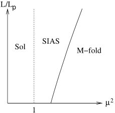
Figure 7: Phase diagram in the plane of cross-link concentration $\mu^{2}$ and polymer flexibility $L/L_{p}$. To the right of the vertical dotted line, SIAS order becomes stable, wheras M-fold order appears to the right of the continuous tilted line which depends on M.

The results of the previous sections can be summarized in a phase diagram, presented in Fig. 7. The control parameters are the cross-link density measured by $\mu^{2}$, the polymer flexibility measured by $L/L_{p}$, and the cross-linking angle $\theta$. Irrespective of the cross-linking angle, independent of the stiffness of the filaments and of the softness of the cross-links there is a continuous gelation transition accompanied by random local orientational ordering (SIAS phase) at the critical cross-link density $\mu_{c}^{2}=1$. This glassy ordering has been encountered previously for randomly linked molecules with many legs ($p$-Beine) Goldbart and Zippelius (1994); Theissen et al. (1996). The free energy of the SIAS is above the free energy of the sol, which however is unstable beyond $\mu^{2}=1$ and hence, is not available in this region of the phase diagram.

What is new, is the appearance of a state with long range orientational order, if the crossing angle $\theta=\frac{k}{M}\,2\pi$ where $k,M\in\mathbb{Z}$. This phase is characterized by a spontaneous breaking of the rotational symmetry. For sensitive cross-links the symmetry of the orientational order is $M$-fold, for unsensitive cross-links and odd $M$ the resulting phase has $2M$-fold symmetry. The free energy of the long ranged ordered state is below the free energy of the isotropic sol as well as below the free energy of the SIAS. Hence, we expect it to win as soon as it appears, even though we cannot do a complete stability analysis beyond the variational Ansatz.

We find that the appearance of long range order is pushed to higher values of $\mu^{2}$ as the constraint for the crossing angle is softened. The same effect is observed for increasing flexibility of the polymers, – because it becomes more difficult to sustain the orientation of the polymers –, and increasing $M$.

When reading the phase diagram, we should keep in mind that the parameters $\mu^{2}$ and $L/L_{p}$ are not thermodynamic ones like a temperature or a chemical potential because changing either of them changes the disorder ensemble, too. This means that two points in the phase diagram correspond effectively to two different systems.

V Conclusions - Discussion

In this paper, we studied the role of the cross-linking angle in the formation of orientational order in random networks of semiflexible polymers in two dimensions. We have used a variational Ansatz to map out a phase diagram. Besides a statistically isotropic amorphous solid (SIAS) we find more exotic gels with random positional order coexisting with long ranged orientational order, whose symmetry is dictated by the crossing angle. In analogy to liquid crystals with long range orientational order and thermal centre of mass motion like in a fluid, these gel phases might be termed “glassy crystals”– with long range orientational order and frozen in random positions like in a glass. It is interesting to note that the tetratic ordering, which corresponds to $M=4$ in our system, has been predicted and/or observed in a variety of physical systems with quite different constituents and underlying physical mechanisms Bruinsma (2001); Donev et al. (2006); Zhao et al. (2007); Narayan et al. (2006).

Because of the peculiarities of two dimensions, we expect fluctuations to affect positional localization Mermin and Wagner (1966); Goldbart et al. (2004). It is known, in the context of 2d defect-mediated melting, that at finite temperature positional order can only be quasi-long ranged whereas orientational order can be truely long ranged Nelson (2002). A study of the corresponding phenomena for our positionally amorphous and orientationally ordered system is a very interesting direction for further investigation.

We point out that the finite bending rigidity is an essential ingredient of our model. It allows the effective decoupling of positional and orientational degrees of freedom close to the gelation transition. In the case of infinitely stiff polymers on the other hand, a rigid cross-link would automatically fix both position and orientation. The nature of the emerging network is an interesting problem which goes beyond the scope of this paper.

Another possible extension of our work concerns more elaborate variational Ansätze probing the appearance of combined M-fold and glassy orientational order. Here, the chains in the gel fraction are assumeed to be orientationally localized in preferential directions which vary from chain to chain but macroscopically average in an M-fold pattern.

The three-dimensional generalization of our model has to deal with the fact that a finite cross-linking angle between two wormlike chains prescribes a cone and not a plane. If we want to describe cross-links with torsional rigidity, we need to go beyond the simple WLC model and use the helical WLC Yamakawa (1997).

In this work, we focused on orientational and glassy order in networks of semiflexible polymers mediated through appropriate cross-links. We assume that the excluded-volume interaction is such that it supports a macroscopically translationally and rotationally invariant liquid which, upon cross-linking, may give rise to ordered networks. Although this assumption is mathematically consistent and facilitates the analytical treatment of our model, it may be challenged in experimental realizations where the excluded volume may lead to lyotropic alignment in dense systems. In a future extension of our model, one may envisage adding a Maier-Saupe aligning pseudopotential as in Refs. Warner et al. (1985); Spakowitz and Wang (2003) and studying its interplay with the cross-link induced interaction.

Appendix A Evaluating expectation values - the WLC propagator

The wormlike chain propagator $G(\varphi,s_{1};\varphi^{\prime},s_{2})$ quantifies the probability that the tangential vector of monomer $s_{1}$ points into the direction $\varphi$ provided that the tangential vector of monomer $s_{2}$ points into the direction $\varphi^{\prime}$:

$$G(\varphi,s_{1};\varphi^{\prime},s_{2})$$

$$:= \Big{\langle}\delta(\varphi-\psi(s_{1}))\;\delta(\varphi^{\prime}-\psi(s_{2}))\Big{\rangle}^{{\cal H}_{WLC}}$$

$$= \frac{1}{{\cal N}}\int_{s_{1}}^{s_{2}}\!\!{\cal D}\{{\mathbf{t}}\}\;\;{\rm e}^{-\frac{\kappa}{2}\int_{s_{1}}^{s_{2}}\!{\rm d}\tau\left(\frac{{\rm d}\mathbf{t}}{{\rm d}\tau}\right)^{2}}$$

Here, ${\cal N}$ denotes the normalization and $\psi(s)$ the angle corresponding to the unity vector $\mathbf{t}(s)$. In principle, the path integral includes all the monomers from $0$ to $L$, but the monomers that lie not between $s_{1}$ and $s_{2}$ do not affect the result and can be integrated out. In order to perform the remaining path integral we write down a discretized version of the above expression replacing the continuous degrees of freedom by a finite number $l$ of them such that ${\mathbf{t}}_{1}$ corresponds to ${\mathbf{t}}(s_{1})$ and that ${\mathbf{t}}_{l}$ corresponds to ${\mathbf{t}}(s_{2})$. The distance $\epsilon$ between neighbors is determined by $l\epsilon=|s_{2}-s_{1}|$. Expressing the integral and the derivatives of the wormlike chain Hamiltonian by their discretized versions and calling the normalization constant for the discretized path integral ${\cal N}_{\epsilon}$ we arrive at Kleinert (2007)

$$G_{\epsilon} = \frac{1}{{\cal N}_{\epsilon}}\prod_{i=2}^{l-1}\!\!\left(\int\frac{{\rm d}\varphi_{i}}{2\pi}\right)\exp\left(-\frac{\kappa}{2}\epsilon\sum_{i=1}^{l-1}\left(\frac{{\mathbf{t}}_{i}-{\mathbf{t}}_{i+1}}{\epsilon}\right)^{2}\right)$$

$$= \frac{1}{{\cal N}_{\epsilon}}\prod_{i=2}^{l-1}\left(\int\frac{{\rm d}\varphi_{i}}{2\pi}\right)$$

$$\hskip 36.98866pt\exp\left(-\frac{\kappa}{\epsilon}\sum_{i=1}^{l-1}\left(1-\cos(\varphi_{i}-\varphi_{i+1})\right)\right)$$

We want now to perform the integrations over the $\varphi_{i}$. For that purpose it is convenient to decouple $\varphi_{i}$ and $\varphi_{i+1}$ by means of

$${\rm e}^{a\cos\varphi}\;=\;\sum_{q=-\infty}^{\infty}I_{q}(a)\;{\rm e}^{iq\varphi}$$

where the $I_{q}(a)$ denote modified Bessel functions. Performing the integrations we arrive at

$$G_{\epsilon}=\frac{1}{{\cal N}_{\epsilon}}\sum_{q=-\infty}^{\infty}\left({\rm e}^{-\frac{\kappa}{\epsilon}}I_{q}(\frac{\kappa}{\epsilon})\right)^{l-1}{\rm e}^{iq(\varphi_{1}-\varphi_{l})}$$

and integrating over $\frac{\varphi_{1}}{2\pi}$ and $\frac{\varphi_{l}}{2\pi}$ we find that the normalization is given by ${\cal N}_{\epsilon}=\big{(}\exp(-\kappa/\epsilon)I_{0}(\kappa/\epsilon)\big{)}^{l-1}$. Last, we take the limit $\epsilon\rightarrow 0$ keeping $l\epsilon=|s_{1}-s_{2}|$ constant. It is thus possible to express the modified Bessel functions by the asymptotic expansion $I_{q}(a)\sim\frac{\exp(a)}{\sqrt{2\pi a}}\big{(}1-\frac{4q^{2}-1}{8a}+\dots\big{)}$ and the propagator converges to

$$G(\varphi,s_{1};\varphi^{\prime},s_{2})=\!\!\sum_{q=-\infty}^{\infty}{\rm e}^{-\frac{1}{2\kappa}q^{2}|s_{1}-s_{2}|}\;{\rm e}^{iq(\varphi-\varphi^{\prime})}$$ (A.2)

Calculating a general 2-point correlation function of the (real valued) observables ${\cal O}_{1}$ and ${\cal O}_{2}$ at positions $s_{1}$ and $s_{2}$ respectively by means of the above propagator we find

$$\Big{\langle}{\cal O}_{1}(\psi(s_{1}))\;{\cal O}_{2}(\psi(s_{2}))\Big{\rangle}^{{\cal H}_{WLC}}$$

$$= \sum_{q=-\infty}^{\infty}{\rm e}^{-\frac{1}{2\kappa}q^{2}|s_{1}-s_{2}|}\;\hat{\cal O}_{1}(q)\;\hat{\cal O}_{2}^{*}(q)\;\;,$$

where $\hat{\cal O}_{1}$ and $\hat{\cal O}_{2}$ denote the Fourier transformation of the observables. We learn from this expression that only the Fourier components to the same $q$ couple to each other and that the rate of the exponential decay of correlations along the filament scales with $q^{2}$.

Appendix B Mean-field replica free energy and the saddle point equations

In order to obtain the disorder averaged free energy $[F]$ by means of the replica method we need to calculate the disorder averaged $n$-fold replicated partition function

$$[Z^{n}] \propto \sum_{M=0}^{\infty}\prod_{e=1}^{M}\left(\sum_{i_{e},j_{e}=1}^{N}\int_{s_{e},s^{\prime}_{e}}\sum_{\sigma_{e}}\right)\frac{1}{M!}\left(\frac{\mu^{2}V}{2Ny}\right)^{M}$$

$$\Big{<}\prod_{e=1}^{M}\Bigg{\{}\delta(\hat{\mathbf{r}}_{i_{e}}(s_{e})-\hat{\mathbf{r}}_{j_{e}}(s^{\prime}_{e}))\times$$

$$\hskip 14.22636pt\times\frac{{\rm e}^{\gamma\sum_{\alpha=1}^{n}\cos(\psi^{\alpha}_{i_{e}}(s_{e})-\psi^{\alpha}_{j_{e}}(s^{\prime}_{e})-\theta_{\sigma_{e}})}}{I_{0}^{n}(\gamma)}\Bigg{\}}\Big{>}_{n+1}^{{\cal H}}$$

where ${\mathbf{r}}^{\alpha}_{i}(s)$ and $\psi^{\alpha}_{i}(s)$ denote the position vector and angle of orientation of segment $s$ belonging to polymer $i$ inside the $\alpha$th replica. For sensitive cross-links $\theta_{\sigma}$ equals always the single crossing-angle $\theta$, i.e. the normalization $y=1$, and we can omit the summation over $\sigma$, but in the unsensitive case $\theta_{\sigma}$ takes the two values $\theta_{1}=\theta$ and $\theta_{2}=\theta+\pi$ and so, $y=2$.

Observing that the formula factorizes in the cross-link index $e$ it is possible to perform the sum over the number of cross-links $M$ that leads to an exponential function

$$[Z^{n}] \propto \Bigg{<}\exp\Bigg{(}\frac{\mu^{2}V}{2N}\sum_{i,j=1}^{N}\int_{s,s^{\prime}}\;\delta(\hat{\mathbf{r}}_{i}(s)-\hat{\mathbf{r}}_{j}(s^{\prime}))\times$$

$$\hskip 85.35826pt\times\Delta(\check{\psi}_{i}(s)-\check{\psi}_{j}(s^{\prime}),\theta)\Bigg{)}\Bigg{>}^{{\cal H}}_{n+1}\;$$

where for sensitive cross-links the function $\Delta$ is defined as

$$\Delta_{s}(\check{\psi},\theta)\equiv\frac{{\rm e}^{\gamma\sum_{\alpha=1}^{n}\cos(\psi^{\alpha}-\theta)}}{I_{0}^{n}(\gamma)}$$ (B.5)

and in the unsensitive case on the other hand as

$$\Delta_{u}(\check{\psi},\theta)\equiv\frac{1}{2}\!\!\left\{\frac{{\rm e}^{\gamma\sum_{\alpha}\!\!\cos(\psi^{\alpha}-\theta)}}{I_{0}^{n}(\gamma)}+\frac{{\rm e}^{\gamma\sum_{\alpha}\!\!\cos(\psi^{\alpha}-(\theta+\pi))}}{I_{0}^{n}(\gamma)}\right\}\;.$$ (B.6)

After the disorder average, all the sites, i.e. all the polymer segments, are equivalent but still appear explicitly, coupled by the cross-linking constraint $\Delta$ and the delta functions. Expressing the delta functions in Fourier space we can rewrite our formula in terms of the quantity

$$Q(\hat{\mathbf{k}},\check{m})=\frac{1}{N}\sum_{i=1}^{N}\int_{s}{\rm e}^{i\hat{\mathbf{k}}\hat{\mathbf{r}}_{i}(s)}\;{\rm e}^{i\check{m}\check{\psi}_{i}(s)}$$

Using this definition and writing ${\cal H}_{ev}$ explicitly the replicated partition function reads

$$[Z^{n}] \propto \bigg{\langle}\exp\Big{(}\frac{\mu^{2}N}{2V^{n}}\sum_{\hat{\mathbf{k}},\check{m}}\Delta_{\check{m}}\;|Q(\hat{\mathbf{k}},\check{m})|^{2}\Big{)}$$

$$\hskip 9.95845pt\exp\Big{(}-\!\!\frac{\lambda^{2}N^{2}}{2V}\sum_{\alpha=0}^{n}\sum_{{\mathbf{k}}\neq 0}\sum_{m}|\rho^{\alpha}({\mathbf{k}},m)|^{2}\bigg{\rangle}_{n+1}^{{\cal H}_{WLC}}.$$

In section II the parameter $\lambda^{2}$ was introduced in its most general form depending on $|\mathbf{k}|$ and $m$, but as it turns out a constant is sufficient for our purpose and allows in the following for a more compact notation. Because of the symmetry $|Q(\hat{\mathbf{k}},\check{m})|^{2}=|Q(-\hat{\mathbf{k}},-\check{m})|^{2}$ it is only the real part of $\Delta_{\check{m}}$ that contributes and we thus redefine the sensitive kernel $\Delta_{s}$ accordingly as

$$\Delta_{s,\check{m}}=\frac{\prod_{\alpha=1}^{n}I_{m^{\alpha}}(\gamma)}{I^{n}_{0}(\gamma)}\cos\Big{(}\sum_{\alpha}m^{\alpha}\theta\Big{)}.$$ (B.7)

For unsensitive cross-links $\Delta_{u,\check{m}}$ equals zero if the sum $\sum_{\alpha=1}^{n}m^{\alpha}$ is not even, but takes otherwise the values of the sensitive kernel in (B.7).

We are now going to rearrange the contributions of intra-polymer repulsion and Deam-Edwards distribution into contributions belonging to the following subsets of the space of $(n+1)$-fold replicated vectors $\hat{\mathbf{k}}$:

• The $0$-replica sector (0RS) consisting only of $\hat{0}$

• The $1$-replica sector (1RS) including all vectors of the form $\hat{\mathbf{k}}=(\vec{0},\dots,{\mathbf{k}}^{\alpha},\dots,\vec{0})$ where ${\mathbf{k}}^{\alpha}\neq 0$

• The higher-replica sector (HRS) containing all the $\hat{\mathbf{k}}$ where wave vectors in at least to replicas are non-zero, i.e. there are $\alpha\neq\beta\in\{0,1,\dots,n\}$ with ${\mathbf{k}}^{\alpha}\neq 0$ and ${\mathbf{k}}^{\beta}\neq 0$

In the following we denote the sum over 0RS and HRS by $\overline{\sum}_{\hat{\mathbf{k}}}$ and the sum over the 1RS as $\tilde{\sum}_{{\mathbf{k}}}$. For the 1RS we obtain the new kernel

$$\tilde{\Delta}_{\check{m}}^{\alpha}=\frac{\lambda^{2}N}{2V}\prod_{\beta\neq\alpha=1}^{n}\delta_{m^{\beta},0}-\frac{\mu^{2}}{2V^{n}}\;\Delta_{\check{m}}$$ (B.8)

Using $\tilde{Q}^{\alpha}({\mathbf{k}},\check{m})$ as shorthand notation for $Q(\hat{\mathbf{k}},\check{m})$ when only the wave vector ${\mathbf{k}}^{\alpha}$ in replica $\alpha$ is non-zero the expression reads

$$[Z^{n}] \propto \bigg{\langle}\exp\Big{(}-N\sum_{\alpha=0}^{n}\tilde{\sum}_{{\mathbf{k}},\check{m}}\tilde{\Delta}_{\check{m}}^{\alpha}\;|\tilde{Q}^{\alpha}({\mathbf{k}},\check{m})|^{2}\Big{)}$$

$$\hskip 11.38109pt\exp\Big{(}\frac{\mu^{2}N}{2V^{n}}\overline{\sum}_{\hat{\mathbf{k}},\check{m}}\Delta_{\check{m}}\;|Q(\hat{\mathbf{k}},\check{m})|^{2}\Big{)}\bigg{\rangle}_{n+1}^{{\cal H}_{WLC}}.$$

In order to decouple the sites we are now going to apply a Hubbard-Stratonovich transformation. The symmetry $Q(\hat{\mathbf{k}},\check{m})=Q^{*}(-\hat{\mathbf{k}},-\check{m})$ and the analogous relation for $\tilde{Q}^{\alpha}({\mathbf{k}},\check{m})$ have to be reflected by their corresponding fields $\Omega(\hat{\mathbf{k}},\check{m})$ and $\tilde{\Omega}^{\alpha}({\mathbf{k}},\check{m})$. After the transformation $[Z^{n}]$ can be written as

$$[Z^{n}]\propto\int{\cal D}\{\tilde{\Omega}^{\alpha},\Omega\}\exp\left(-N{\cal F}(\{\tilde{\Omega}^{\alpha},\Omega\})\right)$$ (B.9)

where the integrals over the complex fields are meant to be integrations over real and imaginary parts separately. The replica free energy ${\cal F}$ is given by

$${\cal F} = \sum_{\alpha=0}^{n}\tilde{\sum}_{{\mathbf{k}}}\sum_{\check{m}}|\tilde{\Omega}^{\alpha}|^{2}+\frac{\mu^{2}}{2V^{n}}\overline{\sum}_{\hat{\mathbf{k}}}\sum_{\check{m}}|\Omega|^{2}$$

$$-\ln\Bigg{\langle}\exp\bigg{(}2i\sum_{\alpha=0}^{n}\tilde{\sum}_{{\mathbf{k}}}\sum_{\check{m}}\sqrt{\tilde{\Delta}}\;\Re\,\Big{(}\tilde{\Omega}^{\alpha}\;\int_{s}$$

$$\hskip 28.45274pt\exp\Big{\{}-i{\mathbf{k}}^{\alpha}{\mathbf{r}}^{\alpha}(s)\Big{\}}\exp\Big{\{}-i\check{m}\check{\psi}(s)\Big{\}}\Big{)}$$

$$\hskip 22.76228pt+\frac{\mu^{2}}{V^{n}}\overline{\sum}_{\hat{\mathbf{k}}}\sum_{\check{m}}\sqrt{\Delta}\;\Re\,\Big{(}\Omega\;\int_{s}$$

$$\hskip 28.45274pt\exp\Big{\{}-i\hat{\mathbf{k}}\hat{\mathbf{r}}(s)\Big{\}}\exp\Big{\{}-i\check{m}\check{\psi}(s)\Big{\}}\Big{)}\bigg{)}\Bigg{\rangle}^{{\cal H}_{WLC}}_{n+1}$$

Using the saddle point approximation we replace the integral (B.9) by its maximal contribution. The corresponding values of the order parameter fields have to fulfill the self-consistency equations that arise from

$$\frac{\partial{\cal F}}{\partial\Re\tilde{\Omega}^{\alpha}({\mathbf{k}}_{0},\check{m}_{0})}=0\; \frac{\partial{\cal F}}{\partial\Im\tilde{\Omega}^{\alpha}({\mathbf{k}}_{0},\check{m}_{0})}=0,$$ ,

$$\frac{\partial{\cal F}}{\partial\Re\Omega(\hat{\mathbf{k}}_{0},\check{m}_{0})}=0\; \;\frac{\partial{\cal F}}{\partial\Im\Omega(\hat{\mathbf{k}}_{0},\check{m}_{0})}=0.$$ and

Note that there are many ways to perform the HS transformation, each of them leading to a different replica free energy ${\cal F}$. The resulting saddle-point replica free energy on the other hand is always the same as it can be checked easily. As a consequence, we are free to redefine the fields for later convenience by doing the replacements $\Re\Omega(\hat{\mathbf{k}},\check{m})\rightarrow\sqrt{\Delta_{\check{m}}}\;\Re\Omega(\hat{\mathbf{k}},\check{m})$ and for the imaginary part accordingly. The advantage of this transformation is that the saddle-point fields $\Omega_{SP}(\hat{\mathbf{k}},\check{m})$ are now directly related to an expectation value of $Q(\hat{\mathbf{k}},\check{m})$ as presented in the main part, equation (12). This connection between $Q$ and its corresponding field $\Omega$ is derived by means of an external field that couples to $Q$. Performing then the Hubbard-Stratonovich transformation and taking the logarithmic derivatives with respect to real and imaginary part of the field on both sides of the equation, i.e. for both the microscopic and the field theoretic representation of our theory, results in the desired relation between $Q$ and $\Omega$.

The 0RS/HRS part of the free energy in terms of the new fields reads then

$${\cal F} = \frac{\mu^{2}}{2V^{n}}\overline{\sum}_{\hat{\mathbf{k}}}\sum_{\check{m}}\Delta|\Omega|^{2}$$

$$-\ln\Bigg{\langle}\exp\bigg{(}\frac{\mu^{2}}{V^{n}}\overline{\sum}_{\hat{\mathbf{k}}}\sum_{\check{m}}\Delta\;\Re\,\Big{(}\Omega\;\int_{s}$$

$$\hskip 28.45274pt\exp\Big{\{}-i\hat{\mathbf{k}}\hat{\mathbf{r}}(s)\Big{\}}\exp\Big{\{}-i\check{m}\check{\psi}(s)\Big{\}}\Big{)}\bigg{)}\Bigg{\rangle}^{{\cal H}_{WLC}}_{n+1}$$

The 1RS part is treated in the next section.

Appendix C Stability of the 1-replica sector

The fields of the 1-replica sector, $\tilde{\Omega}^{\alpha}({\mathbf{k}},\check{m})$, can be subdivided into the fields where $\check{m}$ is such that only the entry $m^{\alpha}$ is non-vanishing and those corresponding to the other possible values of $\check{m}$. In the former case the fields describe $M$-fold orientationally symmetric density fluctuations with wave vector ${\mathbf{k}}$ in replica $\alpha$ and have thus a clear physical meaning. The other fields break replica symmetry in the sense that they describe density fluctuations e.g. in replica $\alpha$ accompanied by purely orientational fluctuations in other replicas. These fields are unphysical and need thus to equal zero.

In order to study the stability of the 1RS with respect to fluctuations in the physical fields $\rho^{\alpha}({\mathbf{k}},m)$ it is sufficient to study stability for one replica only. The expansion of the corresponding free energy reads up to second order

$${\cal F}_{1RS}=\tilde{\sum}_{{\mathbf{k}}}\sum_{m}|\tilde{\rho}({\mathbf{k}},m)|^{2}$$ (C.12)

$$\hskip 14.22636pt+2\tilde{\sum}_{{\mathbf{k}}_{1},{\mathbf{k}}_{2}}\sum_{m_{1},m_{2}}\tilde{\rho}({\mathbf{k}}_{1},m_{1})\tilde{\rho}({\mathbf{k}}_{2},m_{2})$$

$$\hskip 17.07164pt\sqrt{\tilde{\Delta}}_{m_{1}}\sqrt{\tilde{\Delta}}_{m_{2}}\underbrace{\int_{s_{1},s_{2}}\left\langle{{\rm e}^{i({\mathbf{k}}_{1}{\mathbf{r}}_{1}+{\mathbf{k}}_{2}{\mathbf{r}}_{2})}{\rm e}^{i(m_{1}\psi_{1}+m_{2}\psi_{2})}}\right\rangle}_{{\cal C}({\mathbf{k}}_{1},{\mathbf{k}}_{2};m_{1},m_{2})}$$

with $\mathbf{r}_{x}:=\mathbf{r}(s_{x})$ and $\psi_{x}:=\psi(s_{x})$. Choosing $\lambda^{2}>\mu^{2}$ the kernel $\tilde{\Delta}_{m}=\frac{\lambda^{2}}{2}-\frac{\mu^{2}}{2}\frac{I_{m}(\gamma)}{I_{0}(\gamma)}\cos(m\theta)$ is positive because $\frac{I_{m}(\gamma)}{I_{0}(\gamma)}\leq 1$. It is thus possible to redefine the fields by introducing $\overline{\rho}({\mathbf{k}},m):=\sqrt{\Delta_{m}}\tilde{\rho}({\mathbf{k}},m)$ without changing the stability. The corresponding free energy is given by

$$\overline{\cal F}_{1RS}=\tilde{\sum}_{{\mathbf{k}}}\sum_{m}\frac{2}{\lambda^{2}-\mu^{2}\frac{I_{m}(\gamma)}{I_{0}(\gamma)}\cos(m\theta)}|\overline{\rho}({\mathbf{k}},m)|^{2}$$ (C.13)

$$\hskip 2.84526pt+2\tilde{\sum}_{{\mathbf{k}}_{1},{\mathbf{k}}_{2}}\sum_{m_{1},m_{2}}\overline{\rho}({\mathbf{k}}_{1},m_{1})\overline{\rho}({\mathbf{k}}_{2},m_{2}){\cal C}({\mathbf{k}}_{1},{\mathbf{k}}_{2};m_{1},m_{2})$$

Let us now consider the two contributions to $\overline{\cal F}_{1RS}$ separately: It is evident that the first term is a positive quadratic form provided that $\lambda^{2}$ is large enough. If we consider stiff rods as the limiting case of very unflexible wormlike chains the matrix of the second quadratic form can be diagonalized by switching back from the Fourier modes $m$ to the real space variables $\varphi$. Writing ${\mathbf{r}}(s)={\mathbf{r}}_{0}+s{\mathbf{t}}$ and integrating over ${\mathbf{r}}_{0}$ and ${\mathbf{t}}$ we find for ${\cal C}$

$$\int_{s_{1},s_{2}}\Big{\langle}{\rm e}^{i({\mathbf{k}}_{1}{\mathbf{r}}_{1}+{\mathbf{k}}_{2}{\mathbf{r}}_{2})}\;\delta(\varphi_{1}-\psi_{1})\delta\left(\varphi_{2}-\psi_{2}\right)\Big{\rangle}$$ (C.14)

$$= \delta_{{\mathbf{k}}_{1},-{\mathbf{k}}_{2}}\;\delta(\varphi_{1}-\varphi_{2})\;\frac{\sin^{2}({\mathbf{k}}_{1}{\mathbf{t}}_{1}/2)}{\left({\mathbf{k}}_{1}{\mathbf{t}}_{1}/2\right)^{2}}$$

and know thus that the second quadratic form is positive semi-definite. Altogether we have thus proved stability in the case of stiff rods, but we assume that this result will at least hold for wormlike chains with large $L/L_{p}$, too.

Appendix D Variational free energy: M-fold symmetric long ranged order

In this Appendix, we present some details on the derivation of the variational free energy (IV.1.1) of the M-fold orientationally ordered amorphous solid. We insert the corresponding replica order parameter Ansatz (24) into the general replica free energy (IV) and expand it in powers the variational parameters $\frac{1}{\xi^{2}}$ and $\eta$.

D.1 Gaussian part

The Gaussian part reads

$$f_{G} = \frac{\mu^{2}Q^{2}}{2V^{n}}\sum_{\hat{\mathbf{k}}}\delta_{\sum_{\alpha=0}^{n}{\mathbf{k}}^{\alpha},0}{\rm e}^{-\xi^{2}\hat{\mathbf{k}}^{2}}\int_{\check{\varphi}_{1},\check{\varphi}_{2}}\;\Delta(\check{\varphi}_{1},\check{\varphi}_{2})$$

$$\frac{1}{I_{0}^{2n}(\eta)}{\rm e}^{\eta\sum_{\alpha=1}^{n}(\cos(M\varphi_{1}^{\alpha})+\cos(M\varphi_{2}^{\alpha}))}\quad.$$

The spatial part is easily computed by replacing the sum over the replicated Fourier variables $\hat{\mathbf{k}}$ by an integral and representing the delta function in Fourier space. Performing the resulting integrations we arrive at

$$f_{G}=\frac{1}{n+1}\left(\frac{1}{4\pi\xi^{2}}\right)^{n}f_{0}\;.$$

For the orientational contribution $f_{o}$ we find

$$f_{o}$$

$$= \int_{\check{\varphi}_{1},\check{\varphi}_{2}}\;\Delta(\check{\varphi}_{1}-\check{\varphi}_{2},\theta)\frac{{\rm e}^{\eta\sum_{\alpha=1}^{n}(\cos(M\varphi_{1}^{\alpha})+\cos(M\varphi_{2}^{\alpha}))}}{I_{0}^{2n}(\eta)}$$

$$\sim 1+n\ln\left(\int_{\varphi_{1},\varphi_{2}}\Delta(\varphi_{1}-\varphi_{2},\theta)\frac{{\rm e}^{\eta(\cos(M\varphi_{1})+\cos(M\varphi_{2}))}}{I_{0}^{2}(\eta)}\right)$$

$$= 1+n\ln\Big{(}1+2\sum_{q=1}^{\infty}\frac{I_{q}^{2}(\eta)}{I_{0}^{2}(\eta)}\frac{I_{Mq}(\gamma)}{I_{0}(\gamma)}\cos(Mq\theta)\Big{)}\quad.$$

For $\theta=\frac{k}{M}2\pi$ the cosine equals $1$ and vanishes. In order to obtain the last line we replaced the three functions depending on the $\varphi$’s by their Fourier representations. Performing then the integrations lead to Kronecker Deltas that cancel two of the three sums over Fourier modes.

Altogether we find for the Gaussian contribution in linear order in the replica index $n$

$$f_{G}=\frac{\mu^{2}Q^{2}}{2}\Big{\{}-1-\ln(4\pi\xi^{2})+\ln\Big{(}1+2\sum_{q=1}^{\infty}\frac{I_{q}^{2}(\eta)}{I_{0}^{2}(\eta)}\frac{I_{Mq}(\gamma)}{I_{0}(\gamma)}\Big{)}\Big{\}}.$$

Considering unsensitive crosslinker the corresponding expression reads

$$f_{o}=1+n\ln\Big{(}1+2\sum_{q=1}^{\infty}\;\delta_{Mq,2\mathbb{Z}}\;\frac{I_{q}^{2}(\eta)}{I_{0}^{2}(\eta)}\frac{I_{Mq}(\gamma)}{I_{0}(\gamma)}\cos(Mq\theta)\Big{)}\quad,$$ (D.16)

i.e. for odd $M$ the contributions corresponding to odd $q$ are projected out. For $M$ even on the other hand, we obtain the same result as for the sensitive cross-links.

Note that for hard crosslinks ($\gamma=\infty$) there is an alternative expression for the $f_{o}$. For sensitive cross-links it is given by

$$f_{o}$$

$$\sim 1+n\ln\left(\int_{\varphi_{1},\varphi_{2}}\Delta(\varphi_{1}-\varphi_{2},\theta)\frac{{\rm e}^{\eta(\cos(M\varphi_{1})+\cos(M\varphi_{2}))}}{I_{0}^{2}(\eta)}\right)$$

$$\sim 1+n\ln\left(\frac{1}{I_{0}^{2}(\eta)}\int_{\varphi}{\rm e}^{\eta(\cos(M(\varphi+\theta))+\cos(M\varphi))}\right)$$

$$\sim 1+n\ln\left(\frac{1}{I_{0}^{2}(\eta)}\int_{\varphi}{\rm e}^{2\eta(\cos(M\varphi+\frac{M\theta}{2}))\cos(\frac{M\theta}{2}))}\right)$$

$$\sim 1+n\ln\left(\frac{I_{0}(2\eta\cos(\frac{M\theta}{2}))}{I_{0}^{2}(\eta)}\right)$$

and in the unsensitive case we have

$$f_{o}\sim 1+n\ln\Bigg{(}\frac{1}{I_{0}^{2}(\eta)}\frac{1}{2}\bigg{\{} I_{0}\big{(}2\eta\cos(\frac{M\theta}{2})\big{)}$$

$$+I_{0}\big{(}2\eta\cos(\frac{M(\theta+\pi)}{2})\big{)}\bigg{\}}\Bigg{)}\quad.$$

D.2 Log-trace contributions

Let us now turn to the log-trace contribution that we will expand up to the third order in the gel fraction $Q$:

$$f_{lt} = \mu^{2}Qf_{lt,1}+\frac{\mu^{4}Q^{2}}{2}\Big{(}f_{lt,2}-f_{lt,1}^{2}\Big{)}$$

$$+\frac{\mu^{6}Q^{3}}{6}\Big{(}f_{lt,3}+2f_{lt,1}^{3}-3f_{lt,1}f_{lt,2}\Big{)}+{\cal O}(Q^{4}).$$

The first-order term gives a trivial contribution because of

$$f_{lt,1}$$

$$= \Bigg{<}\frac{1}{V^{n}}\;\overline{\sum}_{\hat{\mathbf{k}}}\int_{\check{\varphi},\check{\varphi}^{\prime}}\delta_{{\mathbf{0}},\sum_{\alpha=0}^{n}\mathbf{k}^{\alpha}}\;{\rm e}^{-\xi^{2}{\hat{\mathbf{k}}}^{2}}\times$$

$$\hskip 11.38092pt\times\frac{{\rm e}^{\gamma\sum_{\alpha=1}^{n}\cos(\varphi^{\alpha}-\varphi^{\prime\alpha}-\theta)}}{I_{0}^{n}(\gamma)}\frac{{\rm e}^{\eta\sum_{\alpha}\cos(m\varphi^{\prime\alpha})}}{{\rm I}_{0}^{n}(\eta)}\times$$

$$\hskip 85.35826pt\times\int_{s}\;{\rm e}^{i\hat{\mathbf{k}}\hat{\mathbf{r}}(s)}\delta(\check{\varphi}^{\prime}-\check{\psi}(s))\Bigg{>}$$

$$= \frac{1}{V^{n}}\int_{s}\Bigg{<}\int_{\check{\varphi}}\frac{{\rm e}^{\gamma\sum_{\alpha=1}^{n}\cos(\varphi^{\alpha}-\psi(s)^{\alpha}-\theta)}}{I_{0}^{n}(\gamma)}\frac{{\rm e}^{\eta\sum_{\alpha}\cos(m\varphi^{\alpha})}}{{\rm I}_{0}^{n}(\eta)}\Bigg{>}$$

$$= \frac{1}{V^{n}}\;.$$

In the second step we use $\hat{\mathbf{r}}(s)=\hat{\mathbf{r}}(0)+\int_{0}^{s}{\rm d}\tau\;\hat{\mathbf{t}}(\tau)$ and transform the original path integral ${\cal D}\{\hat{\mathbf{r}}(s)\}$ into an integral $\frac{{\rm d}\hat{\mathbf{r}}(0)}{V^{n+1}}$ and a path integral ${\cal D}\{\hat{\psi}(s)\}$ over angular variables. Performing the $\hat{\mathbf{r}}(0)$ integration we get a Kronecker delta setting $\hat{\mathbf{k}}$ to zero. The last line follows from the fact that the functions are normalized and the two integrations with respect to $\check{\varphi}$ and $\check{\psi}(s)$ simply lead to $1$.

The second-order contribution reads

$$f_{lt,2} = \frac{1}{V^{2n}}\int_{s_{1},s_{2}}\Bigg{<}\overline{\sum}_{\hat{\mathbf{k}}_{1}}\overline{\sum}_{\hat{\mathbf{k}}_{2}}\delta_{{\mathbf{0}},\sum_{\alpha=0}^{n}\mathbf{k}_{1}^{\alpha}}\;\delta_{{\mathbf{0}},\sum_{\alpha=0}^{n}\mathbf{k}_{2}^{\alpha}}\;{\rm e}^{-\xi^{2}\left({\hat{\mathbf{k}_{1}}}^{2}+{\hat{\mathbf{k}_{2}}}^{2}\right)/2}{\rm e}^{i\left(\hat{\mathbf{k}_{1}}\hat{\mathbf{r}}(s_{1})+\hat{\mathbf{k}_{2}}\hat{\mathbf{r}}(s_{2})\right)}$$

$$\hskip 28.45274pt\int_{\check{\varphi}_{1}\check{\varphi}_{1}^{\prime}}\int_{\check{\varphi}_{2}\check{\varphi}_{2}^{\prime}}\Delta\left(\check{\varphi}_{1}-\check{\varphi}_{1}^{\prime},\theta\right)\Delta\left(\check{\varphi}_{2}-\check{\varphi}_{2}^{\prime},\theta\right)\;\delta(\check{\varphi}_{1}^{\prime}-\check{\psi}(s_{1}))\;\delta(\check{\varphi}_{2}^{\prime}-\check{\psi}(s_{2}))\;\frac{{\rm e}^{\eta\sum_{\alpha=1}^{n}\{\cos(M\varphi^{\alpha}_{1})+\cos(M\varphi^{\alpha}_{2})\}}}{{\rm I}_{0}^{2n}(\eta)}\Bigg{>}.$$

Before Taylor expanding the expression in the variational parameters, we need to perform the summations over $\hat{\mathbf{k}}_{1}$ and $\hat{\mathbf{k}}_{2}$. We integrate over ${\rm d}\hat{\mathbf{r}}(0)$ as before and get a Kronecker Delta imposing $\hat{\mathbf{k}}_{1}=-\hat{\mathbf{k}}_{2}$. There is thus only one summation left. We replace this sum by an integral and represent the Kronecker delta in Fourier space. After the two Gaussian integrations we find

$$f_{lt,2} = \;\frac{1}{V^{n}}\left(\frac{1}{4\pi\xi^{2}}\right)^{n}\frac{1}{n+1}\int_{s_{1},s_{2}}$$

$$\Bigg{<}{\rm e}^{\frac{1}{4\xi^{2}}\left(\frac{1}{n+1}\sum_{\alpha\beta=0}^{n}{\mathbf{f}}^{\alpha}{\mathbf{f}}^{\beta}-\sum_{\alpha=0}^{n}({\mathbf{f}}^{\alpha})^{2}\right)}\times$$

$$\hskip 8.53581pt\times\int_{\check{\Delta\varphi_{1}},\check{\Delta\varphi_{2}}}\frac{{\rm e}^{\gamma\sum_{\alpha=1}^{n}\big{(}\cos(\Delta\varphi_{1}^{\alpha})+\cos(\Delta\varphi_{2}^{\alpha})\big{)}}}{I_{0}^{2n}(\gamma)}\times$$

$$\hskip 8.53581pt\times\;\frac{{\rm e}^{\eta\sum_{\alpha=1}^{n}\{\cos(M(\psi_{1}^{\alpha}+\Delta\varphi_{1}^{\alpha}))+\cos(M(\psi_{2}^{\alpha}+\Delta\varphi_{2}^{\alpha}))\}}}{{\rm I}_{0}^{2n}(\eta)}\Bigg{>}$$

using the shorthand notations ${\mathbf{f}}^{\alpha}\equiv\int_{s_{1}}^{s_{2}}{\rm d}s\;{\mathbf{t}}^{\alpha}(s)$ and $\psi_{i}^{\alpha}:=\psi^{\alpha}(s_{i})$. This expression can be expanded up to the desired order and the remaining task then consists in calculating the corresponding correlation functions. Details are given in Appendix F.

For the calculation of the third-order term, we proceed the same way as before and need thus to perform three sums over wave vectors. With the abbreviation ${\mathbf{f}}_{l}^{\alpha}\equiv\int_{s_{3}}^{s_{l}}{\rm d}\tau\;{\mathbf{t}}^{\alpha}(\tau)$ the result reads

$$f_{lt,3} = \frac{1}{V^{n}}\left(\frac{1}{4\pi\xi^{2}}\right)^{n}\left(\frac{1}{3\pi\xi^{2}}\right)^{n}\left(\frac{1}{n+1}\right)^{2}\int_{s_{1},s_{2},s_{3}}$$

$$\Bigg{\langle}\exp\Bigg{\{}\frac{1}{3\xi^{2}}\bigg{(}\frac{1}{n+1}\sum_{\alpha,\beta=0}^{n}\big{(}{\mathbf{f}}_{1}^{\alpha}{\mathbf{f}}_{1}^{\beta}+{\mathbf{f}}_{2}^{\alpha}{\mathbf{f}}_{2}^{\beta}+{\mathbf{f}}_{1}^{\alpha}{\mathbf{f}}_{2}^{\beta}\big{)}-\sum_{\alpha=0}^{n}\big{(}({\mathbf{f}}_{1}^{\alpha})^{2}+({\mathbf{f}}_{2}^{\alpha})^{2}+{\mathbf{f}}_{1}^{\alpha}{\mathbf{f}}_{2}^{\alpha}\big{)}\bigg{)}\Bigg{\}}\times$$

$$\times\int_{\check{\Delta\varphi_{1}},\check{\Delta\varphi_{2}},\check{\Delta\varphi_{3}}}\frac{{\rm e}^{\gamma\sum_{\alpha=1}^{n}\big{(}\cos(\Delta\varphi_{1}^{\alpha})+\cos(\Delta\varphi_{2}^{\alpha})+\cos(\Delta\varphi_{3}^{\alpha})\big{)}}}{I_{0}^{3n}(\gamma)}\;\frac{{\rm e}^{\eta\sum_{\alpha=1}^{n}\{\cos(M(\psi_{1}^{\alpha}+\Delta\varphi_{1}^{\alpha}))+\cos(M(\psi_{2}^{\alpha}+\Delta\varphi_{2}^{\alpha}))+\cos(M(\psi_{3}^{\alpha}+\Delta\varphi_{3}^{\alpha}))\}}}{{\rm I}_{0}^{3n}(\eta)}\Bigg{>}\;.$$

Appendix E Variational free energy: SIAS

E.1 Gaussian part

In the following, we present the derivation of the SIAS variational free energy. Let us first turn to the Gaussian contribution. It is given by

$$f_{g} = \frac{\mu^{2}Q^{2}}{2V^{n}}\sum_{\hat{\mathbf{k}}}\delta_{{\mathbf{0}},\sum_{\alpha=0}^{n}\mathbf{k}^{\alpha}}{\rm e}^{-\xi^{2}{\hat{\mathbf{k}}}^{2}}\times$$

$$\times\int_{\check{\varphi},\check{\varphi}^{\prime}}\Delta(\check{\varphi}-\check{\varphi}^{\prime},\theta)\;\frac{{\rm I}_{0}(\eta|\sum_{\alpha=1}^{n}{\mathbf{u}}^{\alpha}|){\rm I}_{0}(\eta|\sum_{\alpha=1}^{n}{\mathbf{u}}^{\prime\alpha}|)}{{\rm I}_{0}^{2n}(\eta)}$$

where $\mathbf{u}^{\alpha}=(\cos\varphi^{\alpha},\sin\varphi^{\alpha})$. The spatial part is treated the same way as for the M-fold case, but the orientational contribution is slightly more complicated because it does not factorize in the replica index. By means of the integral representation of the Bessel function,

$$I_{0}(\eta)=\frac{1}{2\pi}\int_{0}^{2\pi}{\rm d}\vartheta\;{\rm e}^{\eta\cos\vartheta},$$ (E.24)

we get a factorizing expression and find in linear order in $n$ for the orientational part of the free energy

$$f_{o} = 1+n\int_{\vartheta_{1},\vartheta_{2}}\ln\Big{(}\int_{\varphi_{1},\varphi_{2}}\Delta(\varphi_{1}-\varphi_{2},\theta)\times$$

$$\hskip 71.13188pt\times\frac{1}{I_{0}^{2}(\eta)}{\rm e}^{\eta(\cos(\varphi_{1}+\vartheta_{1})+\cos(\varphi_{2}+\vartheta_{2})}\Big{)}$$

$$= 1+n\int_{\vartheta}\ln\Bigg{(}1+2\sum_{q\in\mathbb{N}}\frac{I_{q}^{2}(\eta)}{I_{0}^{2}(\eta)}\frac{I_{q}(\gamma)}{I_{0}(\gamma)}\cos(\vartheta)\Bigg{)}\;.$$

In order to obtain the last line, we simply switch from the angular variables to Fourier space. The expression is then easily expanded up to the desired order.

E.2 Log-trace contributions

The first-order contribution of the log-trace part gives the same (trivial) result as for the long range ordered case. As for the second and third order term, we again have to perform the $\hat{\mathbf{k}}$ summations first, but this calculation is done exactly the same way as before.The corresponding results are obtained from those of the M-fold case by simply replacing the M-fold orientational distributions in (D.2) and (D.2) by the corresponding SIAS distributions.

Details on the calculation of the individual terms of the second order log-trace contribution are given in Appendix G.

Appendix F Evaluation of the expectation values: M-fold

In our expansion we include all the terms up to first order in $\frac{1}{\xi^{2}}$ and up to sixth order in $\eta$.

F.1 Spatial part

Let us consider the calculation of the $\frac{1}{\xi^{2}}$-term:

$$\int_{s_{1},s_{2}}\left(\frac{1}{n+1}\sum_{\alpha,\beta=0}^{n}\left\langle{{\mathbf{f}}^{\alpha}{\mathbf{f}}^{\beta}}\right\rangle-\sum_{\alpha=0}^{n}\left\langle{({\mathbf{f}}^{\alpha})^{2}}\right\rangle\right)$$ (F.26)

$$= -n\;\int_{s_{1},s_{2}}\int_{s_{1}}^{s_{2}}{\rm d}\tau\int_{s_{1}}^{s_{2}}{\rm d}\tau^{\prime}\;\left\langle{{\mathbf{t}}(\tau){\mathbf{t}}(\tau^{\prime})}\right\rangle$$

$$= -n\;\int_{s_{1},s_{2}}\int_{s_{1}}^{s_{2}}{\rm d}\tau\int_{s_{1}}^{s_{2}}{\rm d}\tau^{\prime}\;{\rm e}^{-\frac{1}{2\kappa}|\tau-\tau^{\prime}|}$$

$$=: -nL^{2}\;g(\frac{L}{L_{p}})$$

The first expectation value gives a contribution for $\alpha=\beta$ only. Combining the two terms and noticing that each replica gives the same contribution we obtain the prefactor of $-n$. It is interesting to note that the function $g$ is closely related to the radius of gyration $R_{g}$.

$$R_{g}^{2} := \frac{1}{2}\int_{s_{1},s_{2}}\left\langle{\left(\mathbf{r}(s_{1})-\mathbf{r}(s_{2})\right)^{2}}\right\rangle$$

$$= \frac{1}{2}\int_{s_{1},s_{2}}\int_{s_{2}}^{s_{1}}{\rm d}\tau{\rm d}\tau^{\prime}\left\langle{\mathbf{t}(\tau)\mathbf{t}(\tau^{\prime})}\right\rangle$$

$$= \frac{L^{2}}{2}\;g(\frac{L}{L_{p}})$$

F.2 Coupling terms

In order to calculate the lowest order coupling terms we expand the spatial part in first order. For $\theta=\frac{k}{M}2\pi$ we find

$$\frac{1}{4\xi^{2}}\Bigg{\langle}\Big{\{}\frac{1}{n+1}\sum_{\alpha\neq\beta=0}^{n}\mathbf{f}^{\alpha}\mathbf{f}^{\beta}-\frac{n}{n+1}\sum_{\alpha=0}^{n}\left(\mathbf{f}^{\alpha}\right)^{2}\Big{\}}\times$$ (F.28)

$$\hskip 28.45274pt\times\int_{\check{\Delta\varphi_{1}},\check{\Delta\varphi_{2}}}\frac{{\rm e}^{\gamma\sum_{\alpha=1}^{n}(\cos\Delta\varphi_{1}^{\alpha}+\cos\Delta\varphi_{2}^{\alpha})}}{I_{0}^{2n}(\gamma)}\times$$

$$\hskip 28.45274pt\times\frac{{\rm e}^{\eta\sum_{\gamma=1}^{n}\left\{\cos(M(\psi_{1}^{\gamma}+\Delta\varphi_{1}^{\gamma}))+\cos(M(\psi_{2}^{\gamma}+\Delta\varphi_{2}^{\gamma}))\right\}}}{I_{0}^{2n}(\eta)}\Bigg{\rangle}\;\;.$$

We can omit the second term in the first line of the above equation because it is already proportional to $n$ and will in the end give rise to contributions proportional to $n^{2}$. Writing for the moment only the terms that are directly involved in the thermal expectation value, we have

$$\sum_{\alpha\neq\beta=1}^{n}\Bigg{\langle}\Big{\{}\cos\psi^{\alpha}_{\tau}\cos\psi^{\beta}_{\tau^{\prime}}+\sin\psi^{\alpha}_{\tau}\sin\psi^{\beta}_{\tau^{\prime}}\Big{\}}\times$$ (F.29)

$$\hskip 28.45274pt\times{\rm e}^{\eta\sum_{\gamma=1}^{n}\left\{\cos(M(\psi_{1}^{\gamma}+\Delta\varphi_{1}^{\gamma}))+\cos(M(\psi_{2}^{\gamma}+\Delta\varphi_{2}^{\gamma}))\right\}}\Bigg{\rangle}$$

$$= -n\;\delta_{M,1}\Bigg{\{}\underbrace{\left\langle{\cos\psi_{\tau}^{1}{\rm e}^{\eta(c_{1}^{1}+c_{2}^{1})}}\right\rangle\left\langle{\cos\psi_{\tau^{\prime}}^{2}{\rm e}^{\eta(c_{1}^{2}+c_{2}^{2})}}\right\rangle}_{(*)}$$

$$\hskip 42.67912pt+\left\langle{\sin\psi_{\tau}^{1}{\rm e}^{\eta(c_{1}^{1}+c_{2}^{1})}}\right\rangle\left\langle{\sin\psi_{\tau^{\prime}}^{2}{\rm e}^{\eta(c_{1}^{2}+c_{2}^{2})}}\right\rangle\Bigg{\}}$$

$$\hskip 36.98866pt\times{\underbrace{\prod_{\gamma=3}^{n}\left\langle{{\rm e}^{\eta(c_{1}^{\gamma}+c_{2}^{\gamma})}}\right\rangle}_{(**)}}$$

where we used the abbreviations $c_{i}^{\alpha}:=\cos(\psi^{\alpha}(s_{i})+\Delta\varphi^{\alpha}_{i})$. This expectation value is only non-vanishing for $M=1$ because of the relation (A): the Fourier transformed of $\cos(\psi_{\tau})$ has contributions for the modes $q=\pm 1$, but the Fourier transformed of $\exp(\eta\cos(M\psi(s_{1}))$ only for $q=\pm\mathbb{Z}M$. The prefactor of $-n\sim n(n-1)$ stems from the number of ways to combine the indices $\alpha$ and $\beta$ from the spatial contribution with the $\gamma$’s from the orientational contribution.

We need thus to compute three types of expectation value. We find

$$\frac{1}{I_{0}^{2}(\gamma)}\int_{\Delta\varphi_{1},\Delta\varphi_{2}}{\rm e}^{\gamma\cos\Delta\varphi_{1}}{\rm e}^{\gamma\cos\Delta\varphi_{2}}\times$$

$$\hskip 19.91692pt\times\left\langle{\cos(\psi_{\tau})\;{\rm e}^{\eta\{\cos(\psi_{1}+\Delta\varphi_{1})+\cos(\psi_{2}+\Delta\varphi_{2})\}}}\right\rangle$$

$$= \sum_{q\in\mathbb{N}_{0}}I_{q}(\eta)I_{q+1}(\eta)\;\frac{I_{q}(\gamma)I_{q+1}(\gamma)}{I_{0}^{2}(\gamma)}\times$$

$$\hskip 28.45274pt\times\frac{1}{2}\Big{\{}{\rm e}^{-\frac{1}{2\kappa}(q^{2}|s_{1}-\tau|+(q+1)^{2}|s_{2}-\tau|)}$$

$$\hskip 42.67912pt+{\rm e}^{-\frac{1}{2\kappa}((q+1)^{2}|s_{1}-\tau|+q^{2}|s_{2}-\tau|)}\Big{\}}\;,$$

$$\left\langle{\sin(\psi_{\tau})\;{\rm e}^{\eta\{\cos(\psi_{1}+\Delta\varphi_{1})+\cos(\psi_{2}+\Delta\varphi_{2})\}}}\right\rangle\;=\;0\;\;$$ (F.31)

and

$$\frac{1}{I_{0}^{2}(\gamma)}\int_{\Delta\varphi_{1},\Delta\varphi_{2}}{\rm e}^{\gamma\cos\Delta\varphi_{1}}{\rm e}^{\gamma\cos\Delta\varphi_{2}}\times$$

$$\hskip 19.91684pt\times\left\langle{{\rm e}^{\eta\{\cos(\psi(s_{1})+\Delta\varphi_{1})+\cos(\psi(s_{2})+\Delta\varphi_{2})\}}}\right\rangle$$

$$= I_{0}^{2}(\eta)+2\sum_{q\in\mathbb{N}}I_{q}^{2}(\eta)\;\frac{I_{q}^{2}(\gamma)}{I_{0}^{2}(\gamma)}\;{\rm e}^{-\frac{1}{2\kappa}q^{2}|s_{1}-s_{2}|}\;.$$

From (F.29) we obtain the coefficients of the coupling terms proportional to $\frac{\eta^{2}}{\xi^{2}}$, $\frac{\eta^{4}}{\xi^{2}}$ and $\frac{\eta^{6}}{\xi^{2}}$ by sampling all the ways to collect the corresponding power in $\eta$ from the different factors. For e.g. $\frac{\eta^{2}}{\xi^{2}}$ the only way to collect an factor $\eta^{2}$ is to expand the two averages in $(*)$ in first order and leave out $(**)$. The result is

$$-\mu^{2}\frac{1}{4\xi^{2}}\Bigg{\{}\eta^{2}\frac{I_{q}^{2}}{I_{0}^{2}}\;l(\alpha)$$ (F.33)

$$\hskip 19.91684pt+\frac{\eta^{4}}{4}\Bigg{(}-\frac{I_{1}^{2}}{I_{0}^{2}}\;l(\alpha)+\frac{I_{1}^{2}I_{2}}{I_{0}^{3}}\;l_{3}(\alpha)-4\frac{I_{1}^{4}}{I_{0}^{4}}\;l_{2}(\alpha)\Bigg{)}$$

$$\hskip 19.91684pt+\frac{\eta^{6}}{4}\Bigg{(}\frac{155}{48}\frac{I_{1}^{2}}{I_{0}^{2}}\;l(\alpha)-\frac{5}{12}\frac{I_{1}^{2}I_{2}}{I_{0}^{3}}\;l_{3}(\alpha)$$

$$\hskip 48.36958pt+\frac{1}{16}\frac{I_{1}^{2}I_{2}^{2}}{I_{0}^{4}}l_{5}(\alpha)+\frac{1}{24}\frac{I_{1}I_{2}I_{3}}{I_{0}^{3}}\;l_{4}(\alpha)$$

$$\hskip 48.36958pt-\frac{1}{4}\frac{I_{1}^{2}I_{2}^{2}}{I_{0}^{4}}\;l_{6}(\alpha)-\frac{I_{1}^{4}I_{2}}{I_{0}^{5}}l_{7}(\alpha)+8\frac{I_{1}^{4}}{I_{0}^{4}}\;l_{2}(\alpha)\Bigg{)}\Bigg{\}}$$

The appearing correlation functions are defined as follows:

$$l(x) := \frac{7-8{\rm e}^{-x}+{\rm e}^{-2x}-6x+2x^{2}}{2x^{4}}$$ (F.34)

$$l_{2}(x) := \frac{-11-9{\rm e}^{-2x}+2{\rm e}^{-3x}+18{\rm e}^{-x}+6x}{9x^{4}}$$ (F.35)

$$l_{3}(x) := \frac{1}{600x^{4}}\Big{(}-291-100{\rm e}^{-2x}+400{\rm e}^{-x}$$

$$\hskip 56.9055pt+16{\rm e}^{-5x}-25{\rm e}^{-4x}+180x\Big{)}$$

$$l_{4}(x) := \frac{1}{81000x^{4}}\Big{(}-653-1296{\rm e}^{-5x}$$

$$\hskip 8.5359pt+2025{\rm e}^{-4x}+324{\rm e}^{-10x}-400{\rm e}^{-9x}+1260x\Big{)}$$

$$l_{5}(x) := \frac{1}{7200x^{4}}\Big{(}-297+400{\rm e}^{-2x}-128{\rm e}^{-5x}$$

$$\hskip 99.58464pt+25{\rm e}^{-8x}+360x\Big{)}$$

$$l_{6}(x) := \frac{1}{1800x^{4}}\Big{(}-37+100{\rm e}^{-6x}-288{\rm e}^{-5x}$$

$$\hskip 93.89418pt+225{\rm e}^{-4x}+60x\Big{)}$$

$$l_{7}(x) := \frac{1}{1350x^{4}}\Big{(}-114-100{\rm e}^{-3x}+225{\rm e}^{-2x}$$

$$\hskip 85.35826pt+25{\rm e}^{-6x}-36{\rm e}^{-5x}+120x\Big{)}$$

In the case of hard cross-links it is convenient to introduce the following functions:

$$\tilde{l}(x):=16\Big{(}l(x)+4\,l_{2}(x)-l_{3}(x)\Big{)}$$ (F.41)

and

$$\tilde{\tilde{l}}(x) := \Big{(}\frac{155}{3}l(x)+128\,l_{2}(x)-\frac{20}{3}l_{3}(x)$$

$$+\frac{2}{3}l_{4}(x)+l_{5}(x)-4\,l_{6}(x)-16\,l_{7}(x)\Big{)}$$

F.3 Orientational contributions

As for the calculation of the purely orientational part we notice first that it is factorizing in the replica index $\alpha$. It is thus possible to take the replica limit directly by means of the expansion $\left\langle{\dots}\right\rangle^{n}=1+n\ln\left\langle{\dots}\right\rangle+{\cal O}(n^{2})$ and we have

$$f_{or} = 1+n\int_{s_{1},s_{2}}\ln\Bigg{(}\Big{\langle}\int_{\Delta\varphi_{1},\Delta\varphi_{2}}\frac{{\rm e}^{\gamma(\cos\Delta\varphi_{1}+\cos\Delta\varphi_{2})}}{I_{0}^{2}(\gamma)}\times$$

$$\hskip 42.67912pt\times\frac{{\rm e}^{\eta(\cos(M(\psi_{1}+\Delta\varphi_{1}))+\cos(M(\psi_{2}+\Delta\varphi_{2}))}}{I_{0}^{2}(\eta)}\Big{\rangle}\Bigg{)}$$

The thermal average can be performed using formula (A). Keeping only the contribution linear in the replica index we obtain

$$f_{or} = \int_{s_{1},s_{2}}\ln\Bigg{(}\Big{\langle}\int_{\Delta\varphi_{1},\Delta\varphi_{2}}\frac{{\rm e}^{\gamma(\cos\Delta\varphi_{1}+\cos\Delta\varphi_{2})}}{I_{0}^{2}(\gamma)}\times$$

$$\hskip 19.91692pt\times\sum_{q\in\mathbb{Z}}{\rm e}^{-\frac{q^{2}}{2\kappa}|s_{1}-s_{2}|}\frac{I_{q}^{2}(\eta)}{I_{0}^{2}(\eta)}{\rm e}^{iq(\Delta\varphi_{1}-\Delta\varphi_{2})}\Big{\rangle}\Bigg{)}\;.$$

The $\Delta\varphi$-integrations lead to a Fourier transformation of the soft cross-link contributions and noticing that the resulting expression is symmetric in $q$ we find

$$f_{or}=\!\!\!\int_{s_{1},s_{2}}\ln\Bigg{(}\!1\!+\!2\!\!\sum_{q=1}^{\infty}\frac{I_{q}^{2}(\eta)}{I_{0}^{2}(\eta)}\frac{I^{2}_{Mq}(\gamma)}{I^{2}_{0}(\gamma)}{\rm e}^{-\frac{q^{2}M^{2}}{2\kappa}|s_{1}-s_{2}|}\!\Bigg{)}$$ (F.45)

Expanding the orientational free energy for hard cross-links in $\eta$ and performing the $s_{1}$- and $s_{2}$-integrations it is convenient to introduce the function $h(x)$

$$h(\frac{L}{L_{p}})\equiv\int_{s_{1},s_{2}}{\rm e}^{-\frac{1}{2\kappa}|s_{1}-s_{2}|}$$ (F.46)

and to build of $h(x)$ the functions

$$\tilde{h}(x)\equiv h(x)+h(2x)-\frac{1}{4}h(4x)$$ (F.47)

and

$$\tilde{\tilde{h}}(x) \equiv \frac{11}{16}h(x)+3h(2x)+h(3x)$$

$$-\frac{1}{4}h(4x)-\frac{3}{8}h(5x)+\frac{1}{48}h(9x)\;.$$

Appendix G Evaluation of the expectation values: SIAS

The calculation of the expectation values in the second order contributions of the SIAS log-trace part can be done along the same lines as above using again the integral representation of the Bessel function (E.24). The calculation of the lowest order spatial contributions is the same as for the M-fold case. For the purely orientational we obtain

$$f_{lt2,or} = \int_{s_{1},s_{2}}\int_{\vartheta_{1},\vartheta_{2}}\ln\Big{(}1+2\sum_{q=1}^{\infty}\frac{I_{q}^{2}(\eta)}{I_{0}^{2}(\eta)}\frac{I^{2}_{q}(\gamma)}{I^{2}_{0}(\gamma)}\times$$

$$\hskip 56.9055pt\times{\rm e}^{-\frac{q^{2}}{2\kappa}|s_{1}-s_{2}|}\cos(q(\vartheta_{1}-\vartheta_{2}))\Big{)}\Bigg{\}}\;.$$

The lowest order coupling term is given by

$$\frac{1}{4\xi^{2}}\Bigg{\langle}\!\!\!\left(\frac{1}{n+1}\!\!\sum_{\alpha\neq\beta=0}^{n}\mathbf{f}^{\alpha}\mathbf{f}^{\beta}\!-\!\frac{n}{n+1}\sum_{\alpha=0}^{n}(\mathbf{f}^{\alpha})^{2}\right)\times$$ (G.50)

$$\hskip 19.91692pt\times\int_{\vartheta_{1},\vartheta_{2}}\int_{\check{\Delta\varphi_{1}},\check{\Delta\varphi_{2}}}\frac{{\rm e}^{\gamma\sum_{\alpha=1}^{n}(\cos\Delta\varphi_{1}^{\alpha}+\cos\Delta\varphi_{2}^{\alpha})}}{I_{0}^{2n}(\gamma)}\times$$

$$\times\frac{\eta^{2}}{2}\!\!\!\sum_{\gamma,\delta=1}^{n}\!\!\!\Big{(}\!\!\cos(\psi_{1}^{\gamma}\!-\!\vartheta_{1}\!+\!\Delta\varphi_{1}^{\gamma})\!+\!\cos(\psi_{2}^{\gamma}\!-\!\vartheta_{2}\!+\!\Delta\varphi_{2}^{\gamma})\Big{)}$$

$$\times\Big{(}\cos(\psi_{1}^{\delta}-\vartheta_{1}+\Delta\varphi_{1}^{\delta})+\cos(\psi_{2}^{\delta}-\vartheta_{2}+\Delta\varphi_{2}^{\delta})\Big{)}\Bigg{\rangle}$$

As in (F.28) the second term in the first line of the expression is already proportional to $n$ and will thus finally lead to a contribution of ${\cal O}(n^{2})$ that is not of interest for us. After integrating with respect to the $\vartheta$-variables and then with respect to the $\varphi$-variables we obtain in the end

$$-n\frac{\eta^{2}}{8\xi^{2}}\frac{I_{1}^{2}(\gamma)}{I_{0}^{2}(\gamma)}l(\alpha)\qquad\mbox{.}$$ (G.51)

The results for the SIAS can be expressed in terms of the functions $g$, $h$ and $l$ that we already introduced in the preceding section.

References

- Howard (2001) J. Howard, Mechanics of Motor Proteins and the Cytoskeleton (Sinauer Associates, Sunderland, MA, 2001).
- Winder and Ayscough (2005) S. J. Winder and K. R. Ayscough, J. Cell Sci. 118, 651 (2005).
- Janmey (2001) P. A. Janmey, Proc. Natl. Acad. Sci. USA 98, 14745 (2001).
- Bausch and Kroy (2006) A. R. Bausch and K. Kroy, Nature Phys. 2, 231 (2006), and references therein.
- Khokhlov and Semenov (1982) A. R. Khokhlov and A. N. Semenov, Physica 112A, 605 (1982).
- Warner et al. (1985) M. Warner, J. M. F. Gunn, and A. B. Baumgartner, J. Phys. A 18, 3007 (1985).
- Spakowitz and Wang (2003) A. J. Spakowitz and Z.-G. Wang, J. Chem. Phys. 119, 13113 (2003).
- Ma and Hu (2010) W.-J. Ma and C.-K. Hu, J. Phys. Soc. Jpn. 79, 054001 (2010).
- Viamontes and Tang (2003) J. Viamontes and J. X. Tang, Phys. Rev. E. 67, 040701(R) (2003).
- Viamontes et al. (2006) J. Viamontes, S. Narayanan, A. R. Sandy, and J. X. Tang, Phys. Rev. E. 73, 061901 (2006).
- Lieleg et al. (2010) O. Lieleg, M. M. A. E. Claessens, and A. R. Bausch, Soft Matter 6, 218 (2010).
- Borukhov et al. (2005) I. Borukhov, R. F. Bruinsma, W. M. Gelbart, and A. J. Liu, Proc. Natl. Acad. Sci. USA 102, 3673 (2005).
- Borukhov and Bruinsma (2001) I. Borukhov and R. F. Bruinsma, Phys. Rev. Lett. 87, 158101 (2001).
- Bruinsma (2001) R. F. Bruinsma, Phys. Rev. E 63, 061705 (2001).
- Zilman and Safran (2003) A. G. Zilman and A. S. Safran, Europhys. Lett. 63, 139 (2003).
- Benetatos and Zippelius (2007) P. Benetatos and A. Zippelius, Phys. Rev. Lett. 99, 198301 (2007).
- Wong et al. (2003) G. C. L. Wong, A. Lin, J. X. Tang, Y. Li, P. A. Janmey, and C. R. Safinya, Phys. Rev. Lett. 91, 075501 (2003).
- Saitô et al. (1967) N. Saitô, K. Takahashi, and Y. Yunoki, J. Phys. Soc. Jpn. 22, 219 (1967).
- Deam and Edwards (1976) R. T. Deam and S. F. Edwards, Proc. Trans. R. Soc. Lon. Ser. A 280, 317 (1976).
- Goldbart and Zippelius (1994) P. M. Goldbart and A. Zippelius, Europhys. Lett 27, 599 (1994).
- Goldbart et al. (1996) P. M. Goldbart, H. E. Castillo, and A. Zippelius, Adv. Phys. 45, 393 (1996).
- Theissen et al. (1996) O. Theissen, A. Zippelius, and P. M. Goldbart, Int. J. Mod. Phys. B 11, 1945 (1996).
- Ulrich et al. (2006) S. Ulrich, X. Mao, P. M. Goldbart, and A. Zippelius, Europhys. Lett. 76, 677 (2006).
- Ulrich et al. (2010) S. Ulrich, A. Zippelius, and P. Benetatos, Phys. Rev. E 81, 021802 (2010).
- Panyukov and Rabin (1996) S. V. Panyukov and Y. Rabin, Phys. Rep. 269, 1 (1996).
- Panyukov and Rabin (1998) S. V. Panyukov and Y. Rabin, in Theoretical and Mathematical Methods in Polymer Research, edited by A. Y. Grosberg (Academic, 1998).
- Mézard et al. (1987) M. Mézard, G. Parisi, and M. A. Virasoro, Spin Glass Theory and Beyond (World Scientific, Singapore, 1987).
- Shaknovich and Goldbart (1999) K. A. Shaknovich and P. M. Goldbart, Phys. Rev. B 60, 3862 (1999).
- Goldbart (2002) P. M. Goldbart, in Rigidity Theory and Applications, edited by M. F. Thorpe and P. M. Duxbury (Springer US, 2002), Fundamental Materials Research, pp. 95–124.
- Donev et al. (2006) A. Donev, J. Burton, F. H. Stillinger, and S. Torquato, Phys. Rev. B 73, 54109 (2006).
- Zhao et al. (2007) K. Zhao, C. Harrison, D. Huse, W. B. Russel, and P. M. Chaikin, Phys. Rev. E 46, 40401(R) (2007).
- Narayan et al. (2006) V. Narayan, N. Menon, and S. Ramaswamy, J. Stat. Mech. P01005, 1742 (2006).
- Mermin and Wagner (1966) N. D. Mermin and H. Wagner, Phys. Rev. Lett. 17, 1133 (1966).
- Goldbart et al. (2004) P. M. Goldbart, S. Mukhopadhyay, and A. Zippelius, Phys. Rev. B 70, 184201 (2004).
- Nelson (2002) D. R. Nelson, Defects and Geometry in Condensed Matter Physics (Cambridge University Press, Cambridge, 2002).
- Yamakawa (1997) H. Yamakawa, Helical Wormlike Chains in Polymer Solutions (Springer-Verlag, New York, 1997).
- Kleinert (2007) H. Kleinert, Path Integrals in Quantum Mechanics, Statistics, Polymer Physics, and Financial Markets (World Scientific, Singapore, 2007).