High density QCD and nucleus-nucleus scattering deeply in the saturation region

Abstract:

In this paper we solve the equations that describe nucleus-nucleus scattering, in high density QCD, in the framework of the BFKL Pomeron Calculus. We found that (i) the contribution of short distances to the opacity for nucleus-nucleus scattering dies at high energies, (ii) the opacity tends to unity at high energy, and (iii) the main contribution that survives comes from soft (long distance) processes for large values of the impact parameter. The corrections to the opacity $\Omega\left(Y,b\right)=1$ were calculated and it turns out that they have a completely different form, namely ( $1-\Omega\to\exp\left(-Const\,\sqrt{Y}\right)$) than the opacity that stems from the Balitsky-Kovchegov equation, which is ( $1-\Omega\to\exp\left(-Const\,Y^{2}\right)$). We reproduce the formula for the nucleus-nucleus cross section that is commonly used in the description of nucleus-nucleus scattering, and there is no reason why it should be correct in the Glauber-Gribov approach.

1 Introduction

High density QCD has been developed for the scattering of the dilute system of partons with the dense system of partons [1, 2, 3, 4, 5, 6, 7, 8]. The typical example of such processes are deep inelastic scattering at low $x$ in which one colorless dipole scatters with the dense target, and/or the hadron-nucleus interaction where the dilute system of partons in a hadron interacts with the dense partonic system of the target. The main non-linear equations that govern these interactions have been found [5, 6, 7] and studied in great detail. On the other hand, the scattering of the dense system of partons with the dense system of partons has been actively studied [9, 10, 11, 12, 13, 14, 15, 16] but with limited success, in spite of the fact that this scattering is closely related to nucleus-nucleus scattering. The latter is a well known process that has been studied at RHIC experimentally, and in which the key property of high density QCD has been observed.

In this paper we revisit the nucleus-nucleus interaction in the framework of high density QCD. We assume that the dense-dense system interacts at high energy with the effective Lagrangian that can be obtained from the BFKL Pomeron Calculus. The final form of the effective action for this type of Pomeron interaction was formulated in Ref. [9] which we will use in this paper. We will discuss the BFKL Pomeron Calculus [17, 18] in the next section, and we will show that this approach provides the set of equations that describes nucleus-nucleus interactions, which was originally derived in Ref.[9] (see also Ref.[19] and ).

We solve the main equations for the nucleus-nucleus interaction, which is possible thanks to the success in solving the nucleus-nucleus interaction in the framework of the BFKL Pomeron Calculus in zero transverse dimensions. This Calculus models the real QCD case, if we neglect the fact that the sizes of the interacting dipoles could change during the “one-dipole” to “two-dipoles” decay [4]. The equations that have been proven in the kinematic region [23, 22] are:

$$g\,S_{A}(b)\,G_{3{I\!\!P}}\,e^{\omega(0)Y}\,\,\propto\,\,g\,G_{3{I\!\!P}}A^{1/3}_{i}\,e^{\omega(0)Y}\,\,\approx\,\,1;\,\,\,\,\,\,\,\,G^{2}_{3{I\!\!P}}\,e^{\omega(0)Y}\,\,\ll\,\,1$$ (1.1)

where $g_{i}$ is the vertex of the Pomeron-nucleon interaction, $G_{3{I\!\!P}}$ is the triple Pomeron vertex, $S_{A}(b)$ is the number density of nucleons at fixed impact parameter $b$ and $Y=\ln(1/x)$ is the rapidity. In this region the nucleus-nucleus scattering amplitude reduces to the sum over the class of net diagrams shown in Fig. 1.

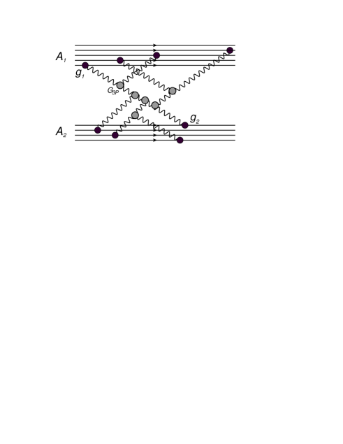
Figure 1: The full set of the diagrams that contribute to the scattering amplitude in the kinematic region Eq. (1.1) or Eq. (2.21).

2 The BFKL Pomeron Calculus

2.1 Main ingredients of the BFKL Pomeron Calculus

The main ingredients of the BFKL Pomeron Calculus are the same as in the Pomeron Calculus in zero transverse dimensions (see Fig. 1), including the Green function of the Pomeron and the vertices of the Pomeron interaction. In the BFKL Pomeron Calculus only the triple Pomeron vertex and the vertex of the Pomeron interaction with the nucleon contribute. The first one can be calculated in perturbative QCD which is discussed later on, while the Pomeron - nucleon vertex is a pure non-perturbative input. However, in order to make all of the calculations more transparent, we will assume the model where the nucleus is a bag of $A$ onia, where each of them consists of a heavy quark and antiquark. The typical distances in the onium are small and of the order of $1/m_{Q}$, where $m_{Q}$ is the heavy quark mass. Therefore, in this oversimplified model we can perform all estimates in the framework of perturbative QCD.

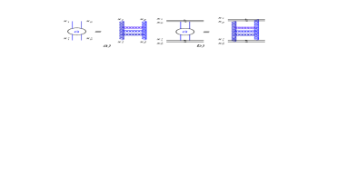
Figure 2: The graphical form of the BFKL Pomeron Green function in the coordinate representation (Fig. 3(a)) and the amplitude for onium-onium scattering (Fig. 3(b)).

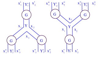
Figure 3: The graphical form of the triple Pomeron vertex in the coordinate representation.

One of the main ingredients of this approach is the Green function of the BFKL Pomeron $G\left(x_{1},x_{2}|x^{\prime}_{1},x^{\prime}_{2}\right)$ (see Fig. 3). The explicit expression for this Green function can be found in Ref.[18]. The onium-onium forward scattering amplitude can be easily written using the Green function in the following form;

$$A\left(Y=lns,t=0\right)\,\,=\,\,\alpha_{S}^{2}\int d^{2}b\int d^{2}r\,\int d^{2}R\,|\Psi\left(r\right)|^{2}\,|\Psi\left(r\right)|^{2}\,G\left(x^{\prime}_{1},x^{\prime}_{2};0|x_{1},x_{2};Y\right)$$ (2.2)

where $\alpha_{S}$ is the QCD coupling , $\Psi$ is the wave function of the onium, $b$ is the impact parameter which is equal to $\vec{b}\,=\,\frac{1}{2}\left(\vec{x}_{1}+\vec{x}_{2}+\vec{x}^{\prime}_{1}+\vec{x}^{\prime}_{2}\right)$ and $\vec{r}=\vec{x}_{1}-\vec{x}_{2}$ and $\vec{R}=\vec{x}^{\prime}_{1}-\vec{x^{\prime}}_{2}$ are the transverse sizes of the two scattering colorless dipoles. The Green function has a simple form in this particular case, namely

$$G\left(r,R;t=0,Y\right)\,\,\equiv\,\,\int d^{2}b\,G\left(x_{1},x_{2};0|x_{1},x_{2};Y\right)\,\,=\,\,\int^{i\epsilon+\infty}_{i\epsilon-\infty}\frac{d\nu}{2\pi}\,\lambda\left(0,\nu\right)\,\frac{1}{\sqrt{r^{2}\,R^{2}}}\,\left(\frac{r^{2}}{R^{2}}\right)^{i\nu}\,e^{\omega(\nu)\,Y}$$ (2.3)

The energy levels $\omega(\nu)$ are the BFKL eigenvalues

$$\omega(\nu)\,=\,2\,\bar{\alpha}_{S}\left(\psi(1)-Re{\,\psi\left(\frac{1}{2}+i\nu\right)}\right)\,\,=\,\,\bar{\alpha}_{S}\left(2\psi(1)-\psi\left(\gamma\right)-\psi\left(1-\gamma\right)\right)\,\,=\,\,\bar{\alpha}_{S}\,\chi\left(\gamma\right)$$ (2.4)

where $\psi(z)=d\ln\Gamma(z)/dz$ and $\Gamma(z)$ is the Euler gamma function, $\gamma=\frac{1}{2}+i\nu$ is the anomalous dimension, and $\bar{\alpha}_{S}=\alpha_{S}N_{c}/\pi$ where $N_{c}$ is the number of colors. Finally

$$\lambda(0,\nu)\,=\frac{1}{[1+4\nu^{2}]^{2}}$$ (2.5)

We do not need to know the explicit expression for the more general case. Instead of this we will discuss some key properties of the more generalized Green function. However before this we give the expression for the triple Pomeron interaction [9] which can be written in the coordinate representation for the following process. Two reggeized gluons with coordinates $x^{\prime}_{1}$ and $x^{\prime}_{2}$ at rapidity $Y^{\prime}_{1}$, which we denote as $\left\{x^{\,\prime}_{1},x^{\,\prime}_{2}|Y^{\,\prime}_{1}\right\}$, decays into two gluon pairs $\left\{x^{\prime\prime}_{1},x^{\prime\prime}_{3}|Y^{\prime}_{2}\right\}$ and $\left\{x^{\prime\prime}_{2},x^{\prime\prime}_{3}|Y^{\prime}_{3}\right\}$ due to the Pomeron splitting at rapidity $Y$. This Pomeron splitting is shown pictorially in Fig. 3.

$$2\frac{\pi\,\bar{\alpha}^{2}_{S}}{N_{c}}\,\int\,\frac{d^{2}x_{1}\,d^{2}\,x_{2}\,d^{2}x_{3}}{x^{2}_{12}\,x^{2}_{23}\,x^{2}_{13}}\,\left(L_{12}\,G(x^{\prime}_{1},x^{\prime}_{2};Y^{\prime}_{1}|x_{1},x_{2};Y)\right)\times$$

$$\times G(x_{1},x_{3};Y|x^{\prime\prime}_{1},x^{\prime\prime}_{3};Y^{\prime}_{2})\,G(x_{3},x_{2};Y|x^{\prime\prime}_{3},x^{\prime\prime}_{2};Y^{\prime}_{3})$$

where $$L_{12}\,\,\,=\,\,x^{4}_{12}\,p^{2}_{1}\,p^{2}_{2}\,\,\,\hskip 14.22636pt\mbox{with}\hskip 14.22636pt\,\,p^{2}\,=\,-\nabla^{2}\,\,\,\hskip 14.22636pt\mbox{and}\hskip 14.22636pt\,\,\,x^{2}_{12}\,\,=\,\,\left(\vec{x}_{1}\,-\,\vec{x}_{2}\right)^{2}\hskip 56.9055pt$$ (2.7)

For further presentation we require some properties of the BFKL Green function, which are listed below [18]:

1. The general definition of the Green function leads to

   $$G^{-1}(x_{1},x_{2};Y|x^{\prime}_{1},x^{\prime}_{2};Y^{\prime})\,\,\,=\,p^{2}_{1}\,p^{2}_{2}\,\left(\frac{\partial}{\partial Y}+H\right)\,\,=\,\,\left(\frac{\partial}{\partial Y}+H^{+}\right)\,p^{2}_{1}\,p^{2}_{2}$$ (2.8)

   $$Hf(x_{1},x_{2};Y)\,\,=\,\,\frac{\bar{\alpha}_{S}}{2\pi}\,\int\,d^{2}x_{3}\,K\left(x_{1},x_{2}|x_{3}\right)\,\left\{f(x_{1},x_{2};Y)\,-\,f(x_{1},x_{3};Y)\,-\,f(x_{3},x_{2};Y)\right\}\hskip 28.45274pt$$ (2.9)

   $$K\left(x_{1},x_{2}|x_{3}\right)\,\,=\,\,\frac{x^{2}_{12}}{x^{2}_{23}\,x^{2}_{13}}$$ (2.10)

2. The initial Green function $G_{0}$ that corresponds to the exchange of two gluons, is equal to

   $$G_{0}(x_{1},x_{2};Y|x^{\prime}_{1},x^{\prime}_{2};Y)\,\,=\,\,\pi^{2}\,\ln\left(\frac{x^{2}_{1,1^{\prime}}\,x^{2}_{2,2^{\prime}}}{x^{2}_{1,2^{\prime}}\,x^{2}_{1^{\prime},2}}\right)\,\ln\left(\frac{x^{2}_{1,1^{\prime}}\,x^{2}_{2,2^{\prime}}}{x^{2}_{1,2}\,x^{2}_{1^{\prime},2^{\prime}}}\right)$$ (2.11)

   This form of $G_{0}$ has been discussed in Ref.[18].

3. It should be stressed that

   $$\nabla^{2}_{1}\,\nabla^{2}_{2}\,G_{0}(x_{1},x_{2};Y|x^{\prime}_{1},x^{\prime}_{2};Y)=$$ (2.12)

   $$=(2\,\pi)^{4}\,\,\left(\delta^{(2)}(x_{1}-x^{\prime}_{1})\,\delta^{(2)}(x_{2}-x^{\prime}_{2})\,+\,\delta^{(2)}(x_{1}-x^{\prime}_{2})\,\delta^{(2)}(x_{2}-x^{\prime}_{1})\,\right)$$

4. At high energy the Green function is also the eigenfunction of the operator $L_{12}$:

   $$L_{12}\,G(x_{1},x_{2};Y|x^{\prime}_{1},x^{\prime}_{2};Y^{\prime})\,\,=\,\,\frac{1}{\lambda(0,\nu)}\,G(x_{1},x_{2};Y|x^{\prime}_{1},x^{\prime}_{2};Y^{\prime})\,\,\approx\,\,G(x_{1},x_{2};Y|x^{\prime}_{1},x^{\prime}_{2};Y^{\prime});$$ (2.13)

The last equation holds only approximately in the region where $\nu\,\ll\,1$, but this is the most interesting region which is responsible for the high energy asymptotic behavior of the scattering amplitude.

2.2 Functional integral formulation of the BFKL Pomeron Calculus.

The theory with the interaction given by Eq. (2.3) and Eq. (2.1) can be written through the functional integral [9]

$$Z[\Phi,\Phi^{+}]\,\,=\,\,\int\,\,D\Phi\,D\Phi^{+}\,e^{S}\,\,\,\hskip 14.22636pt\mbox{with}\hskip 14.22636pt\,S\,=\,S_{0}\,+\,S_{I}\,+\,S_{E}$$ (2.14)

where $S_{0}$ describes free Pomerons, $S_{I}$ corresponds to their mutual interaction while $S_{E}$ relates to the interaction with the external sources (target and projectile). From Eq. (2.1) and Eq. (2.14) it is clear that

$$S_{0}\,=\,\int\,dY\,dY^{\prime}\,d^{2}x_{1}\,d^{2}x_{2}\,d^{2}x^{\prime}_{1}\,d^{2}x^{\prime}_{2}\,\Phi^{+}(x_{1},x_{2};Y)\,G^{-1}(x_{1},x_{2};Y|x^{\prime}_{1},x^{\prime}_{2};Y^{\prime})\,\Phi(x^{\prime}_{1},x^{\prime}_{2};Y^{\prime})$$ (2.15)

$$S_{I}\,=\,\frac{2\,\pi\bar{\alpha}_{S}^{2}}{N_{c}}\,\int\,dY^{\prime}\,\int\,\frac{d^{2}x_{1}\,d^{2}x_{2}\,d^{2}x_{3}}{x^{2}_{12}\,x^{2}_{23}\,x^{2}_{13}}\,\{\left(L_{12}\Phi(x_{1},x_{2};Y^{\prime})\,\right)\,\Phi^{+}(x_{1},x_{3};Y^{\prime})\,\Phi^{+}(x_{3},x_{2};Y^{\prime})\,\,+\,\,h.c.\}$$ (2.16)

For $S_{E}$ we have the local interaction both in terms of rapidity and coordinates, namely

$$S_{E}\,=\,-\,\int\,dY^{\prime}\,d^{2}x_{1}\,d^{2}x_{2}\,\{\Phi(x_{1},x_{2};Y^{\prime})\,\tau_{pr}(x_{1},x_{2};Y)\,\,+\,\,\Phi^{+}(x_{1},x_{2};Y^{\prime})\,\tau_{tar}(x_{1},x_{2};Y)\}$$ (2.17)

where $\tau_{pr}$ ($\tau_{tar}$) stands for the projectile and target, respectively. The form of the functions $\tau$ depend on the non-perturbative input in our problem. In our simple model of the nucleus they have the following form

$$\tau_{pr}\,=\,\,\delta\left(Y-Y^{\prime}\right)\,|\Psi\left(x_{12}\right)|^{2}\,S_{A_{1}}\left(\vec{B}-\vec{b}\right);\,\,\,\,\,\tau_{tar}\,=\,\,\delta\left(Y^{\prime}-0\right)\,|\Psi\left(x_{12}\right)|^{2}\,S_{A_{2}}\left(\vec{b}\right)$$ (2.18)

where $Y=lns$ and $S_{A_{i}}\left(b\right)$ is the number of nucleons at a given impact parameter $b$ in the nucleus $A_{i}$. $\vec{B}$ is the impact parameter between the centers of the two nuclei and $b$ is the position of the interacting nucleon (onium) in the target. In Eq. (2.18) we neglect the impact parameter of the onium - onium interaction in comparison with the impact parameters of the nucleons (onia) in the nuclei. Indeed, the impact parameter of the onium - onium interaction is of the order of the typical onium (nucleon) size, which is much less than the nucleus size. This is a key assumption of the Glauber approach [24] which restricts the value of energy until we can trust this approach. The radius of the onium-onium interaction increases with energy, and at ultra high energy it will be larger than the nucleus size. A discussion of this increase in the framework of QCD can be found in Ref. [25]. This assumption means that we can integrate over all impact parameters in the Pomeron interaction, and actually all fields $\Phi\left(x_{1},x_{2}\right)$ and $\Phi^{+}\left(x_{1},x_{2}\right)$ can be considered to be the fields that depend only on the dipole sizes ($\Phi\left(x_{12}\right)$ and $\Phi^{+}\left(x_{12}\right)$).

2.3 The equation for nucleus-nucleus scattering

Fig. 5 shows the Glauber re-scatterings that give the largest contribution to the nucleus-nucleus scattering amplitude. The onium (nucleon) - onium (nucleon) scattering amplitude is of the order of $\alpha_{S}^{2}$ and the exchange of one BFKL Pomeron leads to the following contribution to the nucleus-nucleus scattering amplitude

$$A_{{I\!\!P}}\left(Y,B\right) = \alpha_{S}^{2}\int d^{2}b\,S_{A_{1}}\left(\vec{B}-\vec{b}\right)\,S_{A_{2}}\left(b\right)\,\int d^{2}r\,d^{2}R\,|\Psi\left(r\right)|^{2}\,|\Psi\left(R\right)|^{2}\,\int d^{2}b^{\prime}\,G\left(R;0|r,b^{\prime};Y\right)\hskip 28.45274pt$$

$$= \alpha_{S}^{2}\!\int d^{2}b\,S_{A_{1}}\left(\vec{B}-\vec{b}\right)\,S_{A_{2}}\left(b\right)\,\int d^{2}r\,|\Psi\left(r\right)|^{2}\,{\cal G}\left(r;Y\right)\,\propto\,\alpha_{S}^{2}\,A^{1/3}_{1}\,A^{1/3}_{2}\,A^{2/3}_{1}\mbox{(for $A_{1}<A_{2}$)}\,e^{\omega(0)\,Y}$$

Notice that the factor $A^{2/3}_{1}$ stems from the $b$ integration. The contribution of the triple Pomeron interaction leads to the amplitude shown in Fig. 5. Using Eq. (2.1) and the function ${\cal G}\left(r;Y\right)$ that has been introduced in Eq. (2.3), this contribution can be rewritten in the form

$$2\bar{\alpha}_{S}\alpha_{S}^{4}\int\!d^{2}b\,S_{A_{1}}\left(\vec{B}-\vec{b}\right)\,S^{2}_{A_{2}}\left(b\right)\int^{Y}_{0}\!\!dY^{\prime}\int\,\frac{d^{2}x_{1}\,d^{2}\,x_{2}\,d^{2}x_{3}}{x^{2}_{12}\,x^{2}_{23}\,x^{2}_{13}}\,L_{12}\,{\cal G}\left(x_{12};Y-Y^{\prime}\right)\,$$ (2.20)

$$\times{\cal G}\left(x_{23};Y^{\prime}-0\right)\,{\cal G}\left(x_{23};Y^{\prime}-0\right)\,\,\,\propto\,\,\,\,\Big{(}\alpha_{S}^{2}\,A^{1/3}_{1}\,A^{1/3}_{2}\,A^{2/3}_{1}\,e^{\omega(0)\,Y}\Big{)}\,\Big{(}\alpha_{S}^{2}A^{1/3}_{2}\,e^{\omega(0)\,Y}\Big{)}$$

$$\,\,\sim\,\,\,\,\,A_{{I\!\!P}}\left(Y,B\right)\Big{(}\alpha_{S}^{2}A^{1/3}_{2}\,e^{\omega(0)\,Y}\Big{)}$$

Eq. (2.20) shows that if

$$\alpha_{S}^{2}\,A^{1/3}_{1}\,A^{1/3}_{2}\,e^{\omega(0)\,Y}\,\,\sim\,\,1;\,\,\,\mbox{but}\,\,\,\,\alpha_{S}^{2}\,A^{1/3}_{1}\,e^{\omega(0)\,Y}\,\,\leq\,\,1$$ (2.21)

the diagrams with triple Pomeron interactions are small and only the Glauber - type re-scatterings shown in Fig. 5, give the largest contribution to the nucleus-nucleus scattering amplitude. However, if

$$\alpha_{S}^{2}\,A^{1/3}_{1}\,e^{\omega(0)\,Y}\,\,\sim\,\,1\,\,\,\mbox{while}\,\,\,\alpha_{S}^{2}\,e^{\omega(0)\,Y}\,\,\leq\,\,1$$ (2.22)

the “net” diagrams of Fig. 1 will also contribute. The set of “net” diagrams (see Fig. 1) has two topological characteristics: (1) these diagrams are two nuclei irreducible or, in other words, any diagram cannot be redrawn as two parts separated by two nuclei states in the $s$-channel; and (2) the smallness of each triple Pomeron vertex ($G_{3{I\!\!P}}\propto\alpha_{S}^{2}$) is compensated by a large factor of $A^{1/3}_{1}$ or $A^{1/3}_{2}$. The smallness of $\alpha_{S}^{2}\,e^{\omega(0)\,Y}$ leads to the fact that we can neglect the BFKL Pomeron loops or corrections to Pomeron vertices which are of the order of $\int dY_{1}dY_{2}G_{3{I\!\!P}}(Y_{1})\,G_{3{I\!\!P}}(Y_{2})\exp\left(\omega(0)(Y_{1}-Y_{2})\right)\propto\alpha_{S}^{2}\exp\left(\omega(0)Y\right)$.

It is obvious that in order to sum both the Glauber re-scatterings and the net diagrams, we need to search for the nucleus-nucleus scattering amplitude in the form

$$A\left(AA;s,B\right)\,\,=\,\,i\Big{(}1\,\,-\,\,\exp\left(-\frac{1}{2}\Omega\left(s,B\right)\right)\Big{)}$$ (2.23)

where $$\Omega\left(s,B\right)\,\,=\,\,A_{{I\!\!P}}\left(Y,B\right)\,\,+\,\,\dots\,=\,\mbox{net diagrams}$$

$$=\alpha_{S}^{2}A^{1/3}_{1}\,A^{1/3}_{2}A^{2/3}_{1}s^{\omega(0)}\Sigma\Big{(}\alpha_{S}^{2}A^{1/3}_{1}\,s^{\omega(0)},\alpha_{S}A^{1/3}_{2}e^{\omega(0)}\Big{)}\hskip 28.45274pt\mbox{(for $A_{1}<A_{2}$)}\,$$

Indeed, the Glauber form of Eq. (2.23) sums all two nuclei reducible diagrams (see Fig. 5 and Fig. 5) while net diagrams, being two nuclei irreducible, provide the contribution $\Omega/2$ (see Fig. 5). The normalization of Eq. (2.23) is the following

$$\sigma_{tot}\left(AA;s\right)\,\,=\,\,2\,\int d^{2}B\,\mbox{Im}A\left(AA;s,B\right)$$ (2.25)

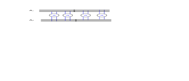
Figure 4: The Glauber-type re-scattering for the nucleus-nucleus scattering amplitude

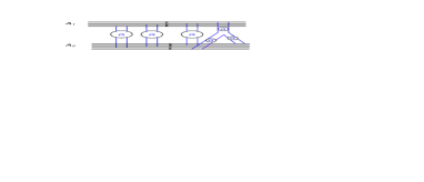
Figure 5: The contribution of the triple Pomeron vertex to the Glauber-type formula.

The equations that sum the net diagrams of Fig. 1 can be derived from [9, 19] from the following equations of motion

$$\frac{\delta S}{\delta\Phi\left(x,y\right)}\,\,=\,\,0;\,\,\,\,\,\,\,\,\frac{\delta S}{\delta\Phi^{+}\left(x,y\right)}\,\,=\,\,0;$$ (2.26)

Using the action of Eq. (2.14), one can derive from Eq. (2.26) the system of two equations of motion for the theory given by Eq. (2.14):

$$\frac{\partial\langle\Phi(x,y;Y^{\prime})\rangle}{\partial\,Y^{\prime}}\,\,=$$ (2.27)

$$\frac{\bar{\alpha}_{S}}{2\pi}\!\int\!d^{2}z\,K\left(x,y|z\right)\Big{\{}\langle\Phi(x,z;Y^{\prime})\rangle+\langle\Phi(z,y;Y^{\prime})\rangle-\langle\Phi(x,y;Y^{\prime})\rangle-4\pi\alpha_{S}\langle\Phi(z,y;Y^{\prime})\Phi(z,y;Y^{\prime})\rangle\Big{\}}$$

$$-\frac{1}{(2\pi)^{4}}\frac{\bar{\alpha}_{S}}{\pi}4\pi\alpha_{S}\int d^{2}z\frac{d^{2}x^{\prime}d^{2}\,y^{\prime}}{(x^{\prime}-y^{\prime})^{4}}G_{0}\left(x,y;Y^{\prime}|x^{\prime},y^{\prime};Y^{\prime}\right)K\left(x^{\prime},y^{\prime}|z\right)\langle\left\{L_{zy^{\prime}}\Phi^{+}\left(z,y^{\prime},Y-Y^{\prime}\right)\right\}\Phi(x^{\prime},z;Y^{\prime})\rangle$$

$$-\frac{\partial\langle\Phi^{+}(x,y;Y-Y^{\prime})}{\partial\,Y^{\prime}}=$$ (2.28)

$$=\frac{\bar{\alpha}_{S}}{2\pi}\,\int\,d^{2}zK\left(x,y|z\right)\Big{\{}\langle\Phi^{+}(x,z;Y-Y^{\prime})\rangle+\langle\Phi^{+}(z,y;Y-Y^{\prime})\rangle-\langle\Phi^{+}(x,y;Y-Y^{\prime})\rangle-\Big{.}$$

$$-\Big{.}4\pi\alpha_{S}\langle\Phi^{+}(z,y;Y-Y^{\prime})\Phi^{+}(z,y;Y-Y^{\prime})\rangle\Big{\}}$$

$$-\frac{1}{(2\pi)^{4}}\frac{\bar{\alpha}_{S}}{\pi}4\pi\alpha_{S}\int d^{2}z\frac{d^{2}x^{\prime}d^{2}y^{\prime}}{(x^{\prime}-y^{\prime})^{4}}G_{0}\left(x,y;Y^{\prime}|x^{\prime},y^{\prime};Y^{\prime}\right)K\left(x^{\prime},y^{\prime}|z\right)\langle\left\{L_{zy^{\prime}}\Phi\left(z,y^{\prime};Y^{\prime}\right)\right\}\Phi^{+}(x^{\prime},z;Y-Y^{\prime})\rangle\,$$

In Eq. (2.27) and Eq. (2.28) the procedure of averaging is defined as

$$\langle O(x,z;Y^{\prime})\rangle\,\,\equiv\,\frac{\int D\Phi D\Phi^{+}\,O(x,z,Y)\,e^{S\left[\Phi,\Phi^{+}\right]}}{\int D\Phi D\Phi^{+}\,\,e^{S\left[\Phi,\Phi^{+}\right]}|_{S_{E}=0}}$$ (2.29)

Eq. (2.27) and Eq. (2.28) are general equations for the theory of interacting BFKL Pomerons which sum all possible diagrams. For the net diagrams we have the additional property that

$$\langle\Phi(x,z;Y)\,\Phi(z,y;Y)\rangle=\langle\Phi(x,z;Y)\rangle\,\langle\Phi(z,y;Y)\rangle;\,\,\,\langle\Phi^{+}(x,z;Y)\,\Phi^{+}(z,y;Y)\rangle=\langle\Phi^{+}(x,z;Y)\rangle\,\langle\Phi^{+}(z,y;Y)\rangle;$$

$$\langle\Phi^{+}(x,z;Y)\,\Phi(z,y;Y)\rangle\,\,=\,\,\langle\Phi^{+}(x,z;Y)\rangle\,\langle\Phi(z,y;Y)\rangle$$ (2.30)

Indeed, drawing all diagrams in the kinematic region of Eq. (2.22) for $\langle\Phi(x,z;Y)\,\Phi(z,y;Y)\rangle$ one can see that we have two sets of diagrams, that are disconnected from each other. Introducing

$$N\left(x,y;Y\right)\,\, = \,\,-4\pi\alpha_{S}\frac{\int D\Phi D\Phi^{+}\,\Phi(x,z,Y)\,e^{S\left[\Phi,\Phi^{+}\right]}}{\int D\Phi D\Phi^{+}\,\,e^{S\left[\Phi,\Phi^{+}\right]}|_{S_{E}=0}}\,\,\,\,\,\,\,\,\mbox{and}$$

$$N^{+}\left(x,y;Y\right)\,\, = \,\,-4\pi\alpha_{S}\frac{\int D\Phi D\Phi^{+}\,\Phi^{+}(x,z,Y)\,e^{S\left[\Phi,\Phi^{+}\right]}}{\int D\Phi D\Phi^{+}\,\,e^{S\left[\Phi,\Phi^{+}\right]}|_{S_{E}=0}}$$ (2.31)

and using Eq. (2.30) we rewrite Eq. (2.27) and Eq. (2.28) in the form

$$\frac{\partial N(x,y;Y^{\prime})}{\partial\,Y^{\prime}}\,\,=$$

$$= \,\,\frac{\bar{\alpha}_{S}}{2\pi}\,\int\,d^{2}\,z\,K\left(x,y|z\right)\,\Big{\{}N(x,z;Y^{\prime})\,+\,N(z,y;Y^{\prime})\,-\,N(x,y;Y^{\prime})\,-N(z,y;Y^{\prime})\,N(z,y;Y^{\prime})\Big{\}}$$

$$- \,\frac{1}{(2\pi)^{4}}\,\frac{\bar{\alpha}_{S}}{\pi}\,\int d^{2}z\,\frac{d^{2}x^{\prime}\,d^{2}\,y^{\prime}}{(x^{\prime}-y^{\prime})^{4}}\,G_{0}\left(x,y;Y^{\prime}|x^{\prime},y^{\prime};Y^{\prime}\right)\,\,K\left(x^{\prime},y^{\prime}|z\right)\,\,\left\{L_{zy^{\prime}}\,N^{+}\left(z,y^{\prime},Y-Y^{\prime}\right)\right\}\,N(x^{\prime},z;Y^{\prime})\,$$

$$-\,\frac{\partial N^{+}(x,y;Y-Y^{\prime})}{\partial\,Y^{\prime}}\,\,=\,\,$$

$$= \,\,\frac{\bar{\alpha}_{S}}{2\pi}\,\int\,d^{2}\,z\,K\left(x,y|z\right)\,\Big{\{}N^{+}(x,z;Y-Y^{\prime})\,+\,N^{+}(z,y;Y-Y^{\prime})\,-\,N^{+}(x,y;Y-Y^{\prime})\,-\Big{.}$$

$$- \Big{.}\,\,N^{+}(z,y;Y-Y^{\prime})\,N^{+}(z,y;Y-Y^{\prime})\Big{\}}$$

$$- \,\,\frac{1}{(2\pi)^{4}}\,\frac{\bar{\alpha}_{S}}{\pi}\,\int d^{2}z\frac{d^{2}x^{\prime}\,d^{2}\,y^{\prime}}{(x^{\prime}-y^{\prime})^{4}}\,G_{0}\left(x,y;Y^{\prime}|x^{\prime},y^{\prime};Y^{\prime}\right)\,\,K\left(x^{\prime},y^{\prime}|z\right)\,\left\{L_{zy^{\prime}}N\left(z,y^{\prime};Y^{\prime}\right)\right\}\,N^{+}(x^{\prime},z;Y-Y^{\prime})\,$$

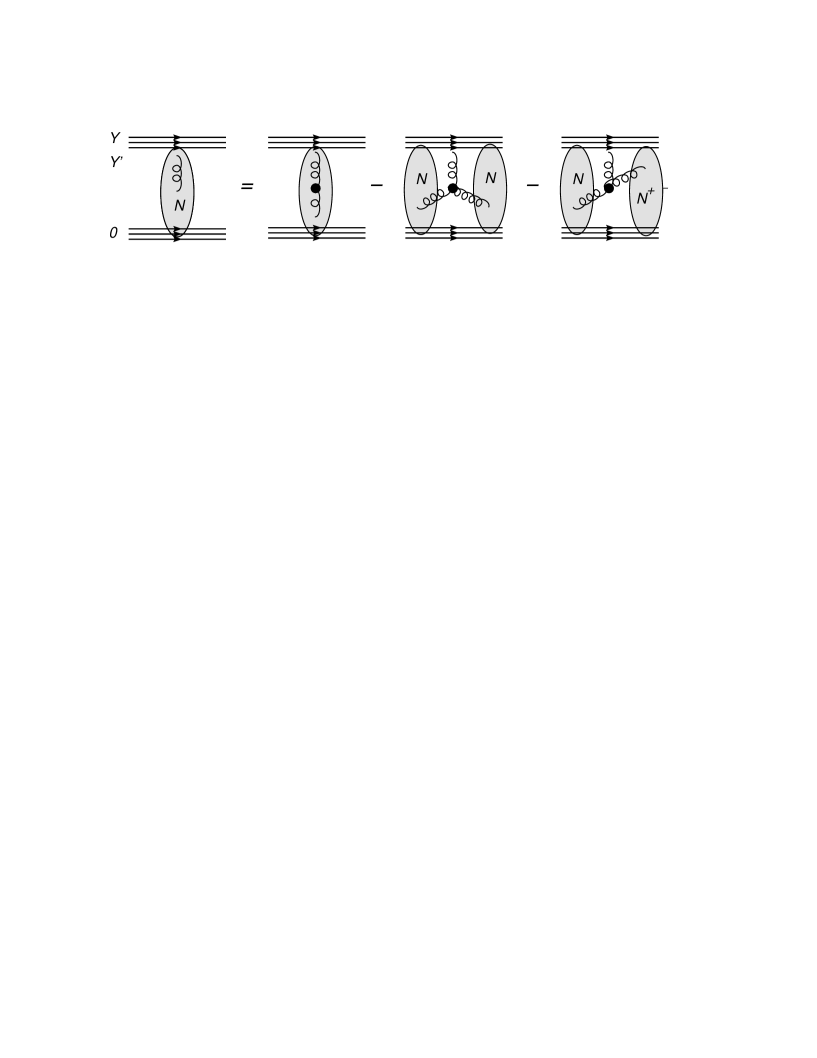
Figure 6: The pictorial representation of Eq. (2.3) )(see Fig. 6-A). Fig. 6-B shows the initial condition for this equation. The black blob denotes the triple gluon vertex while the wavy lines describe BFKL Pomerons.

Figure 7: The diagrams for $N$. In Fig. 7-A we denote by bold wavy lines and by normal lines, the Pomerons that contribute to the different $N$ and $N^{2}$ terms of Eq. (2.3) (see Fig. 6-A). In Fig. 7-B the Pomeron that connects the two sets of diagrams is shown in blue. One can see that its contribution is suppressed by a factor of $\alpha_{S}^{2}s^{\omega(0)}$.

The graphical form of the first equation (Eq. (2.3)) is shown in Fig. 6-A. The equation for $N^{+}$ has the same graphical form with the replacement $N\to N^{+}$ and $N^{+}\to N$. Note, that the initial condition for $N^{+}$ has the form of Fig. 6-B but with the Pomeron attached to the upper nucleus.

Using the initial condition of Fig. 6-B one can check that the iterations of Eq. (2.3) reproduce the set of net diagrams of Fig. 1. Comparing Fig. 1 with Fig. 6 one can see that Eq. (2.3) sums the net diagrams, proving that the set of equations of Eq. (2.3) and Eq. (2.3) describe the nucleus-nucleus scattering. Eq. (2.30) leads to the second and the third terms of equation. These terms reflect the key property of the net diagrams, namely that three Pomerons in a triple Pomeron vertex generates the two sets of diagrams that are disconnected from each other (see Fig. 7-A, where these two sets of diagrams are shown in bold and normal wavy lines). In other words, each Pomeron line that connects two sets of diagrams gives the contribution of the order of $\alpha_{S}^{2}\,e^{\omega(0)\,Y}\,\,\leq\,\,1$ (see Fig. 7-B for example).

By assuming that $N^{+}$ is small, Eq. (2.3) reduces to the familiar Balitsky-Kovchegov (BK) equation.

The typical example of this type of situation is deep inelastic scattering (DIS), but even in this case we have to be careful [26]. Indeed, the BK equation sums the class of “fan” diagrams shown in Fig. 9. For large photon virtualities $Q$, it is sufficient to take into account just the scattering of one dipole whose transverse size is of the order of $1/Q$. However, the typical sizes of the dipoles inside of the diagrams of Fig. 9 can reach values, such that it is no longer justified to use this class of “fan” diagrams [1, 26].

It is interesting to notice that in the B-K limit, $N$ being the Green function of two gluons can be viewed as the amplitude of the dipole scattering. In the case of nucleus-nucleus scattering the scattering amplitude of a dipole that interacts with two nuclei is a more complicated observable which for small $N$ and $N^{+}$ is equal to $N+N^{+}$.

It should be stressed that the proof of Eq. (2.3) and Eq. (2.3), as well as the relation to BFKL Pomeron diagrams were discussed in Refs.[9, 19, 20, 21] as well as in Ref.[22] for the BFKL Pomeron Calculus in zero transverse dimensions. In this section we just introduce notations and the main ingredients of this approach for completeness of presentation.

Figure 8: The “fan” diagrams that are summed by the Balitsky-Kovchegov equation. The zig zag lines denote the BFKL Pomeron.

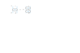
Figure 9: The graphical form of the BFKL contribution of Eq. (3.34).

3 Solution to the main equations deeply in the saturation region.

3.1 Two saturation scales.

In Ref.[26], it is shown that actually we are dealing with two saturation scales even in the dilute-dense scattering system. Indeed, let us consider the BFKL Pomeron contribution to the case of DIS. From the complete set of eigenfunctions of the BFKL equation, one can conclude that (see Eq. (2.3))

$$G\left(r,R;t=0,Y\right)\,\,=\,\,\int\,d^{2}r^{\prime}\,G\left(r,r^{\prime};t=0,Y-Y^{\prime}\right)\,G\left(r^{\prime},R;t=0,Y^{\prime}-0\right)\,$$ (3.34)

$$=\,\,\frac{1}{\sqrt{r^{2}R^{2}}}\int^{i\epsilon+\infty}_{i\epsilon-\infty}\frac{d\nu^{\prime}}{2\pi}\int^{i\epsilon+\infty}_{i\epsilon-\infty}\frac{d\nu}{2\pi}\int\frac{d^{2}r^{\prime}}{r^{\prime 2}}\,\left(\frac{r^{2}}{r^{\prime 2}}\right)^{i\nu}\,\left(\frac{r^{\prime 2}}{R^{2}}\right)^{i\nu^{\prime}}\exp\Big{\{}\omega(\nu)(Y-Y^{\prime})\,+\,\omega(\nu^{\prime})(Y^{\prime}-0)\Big{\}}$$

Integrating over $r^{\prime}$ leads to $\delta(\nu-\nu^{\prime})$ and provides the relation given in Eq. (3.34), which is the general property of the Green function. On the other hand, each of the Green functions in Eq. (3.34) has its own saturation momentum. It is well known [1, 27, 28, 29] that the equation for the saturation scale does not depend on the non-linear terms and can be derived from the knowledge of only the linear part of the equation with the BFKL kernel. Using the general equation for the saturation scale [1, 27, 28, 29], one finds two saturation scales for the two Green functions

$$G\left(r,r^{\prime};t=0,Y-Y^{\prime}\right)\, \,\,\,\rightarrow\,\,\, \,\,\ln\left(r^{2}/r^{\prime 2}_{s}\right)\,\,=\,\,-\frac{\omega\left(\gamma_{cr}\right)}{1-\gamma_{cr}}\,\left(Y\,-\,Y^{\prime}\right);$$ (3.35)

$$G\left(r^{\prime},R;t=0,Y^{\prime}-0\right)\, \rightarrow \,\,\ln\left(r^{\prime 2}_{s}/R^{2}\right)\,\,=\,\,-\frac{\omega\left(\gamma_{cr}\right)}{1-\gamma_{cr}}\,\left(Y\,-\,0\right);$$ (3.36)

where $Q^{2}_{s}\,=\,1/r^{2}_{s}$ and $\gamma=\frac{1}{2}+i\nu$ while $\gamma_{cr}$ can be found from the equation

$$-\,\frac{d\omega\left(\gamma\right)}{d\gamma}|_{\gamma=\gamma_{cr}}\,\,=\,\,\frac{\omega\left(\gamma_{cr}\right)}{1\,-\,\gamma_{cr}}$$ (3.37)

resolving these equations we obtain two saturation scales:

$$\ln\left(Q^{2}_{1,s}\,r^{2}\right)\, = \,-\frac{\omega\left(\gamma_{cr}\right)}{1-\gamma_{cr}}\,\left(Y\,-\,Y^{\prime}\right);$$ (3.38)

$$\ln\left(Q^{2}_{2,s}\,R^{2}\right)\, = \,\,\frac{\omega\left(\gamma_{cr}\right)}{1-\gamma_{cr}}\,\left(Y^{\prime}-0\right);$$ (3.39)

Eq. (3.38) and Eq. (3.39) can be rewritten in the form

$$Q^{2}_{1,s}\, = \,Q^{2}\exp\Big{(}-\frac{\omega\left(\gamma_{cr}\right)}{1-\gamma_{cr}}\,\left(Y\,-\,Y^{\prime}\right)\Big{)};$$ (3.40)

$$Q^{2}_{2,s}\, = \,\,Q^{2}_{2,s}\left(Y=0\right)\,\exp\Big{(}\frac{\omega\left(\gamma_{cr}\right)}{1-\gamma_{cr}}\,\left(Y^{\prime}-0\right)\Big{)};$$ (3.41)

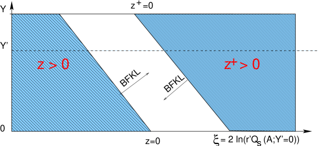
Figure 10: Two saturation scales for DIS.

It is useful to introduce two scaling variables:

$$z^{+}\,\,=\,\,\ln\left(r^{\prime 2}\,Q^{2}_{2,s}\right)\,\,=\,\,\lambda_{s}\,Y^{\prime}+\,\xi;\,\,\,\,\,z\,=\,-\ln\left(r^{\prime 2}\,Q^{2}_{1,s}\right)\,\,=\,\,\lambda_{s}\,\left(Y-Y^{\prime}\right)-\xi$$ (3.42)

where $\xi\,=\,\ln\left(r^{\prime 2}\,Q^{2}_{2,s}(Y^{\prime}=0)\right)$ and $\lambda_{s}=\omega\left(\gamma_{cr}\right)/(1-\gamma_{cr})$. The saturation effects start to be essential when both $z$ and $z^{+}$ are positive. For negative $z$ and $z^{+}$ we can safely use the linear (BFKL) evolution equation (see Fig. 10). For DIS due to the large value of the photon virtuality, we have the region where the size of the dipole is smaller than both of the inverse saturation scales [26, 30] (see Fig. 10). However, in the case of nucleus-nucleus scattering the situation is quite different. In this case in the entire kinematic region of low $x$ we cannot neglect the saturation effects, rather we have to solve the non-linear equations (see Fig. 11). It is worth mentioning that

$$z\,\,+\,\,z^{+}\,\,=\,\,\ln\left(r^{2}Q^{2}_{s}\left(Y\right)\right)\,\,\equiv\,\,\zeta\,\,\,\,\,\,\,\mbox{where}\,\,\,Q^{2}_{s}\,\,=\,\,Q^{2}_{2,s}\left(Y=0\right)e^{\lambda_{s}Y}$$ (3.43)

One recognizes that $Q_{s}$ is the saturation momentum in the Balitsky-Kovchegov equation for DIS. Although the idea of two saturation scales has been on the market during the past six years starting with the paper of Mueller and Shoshi[26], it still needs some demystifying. For this purpose let us consider deep inelastic scattering at low $x$ in the double log approximation (DLA). The main contribution stems from the kinematic region where

$$1\,\gg\,x_{1}\,\gg\,\dots\,\gg\,x_{i}\,\gg\,\dots\,\gg\,x;\,\,\,\,Q_{0}\,\ll\,k_{1,\perp}\,\ll\,\dots\,k_{i,\perp}\,\ll\,\dots\,\ll\,k_{n,\perp}\,\ll\,Q;$$ (3.44)

The dipole amplitude in the momentum representation in the DLA looks as follows

$$N\left(Q;Q_{0};Y\right)\,\,=\,\,Const\frac{Q^{2}_{0}}{Q^{2}}\,\exp\Big{(}2\sqrt{\bar{\alpha}_{S}Y\,\ln\left(Q^{2}/Q^{2}_{0}\right)}\Big{)}$$ (3.45)

and this amplitude satisfies the unitarity constraints $N<1$ if

$$Q^{2}\,>\,Q^{2}_{s}\,\,=\,\,Q^{2}_{0}\,e^{4\bar{\alpha}_{S}Y}$$ (3.46)

Eq. (3.34) can be written in the form

$$N\left(Q;Q_{0};Y\right)\,\,\propto\,\,\int d\ln\left(k^{2}_{i,\perp}/Q^{2}_{0}\right)\,N\left(Q,k_{i,\perp};Y-Y^{\prime}\right)\,N\left(k_{i,\perp},Q_{0};Y^{\prime}\right)$$ (3.47)

The amplitude $N\left(k_{i,\perp},Q_{0};Y^{\prime}\right)\,<\,1$ for

$$k^{2}_{i,\perp}\,>\,Q^{2}_{s}\,=\,Q^{2}_{0}\,e^{4\bar{\alpha}_{S}\,Y^{\prime}}$$ (3.48)

while the amplitude $N\left(Q,k_{i,\perp};Y-Y^{\prime}\right)\,<\,1$ if

$$Q^{2}\,>\,k^{2}_{i,\perp}\,e^{4\bar{\alpha}_{S}(Y-Y^{\prime})}$$ (3.49)

One can see that the value of $k_{i,\perp}$ for which both amplitudes are in the region where we can apply perturbative QCD or, in other words, where both amplitudes are small, has to satisfy the following inequality

$$Q^{2}_{1,s}\,=\,Q^{2}\,e^{-\,4\bar{\alpha}_{S}\,(Y-Y^{\prime})}\,\,>\,\,k^{2}_{i,\perp}\,\,>\,\,Q^{2}_{2,s}\,=\,\,Q^{2}_{0}\,e^{4\bar{\alpha}_{S}\,Y^{\prime}}$$ (3.50)

It should be stressed that even when $Q^{2}$ is large ($Q^{2}>Q^{2}_{s}$, see Eq. (3.46)) and the solution of Eq. (3.45) turns out to be small enough to satisfy the unitarity constraints, the partons inside the DGLAP cascade with transverse momenta given in Eq. (3.50), violate unitarity. If $Q^{2}=Q^{2}_{s}$ (see Eq. (3.46)) both parts of the inequality of Eq. (3.50) are equal and all partons violate unitarity. For $Q^{2}<Q^{2}_{s}$ we have the situation shown in Fig. 11. We hope that this equation clarified the appearance of two saturation scales and explains Fig. 10 and Fig. 11.
It should be stressed that Eq. (3.35) as well as the entire discussion in this section, including Fig. 10 and Fig. 11, are related to the partons (dipoles) that give the main contribution to the total cross section (BFKL Pomeron). To illustrate this point, it is instructive to consider partons with $k_{i,\perp}>>Q$ and $k_{i,\perp}>>Q_{0}$, for which we expect that saturation effects will be small, which would seem to disagree with Eq. (3.50) . These partons do not contribute to the deep inelastic scattering in the DLA approach, as we have seen in Eq. (3.44), and therefore, we do not consider them. However, it is worthwhile to discuss why and how these parton are not essential. For these partons that we are discussing, Eq. (3.34) looks like Eq. (3.47), however

$$N\left(Q;k^{2}_{i,\perp},Y-Y^{\prime}\right)\,\,=\,\,Const\frac{Q^{2}}{k^{2}_{i,\perp}}\,\exp\Big{(}2\,\sqrt{\bar{\alpha}_{S}(Y\,-\,Y^{\prime})\,\ln\left(k^{2}_{i,\perp}/Q^{2}\right)}\,\Big{)}$$ (3.51)

Taking Eq. (3.51) into account, we can rewrite Eq. (3.34) for these partons as

$$N\left(Q;Q_{0};Y\right)\!\!\propto\!\!\int\frac{Q^{2}\,d\ln\left(k^{2}_{i,\perp}/Q^{2}_{0}\right)}{k^{2}_{i,\perp}}\,\exp\Big{(}2\,\sqrt{\bar{\alpha}_{S}(Y\,-\,Y^{\prime})\,\ln\left(k^{2}_{i,\perp}/Q^{2}\right)}+2\,\sqrt{\bar{\alpha}_{S}\,Y^{\prime}\,\ln\left(k^{2}_{i,\perp}/Q^{2}_{0}\right)}\,\Big{)}\hskip 28.45274pt$$ (3.52)

Integration over $k_{i,\perp}$ in Eq. (3.52) leads to $k_{i,\perp}\to Q$, and hence the resulting contribution to $N\left(Q;Q_{0};Y\right)$ is proportional to $\exp\Big{(}2\sqrt{\bar{\alpha}_{S}Y^{\prime}\,\ln\left(Q^{2}/Q^{2}_{0}\right)}\Big{)}\,\ll\,\exp\Big{(}2\sqrt{\bar{\alpha}_{S}Y\,\ln\left(Q^{2}/Q^{2}_{0}\right)}\Big{)}(\mbox{{Eq.~{}(\ref{TS8})}})$. In the general case of Eq. (3.34), the integration measure changes from $d^{2}r^{\prime}/r^{\prime 2}$, to $d^{2}r^{\prime}/\sqrt{r^{2}\,R^{2}}$. Consequently the integration over $r^{\,\prime}$ leads to $\delta\left(\nu-\nu^{\prime}\,-\,i\right)$ instead of $\delta\left(\nu-\nu^{\prime}\right)$. Thus the $\nu^{\prime}$ integration leads to the contribution of such partons that forms a negligible part of the total cross section. It should be mentioned that a much more detailed analysis can be found in Ref.[26]. The last item that we wish to mention, is that we are discussing the total cross section, whereas the contribution to the inclusive cross section has a completely different form, with two saturation momenta, which are different.

3.2 Solution deeply in the saturation region : linearized equations

One can see that in the kinematic region where (see Fig. 11) $z>0$ and $z^{+}>0$, then both amplitudes $N\left(r,R_{0};Y^{\prime}\right)$ and $N^{+}\left(R,r;Y-Y^{\prime}\right)$ are deeply in the saturation region. We can find the solution to Eq. (2.3) and Eq. (2.3) in this region, using experience of solving the Balitsky-Kovchegov equation [31]. In this approach $N$ is replaced with $N=1+\Delta N$ (and similarly for $N^{+}$). This, together with the observation that constant $N^{+}$ in Eq. (2.3), and constant $N$ in Eq. (2.3) don’t contribute, we see that the asymptotic solution is $N=1$. Replacing $N$ with $1+\Delta N$ in Eq. (2.3) and acting with $L_{xy}$ on both sides, and using Eq. (2.12) leads to;

$$\frac{\partial\left(L_{xy}\Delta N(x,y;Y^{\prime})\right)}{\partial\,Y^{\prime}}\,\,=$$ (3.53)

$$\,\,-\frac{\bar{\alpha}_{S}}{2\pi}\,\int\,d^{2}\,z\,K\left(x,y|z\right)\,\left(L_{xy}\Delta N(x,y;Y^{\prime})\right)\,\,-\,\,\frac{\bar{\alpha}_{S}}{\pi}\,\int\,d^{2}\,z\,K\left(x,y|z\right)\left(L_{xz}\Delta N^{+}(x,z;Y^{\prime})\right)$$

In Eq. (3.53) we neglect all contributions of the order $(\Delta N)^{2}$, $\Delta N\,\Delta N^{+}$ and $(\Delta N^{+})^{2}$. A similar result is found by using the analogous above mentioned approach on Eq. (2.3).

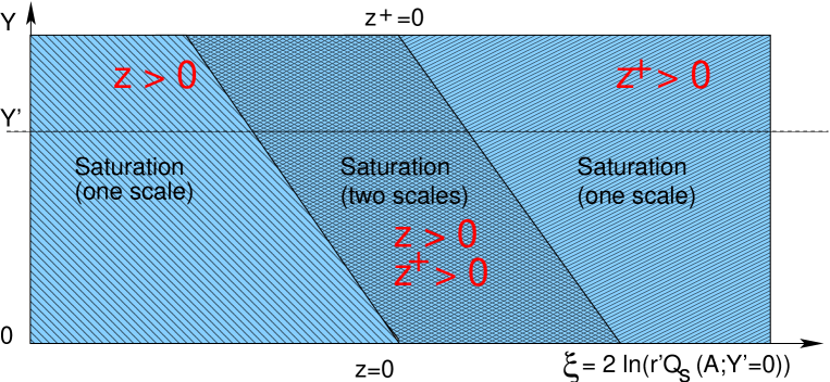
Figure 11: Two saturation scales for nucleus-nucleus scattering.

Introducing the new functions $\tilde{n}=L_{xy}\Delta N$ and $\tilde{n}^{+}\,=\,L_{xy}\Delta N^{+}$ we see that Eq. (2.3) and Eq. (2.3) reduce to two linear equations

$$\frac{\partial\tilde{n}\left(x,y,Y^{\prime}\right)}{\partial\,Y^{\prime}}\,\, = \,\,\,\,-\frac{\bar{\alpha}_{S}}{2\pi}\,\int\,d^{2}\,z\,K\left(x,y|z\right)\,\tilde{n}\left(x,y,Y^{\prime}\right)\,\,-\,\,\frac{\bar{\alpha}_{S}}{\pi}\,\int\,d^{2}\,z\,K\left(x,y|z\right)\tilde{n}^{+}\left(z,y,Y^{\prime}\right)\,\hskip 28.45274pt$$ (3.54)

$$-\,\frac{\partial\tilde{n}^{+}\left(x,y,Y^{\prime}\right)}{\partial\,Y^{\prime}}\,\, = \,\,\,\,-\frac{\bar{\alpha}_{S}}{2\pi}\,\int\,d^{2}\,z\,K\left(x,y|z\right)\,\tilde{n}^{+}\left(x,y,Y^{\prime}\right)\,\,-\,\,\frac{\bar{\alpha}_{S}}{\pi}\,\int\,d^{2}\,z\,K\left(x,y|z\right)\tilde{n}\left(z,y,Y^{\prime}\right)\,\hskip 28.45274pt$$ (3.55)

We first rewrite these equations in a more convenient form:

$$\frac{\partial\tilde{n}\left(x,y,Y^{\prime}\right)}{\partial\,Y^{\prime}}= -\,\,\frac{\bar{\alpha}_{S}}{2\pi}\,\int\,d^{2}\,z\,K\left(x,y|z\right)\,\tilde{n}\left(x,y,Y^{\prime}\right)\,\,-\,\,\frac{\bar{\alpha}_{S}}{2\pi}\,\int\,d^{2}\,z\,K\left(x,y|z\right)\,\tilde{n}^{+}\left(x,y,Y^{\prime}\right)\hskip 28.45274pt$$

$$-\frac{\bar{\alpha}_{S}}{2\pi}\,\int\,d^{2}\,z\,K\left(x,y|z\right)\,\Big{\{}2\tilde{n}^{+}\left(x,z,Y^{\prime}\right)\,\,-\,\,\tilde{n}^{+}\left(x,y,Y^{\prime}\right)\Big{\}}$$

$$-\,\,\frac{\partial\tilde{n}^{+}\left(x,y,Y^{\prime}\right)}{\partial\,Y^{\prime}}= -\,\,\frac{\bar{\alpha}_{S}}{2\pi}\,\int\,d^{2}\,z\,K\left(x,y|z\right)\,\tilde{n}^{+}\left(x,y,Y^{\prime}\right)\,\,-\,\,\frac{\bar{\alpha}_{S}}{2\pi}\,\int\,d^{2}\,z\,K\left(x,y|z\right)\,\tilde{n}\left(x,y,Y^{\prime}\right)\hskip 28.45274pt$$

$$-\frac{\bar{\alpha}_{S}}{2\pi}\,\int\,d^{2}\,z\,K\left(x,y|z\right)\,\Big{\{}2\tilde{n}\left(x,z,Y^{\prime}\right)\,\,-\,\,\tilde{n}\left(x,y,Y^{\prime}\right)\Big{\}}$$

We calculate $\int d^{z}K\left(x,y|z\right)$ taking into account that the main contribution in the saturation region stems from the decay of the large size dipole into one small size dipole and one large size dipole. Indeed,

$$\int d^{2}z\,K\left(x_{1},x_{2}|z\right)\,\,\rightarrow\,\pi\,\int\frac{x^{2}_{12}dx_{13}^{2}}{x^{2}_{13}\,|x^{2}_{12}-x^{2}_{13}|}\,\,=\,\,\pi\int^{x^{2}_{12}}_{\rho^{2}}\frac{dx^{2}_{13}}{x^{2}_{13}}\,\,+\,\,\pi\int^{x^{2}_{12}}_{\rho^{2}}\frac{d|x^{2}_{12}-x^{2}_{13}|}{|x^{2}_{12}-x^{2}_{13}|}$$ (3.58)

$$=\,\,2\pi\ln\left(x^{2}_{12}/\rho^{2}\right)\,\,=\,\,2\pi\,\xi$$

It should be noted that the $\xi$ which is defined in Eq. (3.58), is different from the $\xi$ that appears in Fig. 10 and Fig. 11. At this stage we have introduced the artificial cutoff at small values of the dipole size ($\rho$), but the physical cutoff is $\rho=1/Q_{s}$, as discussed in Ref.[31]. It should be noticed that for the opposite case, when a dipole decays to two dipoles of larger sizes, there is no logarithmic contribution, since

$$\int d^{2}z\,K\left(x_{1},x_{2}|z\right)\,\,\rightarrow\,\pi\,\int^{1/Q^{2}_{s}}_{x^{2}_{12}}\frac{dx^{2}_{13}}{x^{\prime 4}_{13}}\,\,$$ (3.59)

In the two scale kinematic region, the size of the dipole is restricted as follows (see Fig. 11 and Eq. (3.40) and Eq. (3.41));

$$1/Q^{2}_{1,s}\,\,\,\geq\,\,\,r^{\prime 2}\,\,\,\geq\,\,\,1/Q^{2}_{2,s}$$ (3.60)

Therefore, the natural choice is $\rho^{2}=1/Q^{2}_{2,s}$. Using Eq. (3.58), then Eq. (3.2) and Eq. (3.2) simplify to the following;

$$\frac{\partial\tilde{n}\left(x,y,Y^{\prime}\right)}{\partial\,Y^{\prime}}\,\,= \,\,-\bar{\alpha}_{S}\,z^{+}\,\Big{\{}\tilde{n}\left(x,y,Y^{\prime}\right)\,+\,\tilde{n}^{+}\left(x,y,Y^{\prime}\right)\Big{\}}$$

$$-\,\,\frac{\bar{\alpha}_{S}}{2\pi}\,\int\,d^{2}z\,K\left(x,y|z\right)\,\Big{\{}2\tilde{n}^{+}\left(x,z,Y^{\prime}\right)\,\,-\,\,\tilde{n}^{+}\left(x,y,Y^{\prime}\right)\Big{\}}\,$$

$$-\,\frac{\partial\tilde{n}^{+}\left(x,y,Y^{\prime}\right)}{\partial\,Y^{\prime}}\,\,= \,\,-\bar{\alpha}_{S}\,z^{+}\,\Big{\{}\tilde{n}\left(x,y,Y^{\prime}\right)\,+\,\tilde{n^{+}}\left(x,y,Y^{\prime}\right)\Big{\}}$$

$$-\,\,\frac{\bar{\alpha}_{S}}{2\pi}\,\int\,d^{2}z\,K\left(x,y|z\right)\,\Big{\{}2\tilde{n}\left(x,z,Y^{\prime}\right)\,\,-\,\,\tilde{n}\left(x,y,Y^{\prime}\right)\Big{\}}\,$$

We use the double Mellin transform to solve Eq. (3.2) and Eq. (3.2), namely

$$\tilde{n}\left(z^{+},Y^{\prime}\right)\,\,\, =\,\,\int^{\epsilon+i\infty}_{\epsilon-i\infty}\,\frac{d\omega}{2\pi i}\int^{\epsilon+i\infty}_{\epsilon-i\infty}\,\frac{d\gamma}{2\pi i}\,\,\tilde{n}\left(\omega,\gamma\right)\,e^{\omega Y^{\prime}+(1-\gamma)\,z^{+}}$$ (3.63)

$$\tilde{n}^{+}\left(z,Y^{\prime}\right)\,\,\, =\,\,\int^{\epsilon+i\infty}_{\epsilon-i\infty}\,\frac{d\omega}{2\pi i}\int^{\epsilon+i\infty}_{\epsilon-i\infty}\,\frac{d\gamma}{2\pi i}\,\,\tilde{n}^{+}\left(\omega,\gamma\right)\,e^{\omega Y^{\prime}+(1-\gamma)\,z^{+}}$$ (3.64)

Substituting Eq. (3.63) and Eq. (3.64) into Eq. (3.2) and Eq. (3.2), adding and subtracting these two equations we obtain for $\Sigma\Big{(}\omega,\gamma\Big{)}\,=\,\tilde{n}\left(\omega,\gamma\right)\,+\,\tilde{n}^{+}\left(\omega,\gamma\right)$ and $\Delta\Big{(}\omega,\gamma\Big{)}\,=\,\tilde{n}\left(\omega,\gamma\right)\,-\,\tilde{n}^{+}\left(\omega,\gamma\right)$ the following;

$$\left(\omega+\lambda_{s}(1-\gamma)\right)\,\Delta\left(\omega,\gamma\right)\,\,=\,\,-\,2\,\bar{\alpha}_{S}\,\frac{\partial\Sigma\left(\omega,\gamma\right)}{\partial\gamma}\,\,-\,\,\omega\left(\gamma\right)\Sigma\left(\omega,\gamma\right)$$ (3.65)

$$\left(\omega+\lambda_{s}(1-\gamma)\right)\,\Sigma\left(\omega,\gamma\right)\,\,=\,\,\omega\left(\gamma\right)\Delta\left(\omega,\gamma\right);$$ (3.66)

where $\omega\left(\gamma\right)$ is given by Eq. (2.4). Solving Eq. (3.65) we find

$$\Sigma\left(\omega,\gamma\right)\,\, =\,\,\Sigma_{0}\left(\gamma\right)\,\exp\Big{\{}-\,\int^{\gamma}_{0}\,d\gamma^{\,\prime}\,\frac{\Big{(}\omega+\lambda_{s}(1-\gamma^{\,\prime})\Big{)}^{2}+\omega^{2}\left(\gamma^{\,\prime}\right)}{2\bar{\alpha}_{S}\,\omega\left(\gamma^{\,\prime}\right)}\Big{\}}$$ (3.68)

$$=\,\,\Sigma_{0}\left(\gamma\right)\,\exp\Big{\{}\,L\left(\gamma\right)\omega^{2}+F\left(\gamma\right)\omega+K\left(\gamma\right)\Big{\}}$$

where we define

$$L\left(\gamma\right) =-\frac{1}{2\bar{\alpha}_{S}}\int^{\gamma}_{0}\frac{d\gamma^{\,\prime}}{\omega\left(\gamma^{\,\prime}\right)}$$ (3.69)

$$F\left(\gamma\right) =-\frac{1}{\bar{\alpha}_{S}}\int^{\gamma}_{0}d\gamma^{\,\prime}\frac{\lambda_{s}\left(1-\gamma^{\,\prime}\right)}{\omega\left(\gamma^{\,\prime}\right)}$$ (3.70)

$$K\left(\gamma\right) =-\frac{1}{2\bar{\alpha}_{S}}\int^{\gamma}_{0}d\gamma^{\,\prime}\frac{\lambda_{s}^{2}\left(1-\gamma^{\,\prime}\right)^{2}}{\omega\left(\gamma^{\,\prime}\right)}-\frac{1}{2\bar{\alpha}_{S}}\int^{\gamma}_{0}d\gamma^{\,\prime}\omega\left(\gamma^{\,\prime}\right)$$ (3.71)

and where $\Sigma_{0}\left(\gamma\right)$ has to be found from the matching with the regions with one saturation scale (see Fig. 11). Using Eq. (3.68) we obtain the solution in the form

$$\Sigma\left(z^{+},Y^{\prime}\right)\,\,\, =\,\,\int^{\epsilon+i\infty}_{\epsilon-i\infty}\,\frac{d\omega}{2\pi i}\int^{\epsilon+i\infty}_{\epsilon-i\infty}\,\frac{d\gamma}{2\pi i}\,\,\Sigma_{0}\left(\gamma\right)\,e^{\Psi\left(\omega,\gamma,Y^{\prime},z^{+}\right)}$$ (3.72)

$$\Psi\left(\omega,\gamma,Y^{\prime},z^{+}\right)\,\, =\,\,\omega\left(Y^{\,\prime}+F\left(\gamma\right)\right)\,+\,(1-\gamma)\,z^{+}+\omega^{2}L\left(\gamma\right)$$ (3.73)

where the function $K\left(\gamma\right)$ which appears in the exponential function in Eq. (3.68) has been absorbed into the function $\Sigma_{0}\left(\gamma\right)$ in Eq. (3.72). The integral over $\omega$ in Eq. (3.72) can be taken explicitly leading to the following expression

$$\Sigma\left(z^{+},Y^{\prime}\right)\,\,\, =\,-\,\int^{\epsilon+i\infty}_{\epsilon-i\infty}\,\frac{d\gamma}{2\pi i}\,\,\Sigma_{0}\left(\gamma\right)\,\sqrt{\frac{\pi}{L\left(\gamma\right)}}\,\exp\Big{(}\,(1-\gamma)\,z^{+}\,-\frac{\left(Y^{\prime}+F\left(\gamma\right)\right)^{2}}{4L\left(\gamma\right)}\Big{)}$$ (3.75)

$$=\,-\,\int^{\epsilon+i\infty}_{\epsilon-i\infty}\,\frac{d\gamma}{2\pi i}\,\,\tilde{\Sigma}_{0}\left(\gamma\right)\,\,\exp\Big{(}\,(1-\gamma)\,z^{+}\,-\frac{Y^{\,\prime}}{4L\left(\gamma\right)}\left(Y^{\,\prime}+2F\left(\gamma\right)\right)\Big{)}$$

where passing from Eq. (3.75) to Eq. (3.75), a factor of $\left(\pi/L\left(\gamma\right)\right)^{1/2}$ and $\exp\left(-F^{2}\left(\gamma\right)/4L\left(\gamma\right)\right)$ have been absorbed into the function $\tilde{\Sigma}_{0}\left(\gamma\right)$. From Eq. (3.65) and Eq. (3.68) we can deduce $\Delta\left(\omega,\gamma\right)$, viz;

$$\Delta\left(\omega,\gamma\right) =\frac{\left(\omega+\lambda_{s}\left(1-\gamma\right)\right)}{\omega\left(\gamma\right)}\Sigma_{0}\left(\gamma\right)\,\exp\Big{\{}\,L\left(\gamma\right)\omega^{2}+F\left(\gamma\right)\omega+K\left(\gamma\right)\Big{\}}$$ (3.76)

Using the double Mellin transform of Eq. (3.63) we can transform $\Delta\left(\omega,\gamma\right)$ to $\Delta\left(z^{+},Y^{\,\prime}\right)$ which is a function of $z^{+}$ and $Y^{\,\prime}$ as

$$\Delta\left(z^{+},Y^{\,\prime}\right) =\,\,\int^{\epsilon+i\infty}_{\epsilon-i\infty}\,\frac{d\omega}{2\pi i}\int^{\epsilon+i\infty}_{\epsilon-i\infty}\,\frac{d\gamma}{2\pi i}\frac{\left(\omega+\lambda_{s}\left(1-\gamma\right)\right)}{\omega\left(\gamma\right)}\Sigma_{0}\left(\gamma\right)\,$$

$$\times\exp\Big{\{}\,\left(1-\gamma\right)z^{+}+\left(Y^{\,\prime}+F\left(\gamma\right)\right)\omega+L\left(\gamma\right)\omega^{2}\Big{\}}$$

where a factor of $\it{\exp}\left(K(\gamma)\right)$ has been absorbed into the function $\Sigma_{0}\left(\gamma\right)$. The integration over $\omega$ can be solved analytically, leading to

$$\Delta\left(z^{+},Y^{\,\prime}\right) =\,-\,\int^{\epsilon+i\infty}_{\epsilon-i\infty}\,\frac{d\gamma}{2\pi i}\Sigma_{0}\left(\gamma\right)\sqrt{\frac{\pi}{L\left(\gamma\right)}}\left(-\frac{Y^{\,\prime}+F\left(\gamma\right)}{2\omega\left(\gamma\right)L\left(\gamma\right)}+\frac{\lambda_{s}\left(1-\gamma\right)}{\omega\left(\gamma\right)}\right)\,$$

$$\exp\Big{\{}\,\left(1-\gamma\right)z^{+}-\frac{\left(Y^{\,\prime}+F\left(\gamma\right)\right)^{2}}{4L\left(\gamma\right)}\Big{\}}$$

$$=\,-\,\int^{\epsilon+i\infty}_{\epsilon-i\infty}\,\frac{d\gamma}{2\pi i}\tilde{\Sigma}_{0}\left(\gamma\right)\left(-\frac{Y^{\,\prime}+F\left(\gamma\right)}{2\omega\left(\gamma\right)L\left(\gamma\right)}+\frac{\lambda_{s}\left(1-\gamma\right)}{\omega\left(\gamma\right)}\right)\,$$

$$\exp\Big{\{}\,\left(1-\gamma\right)z^{+}-\frac{\,Y^{\,\prime}\,\left(Y^{\,\prime}+2F\left(\gamma\right)\right)}{4L\left(\gamma\right)}\Big{\}}$$

where in passing from Eq. (3.2) to Eq. (3.2), a factor of $\left(\pi/L\left(\gamma\right)\right)^{1/2}$ and $\exp\left(-F^{2}\left(\gamma\right)/4L\left(\gamma\right)\right)$ has been absorbed into the function $\tilde{\Sigma}_{0}\left(\gamma\right)$. From the definition $\Sigma\left(z^{+},Y^{\,\prime}\right)\,=\,\tilde{n}\left(z^{+},Y^{\,\prime}\right)\,+\,\tilde{n}^{+}\left(z^{+},Y^{\,\prime}\right)$ and $\Delta\left(z^{+},Y^{\,\prime}\right)\,=\,\tilde{n}\left(z^{+},Y^{\,\prime}\right)\,-\,\tilde{n}^{+}\left(z^{+},Y^{\,\prime}\right)$, then using Eq. (3.75) and Eq. (3.2) we can obtain $\tilde{n}\left(z^{+},Y^{\,\prime}\right)$ and $\tilde{n}^{+}\left(z^{+},Y^{\,\prime}\right)$ as

$$\tilde{n}\left(z^{+},Y^{\prime}\right)\,\, =\,\,\int^{\epsilon+i\infty}_{\epsilon-i\infty}\,\frac{d\gamma}{2\pi i}\,\,\tilde{\Sigma}_{0}\left(\gamma\right)\frac{1}{2}\,\Big{(}1+\theta\left(\gamma,Y^{\,\prime}\right)\Big{)}\,\,\,\exp\Big{(}\,\left(1-\gamma\right)z^{+}+Y^{\,\prime}\tau\left(Y^{\,\prime},\gamma\right)\ \,\Big{)}\hskip 19.91684pt$$ (3.80)

$$\tilde{n}^{+}\left(z^{+},Y^{\prime}\right)\,\, =\,\,\int^{\epsilon+i\infty}_{\epsilon-i\infty}\,\frac{d\gamma}{2\pi i}\,\,\tilde{\Sigma}_{0}\left(\gamma\right)\frac{1}{2}\,\Big{(}1-\theta\left(\gamma,Y^{\,\prime}\right)\Big{)}\,\,\,\exp\Big{(}\,\left(1-\gamma\right)z^{+}+Y^{\,\prime}\tau\left(Y^{\,\prime},\gamma\right)\ \,\Big{)}\hskip 19.91684pt$$ (3.81)

where we define

$$\theta\left(\gamma,Y^{\,\prime}\right) =-\frac{Y^{\,\prime}+F\left(\gamma\right)}{2\omega\left(\gamma\right)L\left(\gamma\right)}+\frac{\lambda_{s}\left(1-\gamma\right)}{\omega\left(\gamma\right)}=-\bar{\alpha}_{S}L\left(\gamma\right)\frac{d}{d\gamma}\Big{(}\frac{Y^{\,\prime}+F\left(\gamma\right)}{L\left(\gamma\right)}\Big{)}$$ (3.82)

$$\tau\left(\gamma,Y^{\,\prime}\right) =-\,\frac{\left(Y^{\,\prime}+2F\left(\gamma\right)\,\right)}{4L\left(\gamma\right)}$$ (3.83)

where we have absorbed all factors that depend on $\gamma$ in the function $\tilde{\Sigma}_{0}(\gamma)$, which should be found from the boundary conditions. For $z^{+}=0$ the solution reduces to

$$\tilde{n}\left(z^{+}=0,Y^{\prime}-Y_{0}\right)=\int^{\epsilon+i\infty}_{\epsilon-i\infty}\,\frac{d\gamma}{2\pi i}\tilde{\Sigma}_{0}\left(\gamma\right)\frac{1}{2}\Big{(}1+\theta\left(\gamma,Y^{\,\prime}-Y_{0}\right)\Big{)}\exp\Big{(}\left(Y^{\prime}-Y_{0}\right)\tau\left(\gamma,Y^{\prime}-Y_{0}\right)\Big{)}$$ (3.84)

In Eq. (3.84) we introduced the initial value of rapidity $Y=Y_{0}$ which was assumed to be equal to zero above. Let us find the Green function demanding that $\tilde{n}\left(z^{+}=0,Y^{\prime}-Y_{0}\right)\,\,=\,\,\delta\left(Y^{\prime}-Y_{0}\right)$. If we find such a solution, then integrating it over $Y_{0}$ with an arbitrary function will lead to any boundary condition. Actually, as we know at $z^{+}=0$, then $\tilde{n}=Const$ (see Ref.[31]) but we will discuss this condition below in more detail. Choosing

$$\tilde{\Sigma}_{0}\left(\gamma\right)=\frac{\Sigma_{0}}{\bar{\alpha}_{S}L\left(\gamma\right)}$$ (3.85)

we can rewrite the pre-exponential factor in Eq. (3.84) in the form

$$\tilde{\Sigma}_{0}\left(\gamma\right)\frac{1}{2}\,\Big{(}1+\theta\left(\gamma,Y^{\,\prime}\right)\Big{)}\,\,\to\,\,\Sigma_{0}\Big{(}\frac{1}{2\bar{\alpha}_{S}L\left(\gamma\right)}+\frac{1}{2}\frac{d\tau\left(\gamma,Y^{\,\prime}\right)}{d\gamma}\,\,-\,\,\frac{1}{4}\frac{d}{d\gamma}\left(\frac{F\left(\gamma\right)}{L\left(\gamma\right)}\right)+h\left(\gamma\right)\Big{)}$$ (3.86)

where $h\left(\gamma\right)$ is another arbitrary function of $\gamma$ to be determined by boundary conditions. It is clear that the $d\tau\left(\gamma,Y^{\,\prime}\right)/d\gamma$ term in Eq. (3.86) leads to $\delta\left(Y^{\prime}-Y_{0}\right)$ after integration over $\gamma$, since we have the freedom to change the integration variable in Eq. (3.84) to $\tau=-(Y^{\prime}-Y_{0}+2F\left(\gamma\right))/(4\,L\left(\gamma\right))$. The second term as well as $h\left(\gamma\right)$ gives the function that falls down as $e^{-Y^{\prime 3/2}}$ at large $Y^{\prime}$. Finally, the solution to Eq. (3.80) with the boundary condition $\tilde{n}\left(z^{+}=0,Y^{\prime}-Y_{0}\right)=\delta\left(Y^{\prime}-Y_{0}\right)$ has the form

$$\tilde{n}\left(z^{+},Y^{\prime}-Y_{0}\right)\,\,=\,\,\Sigma_{0}\,\int^{\epsilon+i\infty}_{\epsilon-i\infty}\,\frac{d\gamma}{2\pi i}\,\,\Big{\{}\frac{d\tau\left(\gamma\right)}{d\gamma}+\tilde{h}\left(\gamma\right)\Big{\}}\,\,\,\exp\Big{(}\,(1-\gamma)\,z^{+}\,+\left(Y^{\,\prime}-Y_{0}\right)\tau\left(\gamma,Y^{\,\prime}-Y_{0}\right)\,\Big{)}$$ (3.87)

where $\Sigma_{0}$ is a constant with respect to $Y^{\prime}$ and $\xi$ and

$$\tilde{h}\left(\gamma\right)\,\,=\,\,\frac{1}{2\bar{\alpha}_{S}L\left(\gamma\right)}\,\,-\,\,\frac{1}{4}\frac{d}{d\gamma}\left(\frac{F\left(\gamma\right)}{L\left(\gamma\right)}\right)+h\left(\gamma\right)$$ (3.88)

The next step is to satisfy to the initial condition for $Y^{\prime}=Y_{0}$. Along this line the initial condition is given by Eq. (2.18), namely,

$$\tilde{n}\left(\xi,Y^{\prime}=Y_{0}\right)\,\,\,=\,\,\frac{2\alpha_{S}^{2}C_{F}}{N_{c}}\,x^{2}_{12}\,\ln\left(x^{2}_{12}/r^{2}\right)\,S_{A}\left(b\right)\,\,=\,\,\frac{2\alpha_{S}^{2}C_{F}}{N_{c}}\,\frac{S_{A}\left(b\right)}{Q^{2}_{s}\left(A,Y^{\prime}=Y_{0}\right)}\,\xi\,e^{\xi}\,\,=\,\,\zeta_{0}(b)\,\xi e^{\xi}$$ (3.89)

Note that when $Y^{\,\prime}=Y_{0}$, then Eq. (3.83) implies that $d\tau\left(\gamma,Y^{\,\prime}=Y_{0}\right)/d\gamma=-d/d\gamma\left\{F\left(\gamma\right)/2L\left(\gamma\right)\right\}$. Therefore, we need to find $\Sigma_{0}$ from the condition

$$\tilde{n}\left(\xi,Y^{\prime}=Y_{0}\right) = \Sigma_{0}\int^{\epsilon+i\infty}_{\epsilon-i\infty}\frac{d\gamma}{2\pi i}\left(\frac{1}{2\bar{\alpha}_{S}L\left(\gamma\right)}-\frac{1}{2}\frac{d}{d\gamma}\left(\frac{F\left(\gamma\right)}{L\left(\gamma\right)}\right)+h\left(\gamma\right)\right)e^{(1-\gamma)\xi}=\zeta_{0}(b)\xi e^{\xi}\hskip 8.53581pt\Rightarrow$$

$$\tilde{n}\left(\xi,Y^{\prime}=Y_{0}\right) = \Sigma_{0}\int^{\epsilon+i\infty}_{\epsilon-i\infty}\frac{d\gamma}{2\pi i}\left(\frac{1}{2\bar{\alpha}_{S}L\left(\gamma\right)}-\frac{F\left(\gamma\right)}{4\bar{\alpha}_{S}L^{2}\left(\gamma\right)\omega\left(\gamma\right)}+\frac{\lambda_{s}\left(1-\gamma\right)}{2\bar{\alpha}_{S}\omega\left(\gamma\right)L\left(\gamma\right)}+h\left(\gamma\right)\right)e^{(1-\gamma)\xi}\hskip 28.45274pt$$

$$= \zeta_{0}(b)\xi e^{\xi}$$

At $\gamma\,\to\,0$, $F\left(\gamma\right)\,\to\,2\,\lambda_{s}\,L\left(\gamma\right)\,+\,{\cal O}\left(\gamma^{3}\right)$ and therefore, the only singularity $1/\gamma^{2}$ stems from the $1/L\left(\gamma\right)$ term in Eq. (3.2), (assuming that $h(\gamma)$ has no such singularity). Therefore, we need to find $\Sigma_{0}$ from the condition

$$\tilde{n}\left(\xi,Y^{\prime}=Y_{0}\right)\,\,=\,\,\Sigma_{0}\,\int^{\epsilon+i\infty}_{\epsilon-i\infty}\,\frac{d\gamma}{2\pi i}\,\,\frac{1}{2\bar{\alpha}_{S}L\left(\gamma\right)}\,\,e^{(1-\gamma)\xi}\,\,\,=\,\,\,\zeta_{0}(b)\,\xi e^{\xi}$$ (3.91)

Assuming that $\gamma$ in Eq. (3.91) will be small we see that (see Eq. (3.69))

$$L\left(\gamma\right)\,\,=\,\,\int^{\gamma}_{0}d\gamma^{\prime}\frac{1}{2\,\bar{\alpha}_{S}\omega\left(\gamma^{\prime}\right)}\,\,\xrightarrow{\gamma\ll 1}\,\,\frac{1}{4\bar{\alpha}_{S}^{2}}\,\gamma^{2}$$ (3.92)

Using Eq. (3.92), one can see that Eq. (3.2) is satisfied if;

$$\Sigma_{0}\,\,=\,\,\zeta_{0}(b)/2\,\bar{\alpha}_{S}\,$$ (3.93)

Therefore, we can consider $h\left(\gamma\right)=0$ if we are not interested in the correction of the order of $1/\xi$ to the initial condition of Eq. (3.89). Finally, the solution which takes into account both initial and boundary conditions takes the form

$$\tilde{n}\left(z^{+},Y^{\prime}-Y_{0}\right)\,\, =\,\,\frac{\zeta_{0}\left(b\right)}{4\bar{\alpha}_{S}^{2}}\,\int^{\epsilon+i\infty}_{\epsilon-i\infty}\,\frac{d\gamma}{2\pi i}\,\,\frac{1}{L\left(\gamma\right)}\,\Big{\{}1\,\,+\,\,\theta\left(\gamma,Y^{\prime}\right)\,\Big{\}}$$

$$\times\,\,\exp\Big{(}\,(1-\gamma)\,z^{+}\,-\left(Y^{\prime}-Y_{0}\right)\frac{\left(Y^{\,\prime}-Y_{0}+2F\left(\gamma\right)\right)}{4L\left(\gamma\right)}\,\Big{)}$$

$$=\,\,\frac{\zeta_{0}\left(b\right)}{4\bar{\alpha}_{S}^{2}}\,\int^{\epsilon+i\infty}_{\epsilon-i\infty}\,\frac{d\gamma}{2\pi i}\,\,\frac{1}{L\left(\gamma\right)}\,\Big{\{}1\,\,+\,\,\theta\left(\gamma,Y^{\prime}\right)\,\Big{\}}\,e^{\Psi\left(Y^{\prime},z^{+},\gamma\right)}$$

In order to find $\tilde{n}\left(z,Y-Y^{\,\prime}\right)$, we notice that Eq. (3.80) at the rapidity $Y-Y^{\prime}$ is also a solution to the equation. Using the fact that from Eq. (3.42) $z^{+}=\lambda_{s}Y-z$, then Eq. (3.2) can be recast as

$$\tilde{n}\left(z^{+},Y-Y^{\prime}\right)\,\, =\,\,\Sigma_{0}\left(Y\right)\,\int^{\epsilon+i\infty}_{\epsilon-i\infty}\,\frac{d\gamma}{2\pi i}\,\,\frac{1}{2\bar{\alpha}_{S}L\left(\gamma\right)}\,\Big{\{}1\,\,+\,\,\theta\left(\gamma,Y-Y^{\prime}\right)\,\Big{\}}$$

$$\times\,\,\exp\Big{(}\,(1-\gamma)\,\left(\lambda_{s}Y\,-\,z\right)\,-\left(Y-Y^{\prime}\right)\frac{\left(Y-Y^{\prime}+2F\left(\gamma\right)\right)}{4L\left(\gamma\right)}\,\Big{)}$$

However generally speaking, $\Sigma_{0}$ in Eq. (3.2) is not a constant, but rather a function of $Y$. Using Eq. (3.93) and by choosing this function to take the form

$$\Sigma_{0}\left(Y\right)\,\,=\,\,\Sigma_{0}\left(;\vec{B}-\vec{b}\right)\,\exp\left(-\lambda_{s}\,Y\right)\,\,=\,\,\frac{\zeta_{0}\left(\vec{B}-\vec{b}\right)}{2\bar{\alpha}_{S}}\,\exp\left(-\lambda_{s}\,Y\right)$$ (3.96)

we obtain the required solution for $\tilde{n}^{+}\left(z,Y-Y^{\prime}\right)$. Finally

$$\tilde{n}^{+}\left(z,Y-Y^{\prime}\right)\,\, =\,\,\frac{\zeta_{0}\left(\vec{B}-\vec{b}\right)}{4\bar{\alpha}_{S}^{2}}\,\int^{\epsilon+i\infty}_{\epsilon-i\infty}\,\frac{d\gamma}{2\pi i}\,\,\frac{1}{L\left(\gamma\right)}\,\Big{\{}1\,\,+\,\,\theta\left(\gamma,Y-Y^{\prime}\right)\Big{\}}$$

$$\times\,\,\exp\Big{(}\,-\,(1-\gamma)\,z\,-\left(Y-Y^{\prime}\right)\frac{\left(Y-Y^{\prime}+2F\left(\gamma\right)\right)}{4L\left(\gamma\right)}\,\Big{)}$$

Using the steepest decent method we can estimate the typical value of $\gamma$ in the integral of Eq. (3.2). The saddle point equation looks as follows

$$\frac{\partial\,\Psi\left(Y^{\prime},z^{+},\gamma\right)}{\partial\gamma}\,=\,-z^{+}\,-\,\frac{\left(Y^{\prime}-Y_{0}\right)^{2}}{4\,L^{2}\left(\gamma_{SP}\right)}\,L^{\prime}_{\gamma}\left(\gamma_{SP}\right)\,-\,\left(Y^{\prime}-Y_{0}\right)\,\left(\frac{2F\left(\gamma_{SP}\right)}{4\,L\left(\gamma_{SP}\right)}\right)^{\prime}_{\gamma}\,\,=\,\,0$$ (3.98)

The solution to Eq. (3.98) leads to larger values of $\gamma_{SP}$. Indeed, at large $\gamma$ we have

$$\omega\left(\gamma\right)\,\,\xrightarrow{\gamma=i\kappa;\,\,\kappa\gg 1}\,\,-\,2\,\bar{\alpha}_{S}\,\ln(\kappa);\,\,L\left(\gamma\right)\,\,\xrightarrow{\gamma=i\kappa;\,\,\kappa\gg 1}\,\,\frac{1}{4\bar{\alpha}_{S}^{2}}\,\frac{\gamma}{\ln\left(\kappa\right)}\,;\,\,F\left(\gamma\right)\,\,\xrightarrow{\gamma=i\kappa;\,\,\kappa\gg 1}\,\,-\,\frac{\lambda_{s}}{4\,\bar{\alpha}_{S}^{2}}\,\frac{\gamma^{2}}{\ln\left(\kappa\right)}$$ (3.99)

After substituting these expressions into Eq. (3.98) we obtain that

$$\gamma_{SP}\,\,\,=\,\,\,\sqrt{\frac{\left(Y^{\prime}-Y_{0}\right)^{2}\bar{\alpha}_{S}^{2}\,\ln(\kappa)}{z^{+}\,-\,\lambda_{s}\,\left(Y^{\prime}-Y_{0}\right)/2}}$$ (3.100)

and the solution behaves as

$$\tilde{n}\left(z^{+},Y^{\prime}-Y_{0}\right) \,\,\,\propto\,\,\, \,H\left(Y^{\prime}-Y_{0},z^{+}\right)\,\exp\left(\,\,z^{+}\,\,-\,\,{\cal Z}\right)$$

where $$\,\,\,\,\,\,\,\,\,\,{\cal Z}\,=\,\sqrt{4\,\left(Y^{\prime}-Y_{0}\right)^{2}\bar{\alpha}_{S}^{2}\,\ln(\tilde{\kappa})\,\left(z^{+}\,-\,\lambda_{s}\,\left(Y^{\prime}-Y_{0}\right)/2\right)}$$

and $$\,\,\,\,\,\,\,\,\,\,\tilde{\kappa}\,=\,\sqrt{\frac{\left(Y^{\prime}-Y_{0}\right)^{2}\bar{\alpha}_{S}^{2}}{z^{+}\,-\,\lambda_{s}\,\left(Y^{\prime}-Y_{0}\right)/2}}$$

where $H$ is a function which varies slowly with $Y^{\prime}-Y_{0}$ and $z^{+}$. Using the same approach we obtain for $\tilde{n}^{+}\left(z,Y-Y^{\prime}\right)$ the following expression

$$\tilde{n}^{+}\left(z,Y-Y^{\prime}\right) \,\,\,\propto\,\,\, \,H^{+}\left(Y-Y^{\prime},z\right)\,\exp\left(\,\,-\,z\,\,-\,\,{\cal Z}^{+}\right)$$

where $$\,\,\,\,\,\,\,\,\,\,{\cal Z}^{+}\,=\,\sqrt{4\,\left(Y-Y^{\prime}\right)^{2}\bar{\alpha}_{S}^{2}\,\ln(\tilde{\kappa}^{+})\,\left(-z\,+\,\lambda_{s}\,\left(Y-Y^{\prime}\right)/2\right)}$$

and $$\,\,\,\,\,\,\,\,\,\,\tilde{\kappa}^{+}\,=\,\sqrt{\frac{\left(Y-Y^{\prime}\right)^{2}\bar{\alpha}_{S}^{2}}{\,z\,-\,\lambda_{s}\,\left(Y-Y^{\prime}\right)/2}}$$

Replacing $\ln\left(\kappa\right)$ by $\ln\left(\tilde{\kappa}\right)$ one can calculate the pre-exponential factors in Eq. (3.2) and Eq. (3.2) using Eq. (3.99) and the formula 8.432(6) of Ref. [32], namely

$$\tilde{n}\left(\cal Z\right)\, = \,2\zeta(b)\,\ln\left(\tilde{\kappa}\right)\,e^{z^{+}}\,\Big{\{}\,\bar{\alpha}_{S}\left(Y^{\,\prime}-Y_{0}\right)\,\frac{\left(z^{+}-\lambda_{s}\left(Y^{\,\prime}-Y_{0}\right)/2\right)}{\cal{Z}}K_{1}\left(\cal Z\right)\,+\,\,K_{0}\left(\cal Z\right)\Big{\}}$$ (3.103)

$$\tilde{n}^{+}\left(\cal Z^{+}\right)\, = \,2\zeta(\vec{B}-\vec{b})\ln\left(\tilde{\kappa}^{+}\right)\,e^{-z}\,\Big{\{}\bar{\alpha}_{S}\left(Y-Y^{\,\prime}\right)\,\frac{\left(-z+\lambda_{s}\left(Y-Y^{\prime}\right)/2\right)}{\cal{Z^{+}}}K_{1}\left(\cal Z^{+}\right)\,+\,K_{0}\left(\cal Z^{+}\right)\Big{\}}\hskip 28.45274pt$$ (3.104)

3.3 Solution in the region with one saturation scale

The solution given by Eq. (3.2), is correct in the region with two saturation scales, or in other words, the region between the two lines $z^{+}=0$ and $z=0$ in Fig. 11. In the region to the right of the line $z=0$, then $z^{+}$ becomes negative and $\tilde{n}^{+}$ is small here. Therefore, the equation for $\tilde{n}$ takes the form

$$\omega\tilde{n}\left(\omega,\gamma\right)\,\,\,=\,\,\,-\bar{\alpha}_{S}\,\frac{\partial\tilde{n}\left(\omega,\gamma\right)}{\partial\,\gamma}$$ (3.105)

instead of Eq. (3.65) and Eq. (3.66). The solution to this equation is very simple

$$\tilde{n}\left(\omega,\gamma\right)\,\,\,=\,\,\,\tilde{n}_{0}\left(\gamma\right)\,\exp\Big{\{}-\bar{\alpha}_{S}\,\omega\,\gamma\Big{\}}$$ (3.106)

where we need to find $\tilde{n}\left(\omega,\gamma\right)$ from the matching of this solution with the solution in the kinematic region with two saturation scales at $z=0$ (see Eq. (3.2)). Substituting Eq. (3.106) into Eq. (3.63) we obtain

$$\tilde{n}\left(z^{+},Y^{\prime}\right)\,\,\,=\,\,\int^{\epsilon+i\infty}_{\epsilon-i\infty}\,\frac{d\omega}{2\pi i}\int^{\epsilon+i\infty}_{\epsilon-i\infty}\,\frac{d\gamma}{2\pi i}\,\,\tilde{n}_{0}\left(\gamma;Y\right)\,e^{\omega Y^{\prime}+(1-\gamma)\,z^{+}-\,\,\bar{\alpha}_{S}\,\omega\,\gamma}$$ (3.107)

Integrating over $\omega$ we see that $\bar{\alpha}_{S}\gamma=Y^{\prime}$ and finally we have

$$\tilde{n}\left(z^{+},Y^{\prime}\right)\,\,\,=\,\,\tilde{n}_{0}\left(Y^{\prime};Y\right)e^{z^{+}\,\,-\,\,\left(Y^{\prime}-Y_{0}\right)\,z^{+}/\bar{\alpha}_{S}}$$ (3.108)

which coincides with the solution given in Ref.[33]. At $z=0$, then $z^{+}=\zeta$,
${\cal Z}=\sqrt{\frac{\bar{\alpha}_{S}^{2}\ln\left((Y^{\prime}-Y_{0})/\sqrt{\zeta-\lambda_{s}Y^{\prime}/2}\right)}{\zeta-\lambda_{s}Y^{\prime}/2}\,\left(Y^{\prime}-Y_{0}\right)^{2}}$, and keeping only the factors in the exponent, we obtain

$$\tilde{n}_{0}\left(Y^{\prime};Y\right)\,\,=\,\,e^{\eta\left(Y^{\prime},Y\right)}\,\,\,$$ (3.109)

with

$$\eta\left(Y^{\prime},Y\right)\,\,=\,\,-\,\zeta\,\,+\,\,\,(Y^{\prime}\,-\,Y_{0})\,\zeta/\bar{\alpha}_{S}\,+\,\sqrt{\frac{\bar{\alpha}_{S}^{2}\ln\left((Y^{\prime}\,-\,Y_{0})/\sqrt{\zeta-\lambda_{s}(Y^{\prime}-Y_{0})}\right)}{\zeta-\lambda_{s}(Y^{\prime}-Y_{0})}\,\left(Y^{\prime}-Y_{0}\right)^{2}}$$ (3.110)

Therefore, the answer in the kinematic region with $z<0$, is

$$\tilde{n}\left(z^{+},Y^{\prime},Y|z^{+}\,<\,0\right)\,\,\,=\,\,H\left(\mbox{smooth function of $z^{+}$ and $Y^{\prime}$}\right)\,\,e^{\eta\left(Y^{\prime},Y\right)+z^{+}-z^{+}\left(Y^{\prime}-Y_{0}\right)/\bar{\alpha}_{S}}$$ (3.111)

It is easy to see that the solution for $\tilde{n}^{+}\left(z,Y^{\prime},Y|z<0\right)$ can be obtained from Eq. (3.111) with the replacement: $Y^{\prime}\,\to\,Y-Y^{\prime}$ and $z^{+}\,\to\,z$ which yields;

$$\tilde{n}\left(z,Y^{\prime},Y|z\,<\,0\right)\,\,\,=\,\,H\left(\mbox{smooth function of $z$ and $Y\,-\,Y^{\prime}$}\right)\,\,e^{\eta^{+}\left(Y^{\prime},Y|{Eq.~{}(\ref{SOS9})}\right)\,\,+\,\,z\,\,-\,\,z\,\left(Y\,-\,Y^{\prime}\right)}/\bar{\alpha}_{S}$$ (3.112)

with

$$\eta^{+}\left(Y^{\prime},Y\right)\,\,=\,\,-\,\zeta\,\,+\,\,\,\left(Y\,-\,Y^{\prime}\right)\,\zeta/\bar{\alpha}_{S}\,+\,\sqrt{\frac{\bar{\alpha}_{S}^{2}\ln\left((Y\,-\,Y^{\prime})/\sqrt{\lambda_{s}(Y-Y^{\prime})-\zeta}\right)}{\zeta\,-\,\lambda_{s}(Y-Y^{\prime})}\,\left(Y\,-\,Y^{\prime}\right)^{2}}$$ (3.113)

It should be stressed that the variable $\xi(b)$ that we use in the definition of $z^{+}$ and $z$ is equal to

$$\xi\left(\vec{b}\right)\,\,=\,\,\ln\Big{(}r^{\prime 2}\,\,S_{A_{1}}\left(\vec{b}\right)\int d^{2}b^{\prime}\,Q^{2}_{1,s}\left(\mbox{proton},\,Y^{\prime}\,=\,0;b^{\prime}\right)\Big{)} \mbox{for}\,\,\,z^{+}$$ (3.114)

$$\xi\left(\vec{B}\,-\,\vec{b}\right)\,\,=\,\,\ln\Big{(}r^{\prime 2}\,\,S_{A_{2}}\left(\vec{B}\,-\,\vec{b}\right)\int d^{2}b^{\prime}\,Q^{2}_{2,s}\left(\mbox{proton},Y\,-\,Y^{\prime}\,=\,0;b^{\prime}\right)\Big{)} \mbox{for}\,\,\,z$$

4 The nucleus-nucleus scattering amplitude deeply in the saturation region

Recalling that $\tilde{n}\,=\,L_{xy}\Delta N$ and $\tilde{n}^{+}\,=\,L_{xy}\Delta N^{+}$ we first need to find $\Delta N$ and $\Delta N^{+}$. Using Eq. (2.13) and Eq. (3.2) we can see that

$$\Delta N\left(z^{+},Y^{\prime}\right)\,\,\,\,\,\,\,\,\,\, = \,\,\frac{\zeta\left(b\right)}{4\bar{\alpha}_{S}^{2}}\,\int^{\epsilon+i\infty}_{\epsilon-i\infty}\,\frac{d\gamma}{2\pi i}\,\,\lambda\left(0,\nu\right)\,\frac{1}{L\left(\gamma\right)}\,\Big{\{}1\,\,+\,\,\theta\left(\gamma,Y^{\prime}\right)\,\Big{\}}$$

$$\times \,\,\exp\Big{(}\,(1-\gamma)\,z^{+}\,-\left(Y^{\prime}-Y_{0}\right)\frac{\left(Y^{\,\prime}-Y_{0}+2F\left(\gamma\right)\right)}{4L\left(\gamma\right)}\,\Big{)}$$

$$= \,\,\frac{\zeta\left(b\right)}{4\bar{\alpha}_{S}^{2}}\,\int^{\epsilon+i\infty}_{\epsilon-i\infty}\,\frac{d\gamma}{2\pi i}\,\,\frac{1}{16\gamma^{2}\,(1-\gamma)^{2}}\,\frac{1}{L\left(\gamma\right)}\,\Big{\{}1\,\,+\,\,\theta\left(\gamma,Y^{\prime}\right)\,\Big{\}}$$

$$\times \,\,\exp\Big{(}\,(1-\gamma)\,z^{+}\,-\left(Y^{\prime}-Y_{0}\right)\frac{\left(Y^{\,\prime}-Y_{0}+2F\left(\gamma\right)\right)}{4L\left(\gamma\right)}\,\Big{)}$$

$$\Delta N^{+}\left(z,Y-Y^{\prime}\right) = \,\,\frac{\zeta\left(\vec{B}-\vec{b}\right)}{4\bar{\alpha}_{S}^{2}}\,\int^{\epsilon+i\infty}_{\epsilon-i\infty}\,\frac{d\gamma}{2\pi i}\,\,\frac{1}{16\gamma^{2}\,(1-\gamma)^{2}}\frac{1}{L\left(\gamma\right)}\,\Big{\{}1\,\,+\,\,\theta\left(\gamma,Y-Y^{\prime}\right)\,\Big{\}}$$

$$\times \,\,\exp\Big{(}\,(1-\gamma)\,\,z\,-\left(Y-Y^{\prime}\right)\frac{\left(Y-Y^{\prime}+2F\left(\gamma\right)\right)}{4L\left(\gamma\right)}\,\Big{)}$$

Assuming that large values of $\gamma$ contribute to the integrals in Eq. (4) and Eq. (4), we can rewrite these equations in a more economical format, after using the formulae 3.471(9) and 8.432(6) in Ref.[32]. In this approach, after integrating over $\gamma$, then Eq. (4) and Eq. (4) lead to the following expressions for $\Delta N$ and $\Delta N^{+}$

$$\Delta N\left(z^{+},Y^{\prime}\right)\, =\,\,2\zeta(b)\,\ln\left(\tilde{\kappa}\right)\,\,e^{z^{+}}\,\Big{\{}\,\left(\frac{z^{+}-\lambda_{s}\left(Y^{\,\prime}-Y_{0}\right)/2}{{\cal Z}}\right)^{4}\,K_{4}\left(\cal Z\right)$$

$$+\,\,2\bar{\alpha}_{S}\left(Y^{\,\prime}-Y_{0}\right)\left(\frac{z^{+}-\lambda_{s}\left(Y^{\,\prime}-Y_{0}\right)/2}{{\cal Z}}\right)^{5}K_{5}\left(\cal Z\right)\Big{\}}$$

$$\!\!\Delta N^{+}\left(z,Y\,-\,Y^{\prime}\right)\, =\,\,2\zeta(\vec{B}-\vec{b})\,\ln\left(\tilde{\kappa}^{+}\right)\,\,e^{-z}\,\Big{\{}\,\left(\frac{-z+\lambda_{s}\left(Y-Y^{\,\prime}\right)/2}{{\cal Z}^{+}}\right)^{4}\,K_{4}\left({\cal Z}^{+}\right)$$ (4.118)

$$+\,\,2\,\bar{\alpha}_{S}\left(Y-Y^{\,\prime}\right)\left(\frac{-z+\lambda_{s}\left(Y-Y^{\,\prime}\right)/2}{{\cal Z}^{+}}\right)^{5}K_{5}\left({\cal Z}^{+}\right)\Big{\}}$$

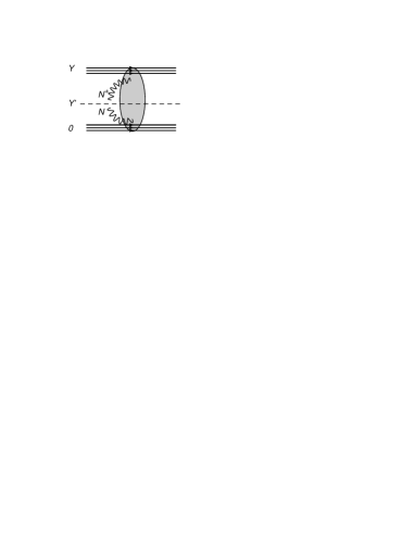
Figure 12: The graphical representation of the equation used for calculating the scattering amplitude using the $t$-channel unitarity.

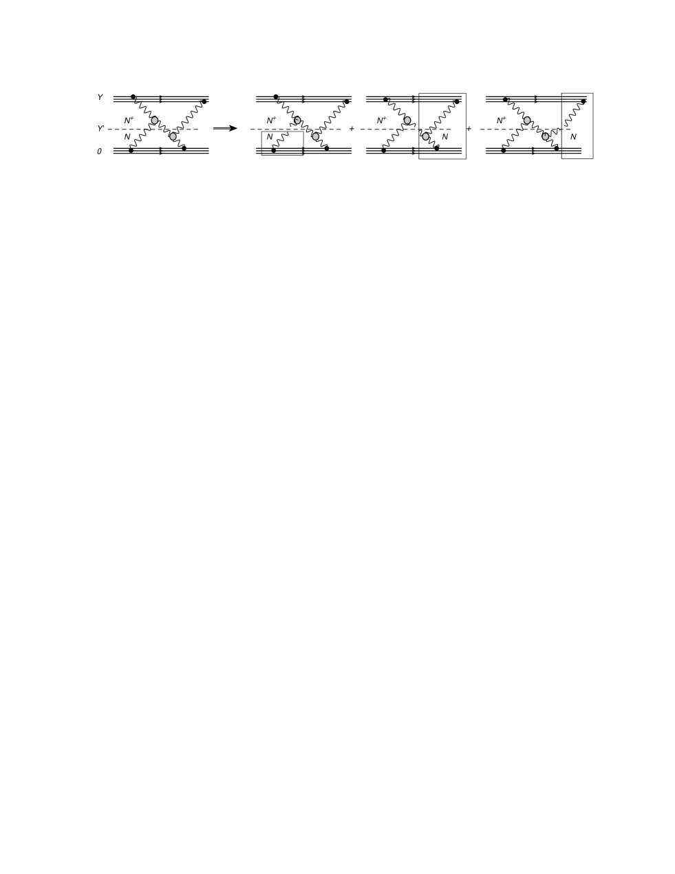
Figure 13: The example of the diagram which is described in terms of Eq. (4.120).

In Eq. (4) and Eq. (4.118) we use the same notation convention that was used in Eq. (3.103) and Eq. (3.104). The obvious way to calculate $\Omega$ (see Eq. (2.23)) is to find $N\left(z^{+}=z,Y^{\prime}=Y\right)$, since

$$\Omega/2\,\,=\,\ \int d^{2}x_{12}\,\tau_{pr}\,N\left(z^{+}=z,Y^{\prime}=Y\right)$$ (4.119)

However, in order to use Eq. (4.119) one needs to know the value of $N$ near to the saturation scale, whereas our approach has been developed inside of the two regions of saturation scales. We use the method related to $t$-channel unitarity (see Fig. 12) which was suggested and adjusted to high density QCD in Refs.[26, 34]. In this approach

$$\Delta\Omega\left(\zeta\right)/2\,\,=\,\ \int dz\,\Delta\,N\left(Y^{\prime},z\right)\,\Delta N\left(Y-Y^{\prime},z\right)\,$$ (4.120)

It should be stressed that the “net diagrams” of Fig. 1 possess the following remarkable property, that by cutting one BFKL Pomeron line we do not change the integration over the kinematic variables that describe other Pomerons. Therefore, these Pomerons are included in the description given by equation Eq. (4) and Eq. (4.118) for $N$ and $N^{+}$. In Fig. 13 we give an example of the diagram which is described in terms of Eq. (4.120). This figure illustrates the fact that the topology of the net diagrams (see Fig. 1) is very essential to the derivation of Eq. (4.120). The Pomeron loops cannot be taken into account using Eq. (4.120). The net diagrams have another remarkable feature, namely that all paths in the diagram that start from one nucleus, also finish at the other nucleus. In other words, there are no loops in the diagram. Each path can be cut at some value of rapidity, and contributes to Eq. (4.120). Keeping only the factor in the exponent we obtain that

$$\Delta\Omega\left(\zeta\right)/2\,\, = \,\ \int d\bar{z}\exp\Big{(}-{\cal Z}-{\cal Z}^{+}\Big{)}\,\$$

$$= \int d\bar{z}\exp\Big{(}-\,\sqrt{\frac{\bar{\alpha}_{S}^{2}\ln\left((Y-Y^{\prime})/\sqrt{\frac{1}{2}\zeta-\bar{z}}\right)}{\frac{1}{2}\zeta-\bar{z}}\,\left(Y-Y^{\prime}\right)^{2}}\,-\,\sqrt{\frac{\bar{\alpha}_{S}^{2}\ln\left(Y^{\prime}/\sqrt{\bar{z}}\right)}{\bar{z}}\,\left(Y^{\prime}\right)^{2}}\;\;\;\Big{)}$$

where $\bar{z}\,=\,z^{+}-\frac{1}{2}\lambda_{s}\,Y^{\prime}$. Integrating over $\bar{z}$ using the steepest decent method we obtain that the saddle point in the $\bar{z}$-integration is $\bar{z}_{SP}=\zeta/4$, which leads to

$$\Delta\Omega\left(\zeta\right)/2\,\,\,=\,\,\,\tilde{H}\,\exp\Big{\{}\,-\,\sqrt{\bar{\alpha}_{S}^{2}\ln\left(\frac{Y/2}{\sqrt{\zeta/4}}\right)}\frac{Y}{\sqrt{\zeta/4}}\;\Big{\}}$$ (4.122)

It is interesting to note that the dependence on $Y^{\prime}$ disappears, and the approach to the unitarity bound is much milder than in the case of the solution to the BK equation. Indeed, in the saturation region with two saturation scales $\Delta\Omega\,\propto\,\exp\Big{(}-\,Const\,\sqrt{Y}\Big{)}$ while for the BK equation $\Delta\Omega\,\propto\,\exp\Big{(}-\,Const\,Y^{2}\Big{)}$. The function $\tilde{H}$ absorbs all the pre-exponential factors that depend on $Y$ and impact parameters. The nucleus-nucleus scattering amplitude can be written using Eq. (2.23) - Eq. (2.25) in the form

$$\mbox{Im}A\left(Y;B\right)\,\,=\,\,1-\exp\Big{(}-\,\,\int d^{2}b\,d^{2}b^{\prime}\left(\tilde{S}_{A_{1}}\left(b\right)\,\tilde{S}_{A_{2}}\left(\vec{B}-\vec{b}\right)\,-\,\Delta\Omega\right)\Big{)}$$ (4.123)

where $b$ is the impact parameter of the nucleon inside of one nucleus and $B$ is the distance between the centers of two nucleons. $b^{\prime}$ in Eq. (4.123) is the impact parameter of the dipole inside of the nucleon. As we have discussed above, in our approach we integrated over this impact parameter. The typical value of $b^{\prime}$ is our new dimensional parameter, that determines the range of energy which we can reach within this approach. Generally speaking the average $b^{\prime}$ increases with energy, but we assume that $<b^{\prime}>\,\,\ll\,\,R_{A}$. This inequality determines the range of energies where we can trust our approach. The energy dependence of $<b>$ cannot be found in our approach, since in the framework of perturbative QCD, $<b>\propto s^{\Delta}$. However we know (see the Froissart theorem in ref. [35]) that $<b^{\prime}>$ can increase only logarithmically, but the parameters of such an increase will depend crucially on the non-perturbative parameter: the mass of the lightest hadron. The best estimate is to insert into Eq. (4.123) the experimental value of the inelastic cross section for the proton-proton interaction. In doing so we obtain

$$\mbox{Im}A\left(Y;B\right)\,\,=\,\,1-\exp\Big{(}\,-\,\sigma_{in}\left(pp\right)\,\int d^{2}b\tilde{S}_{A_{1}}\left(b\right)\,\tilde{S}_{A_{2}}\left(\vec{B}-\vec{b}\right)\Big{)}$$ (4.124)

It should be stressed that Eq. (4.124) flows naturally from our approach, whereas however it is certainly incorrect in the usual Glauber-Gribov [36] approximation (see Refs.[37]). However, we would like to stress that the form factors $\tilde{S}_{A_{i}}$ are different from the usual nucleus form factor $S_{A}\left(b\right)$. Indeed, $S_{A}\left(b\right)$ gives the number of nucleons that have impact parameter $b$ and it is equal to

$$S_{A}\left(b\right)\,=\,\int^{\infty}_{-\infty}dz\,\rho_{A}\left(z,b\right)$$ (4.125)

where $\rho$ is the density of nucleons in the nucleus. $\tilde{S}_{A}\left(b\right)$ is equal to

$$\tilde{S}_{A}\left(b\right)\,=\,\int^{R_{N}}_{-R_{N}}dz\,\rho_{A}\left(z,b\right)$$ (4.126)

and it characterizes the situation when all nucleons with the impact parameter $b$ interact as one.

5 Conclusions

In this paper we consider nucleus-nucleus scattering at high energies in the framework of the BFKL Pomeron Calculus, given by Eq. (2.14), which follows from the direct sum over Feynman diagrams. It turns out that for the dilute-dense system scattering, this approach gives the same results as other approaches, such as the dipole approach and the JIMWLK equation. Therefore, it seems reasonable to discuss nucleus scattering using the BFKL Pomeron Calculus, since other approaches have failed to successfully derive the set of equations for the dense-dense scattering amplitude. However, we would like to mention that in spite of the fact that we believe that the BFKL Pomeron Calculus describes the high energy interaction in QCD, we cannot exclude the opposite. In particular, it is possible that the four- Pomeron interaction could contribute at high energies. The most important result of this paper is the statement that at high energies, the equations in the BFKL Pomeron Calculus do not contradict either the $s$-channel unitarity, or the property of crossing symmetry. The main properties of our solution for the nucleus-nucleus scattering amplitude, can be summarized as follows.

1. The contribution of short distances to the opacity $\Omega$, dies at high energies.

2. The opacity tends to unity at high energies.

3. The main contribution that survives, originates from soft (long distance) processes for large values of the impact parameter.

The corrections to the opacity $\Omega=1-\Delta N$ that stem from short distances, have been discussed in this paper and it was shown that they behave differently from the corrections to the Balitsky-Kovchegov equation. Indeed, it turns out that $\Delta N\,\propto\,\exp\left(-Const\sqrt{Y}\right)$ while for the BK equation, $\Delta N\,\propto\,\exp\left(-ConstY^{2}\right)$.

The most salient result of this paper is the formula of Eq. (4.124) that describes nucleus-nucleus collisions. This formula is instructive, especially since in the usual Glauber-Gribov approach, there is no reason to expect that this formula works [37].

All of these above mentioned results are based on the BFKL Pomeron Calculus . It should be stressed that this Calculus and the action of Eq. (2.14) has been proven only at $N_{c}\,\gg\,1$. However, we should emphasize that the equivalence of this approach with other approaches (see refs. [10, 13] for example) that originate from the JIMWLK equation [7], have not been proven. It should be stressed that the two strategies reflect two different fundamental features of QCD, namely that the BFKL Pomeron Calculus satisfies, by construction, the $t$-channel unitarity whereas JIMWLK-based approaches are precise from the point of view of $s$-channel unitarity. In general Eq. (2.3) and Eq. (2.3) give the equations for the dense-dense system of scattering, in the mean field approximation which replaces the BK equation, while the solution that was found in this paper has the same legacy as the solution to the BK equation deeply in the saturation region, given in Ref. [31].

However, the mean field approximation cannot be trusted at extremely high energies. Strictly speaking starting from $Y=Y_{m}$ where $\alpha_{S}^{2}\exp\Big{(}\omega(0)Y_{m}\Big{)}=1$, both solutions are not valid and we need to take into account all kind of enhanced diagrams (see Fig. 7-b for example). However, to calculate such diagrams we need to find the Green function of the Pomeron in the mean field approximation. Since at $Y=Y_{m}$ these solutions give the amplitude which is close to the unitarity boundary , the Green function can be small show that such a scenario looks very plausible. Therefore, the problem of taking into account of Pomeron loops could be not important for the understanding of the phenomena of saturation.

References

- [1] L. V. Gribov, E. M. Levin and M. G. Ryskin, Phys. Rep. 100 (1983) 1.
- [2] A. H. Mueller and J. Qiu, Nucl. Phys. B268 (1986) 427.
-
[3]
L. McLerran and R. Venugopalan,
Phys. Rev. D49 (1994) 2233, 3352; D50 (1994) 2225;
D53 (1996) 458;
D59 (1999) 09400. - [4] A. H. Mueller, Nucl. Phys. B 415, 373 (1994); Nucl. Phys. B 437 (1995) 107 [arXiv:hep-ph/9408245].
- [5] I. Balitsky, [arXiv:hep-ph/9509348]; Phys. Rev. D60, 014020 (1999) [arXiv:hep-ph/9812311]
- [6] Y. V. Kovchegov, Phys. Rev. D60, 034008 (1999), [arXiv:hep-ph/9901281].
- [7] J. Jalilian-Marian, A. Kovner, A. Leonidov and H. Weigert, Phys. Rev. D59, 014014 (1999), [arXiv:hep-ph/9706377]; Nucl. Phys. B504, 415 (1997), [arXiv:hep-ph/9701284]; J. Jalilian-Marian, A. Kovner and H. Weigert, Phys. Rev. D59, 014015 (1999), [arXiv:hep-ph/9709432]; A. Kovner, J. G. Milhano and H. Weigert, Phys. Rev. D62, 114005 (2000), [arXiv:hep-ph/0004014] ; E. Iancu, A. Leonidov and L. D. McLerran, Phys. Lett. B510, 133 (2001); [arXiv:hep-ph/0102009]; Nucl. Phys. A692, 583 (2001), [arXiv:hep-ph/0011241]; E. Ferreiro, E. Iancu, A. Leonidov and L. McLerran, Nucl. Phys. A703, 489 (2002), [arXiv:hep-ph/0109115]; H. Weigert, Nucl. Phys. A703, 823 (2002), [arXiv:hep-ph/0004044].
- [8] E. Gotsman, E. Levin, U. Maor and E. Naftali, Nucl. Phys. A 750 (2005) 391 [arXiv:hep-ph/0411242].
- [9] M. A. Braun, Phys.Lett. B 483 (2000) 115, [arXiv:hep-ph/0003004]; Eur.Phys.J C 33 (2004) 113 [arXiv:hep-ph/0309293] ; Phys. Lett. B 632 (2006) 297, [Eur. Phys. J. C 48 (2006) 511], [arXiv:hep-ph/0512057].
- [10] T. Altinoluk, A. Kovner, M. Lublinsky and J. Peressutti, JHEP 0903 (2009) 109 [arXiv:0901.2559 [hep-ph]]; A. Kovner and M. Lublinsky, Phys. Rev. Lett. 94 (2005) 181603 [arXiv:hep-ph/0502119]; Phys. Rev. D 71 (2005) 085004 [arXiv:hep-ph/0501198].
- [11] E. Levin and M. Lublinsky, Nucl. Phys. A 763 (2005) 172 [arXiv:hep-ph/0501173].
- [12] J. P. Blaizot, E. Iancu, K. Itakura and D. N. Triantafyllopoulos, Phys. Lett. B 615 (2005) 221 [arXiv:hep-ph/0502221].
- [13] Y. Hatta, E. Iancu, L. McLerran, A. Stasto and D. N. Triantafyllopoulos, Nucl. Phys. A 764 (2006) 423 [arXiv:hep-ph/0504182].
- [14] C. Marquet, A. H. Mueller, A. I. Shoshi and S. M. H. Wong, Nucl. Phys. A 762 (2005) 252 [arXiv:hep-ph/0505229].
- [15] E. Levin, J. Miller and A. Prygarin, Nucl. Phys. A 806 (2008) 245 [arXiv:0706.2944 [hep-ph]].
- [16] E. Levin, Nucl. Phys. B 453 (1995) 303 [arXiv:hep-ph/9412345].
- [17] E. A. Kuraev, L. N. Lipatov, and F. S. Fadin, Sov. Phys. JETP 45, 199 (1977); Ya. Ya. Balitsky and L. N. Lipatov, Sov. J. Nucl. Phys. 28, 22 (1978).
- [18] L. N. Lipatov, Phys. Rep. 286 (1997) 131; Sov. Phys. JETP 63 (1986) 904 and references therein.
- [19] M. Kozlov, E. Levin and A. Prygarin, Nucl. Phys. A 792, 122 (2007) [arXiv:0704.2124 [hep-ph]]; “The BFKL pomeron calculus: Probabilistic interpretation and high energy amplitude,” arXiv:hep-ph/0606260.
- [20] S. Bondarenko and L. Motyka, Phys. Rev. D 75 (2007) 114015 [arXiv:hep-ph/0605185].
- [21] S. Bondarenko and M. A. Braun, Nucl. Phys. A 799 (2008) 151 [arXiv:0708.3629 [hep-ph]].
- [22] E. Gotsman, A. Kormilitzin, E. Levin and U. Maor, Nucl. Phys. A 842 (2010) 82 [arXiv:0912.4689 [hep-ph]].
- [23] A. Schwimmer, Nucl. Phys. B 94 (1975) 445.
- [24] R.J.Glauber, in “Lectures in Theoretical Physics”, edited by by W. E. Britten et al. (Interscience, New York) 1, (1959) 315.
- [25] A. Kovner and U. A. Wiedemann, Phys. Lett. B 551 (2003) 311 [arXiv:hep-ph/0207335]; Phys. Rev. D 66 (2002) 034031 [arXiv:hep-ph/0204277]; Phys. Rev. D 66 (2002) 051502 [arXiv:hep-ph/0112140].
- [26] A. H. Mueller and A. I. Shoshi, Nucl. Phys. B 692 (2004) 175 [arXiv:hep-ph/0402193].
- [27] A. H. Mueller, Nucl. Phys. A 724 (2003) 223 [arXiv:hep-ph/0301109];Nucl. Phys. B 558 (1999) 285 [arXiv:hep-ph/9904404]; D. Kharzeev, E. Levin and L. McLerran, Phys. Lett. B 561 (2003) 93 [arXiv:hep-ph/0210332]; E. M. Levin and M. G. Ryskin, Nucl. Phys. B 304 (1988) 805; Sov. J. Nucl. Phys. 41 (1985) 472.
- [28] A. H. Mueller and D. N. Triantafyllopoulos, Nucl. Phys. B640 (2002) 331 [arXiv:hep-ph/0205167]; D. N. Triantafyllopoulos, Nucl. Phys. B648 (2003) 293 [arXiv:hep-ph/0209121].
- [29] S. Munier and R. Peschanski, Phys. Rev. D70 (2004) 077503; D69 (2004) 034008 [arXiv:hep-ph/0310357]; Phys. Rev. Lett. 91 (2003) 232001 [arXiv:hep-ph/0309177].
- [30] V. A. Khoze, A. D. Martin, M. G. Ryskin and W. J. Stirling, Phys. Rev. D 70 (2004) 074013 [arXiv:hep-ph/0406135].
- [31] E. Levin and K. Tuchin, Nucl. Phys. B 573 (2000) 833 [arXiv:hep-ph/9908317].
- [32] I. Gradstein and I. Ryzhik, ”Tables of Series, Products, and Integrals”, Verlag MIR, Moskau,1981.
- [33] E. Levin and K. Tuchin, Nucl. Phys. A 693 (2001) 787 [arXiv:hep-ph/0101275].
- [34] E. Iancu and A. H. Mueller, Nucl. Phys. A730 (2004) 460 [arXiv:hep-ph/0308315]; 494 [arXiv:hep-ph/0309276].
-
[35]
M. Froissart,
Phys. Rev. 123 (1961) 1053;
A. Martin, “Scattering Theory: Unitarity, Analitysity and Crossing.” Lecture Notes in Physics, Springer-Verlag, Berlin-Heidelberg-New-York, 1969. - [36] R.J. Glauber, In: Lectures in Theor. Phys., v. 1, ed. W.E. Brittin and L.G. Duham. NY: Intersciences, 1959; Gribov, V. N., Sov. Phys. JETP 29 483, [Zh. Eksp. Teor. Fiz. 56 892 (1969)]; Sov. Phys. JETP 30 709 [Zh. Eksp. Teor. Fiz. 57 (1969) 1306].
- [37] A. Kaidalov, Nucl. Phys. A 525 (1991) 39; K. G. Boreskov and A. B. Kaidalov, Sov. J. Nucl. Phys. 48 (1988) 367 [Yad. Fiz. 48 (1988) 575]; Acta Phys. Polon. B 20 (1989) 397 and references therein.
- [38] M. A. Braun, A. Tarasov, [arXiv:1010.2586 [hep-ph]].