Optimizing an Organized Modularity Measure for Topographic Graph Clustering: a Deterministic Annealing Approach

Abstract

This paper proposes an organized generalization of Newman and Girvan’s modularity measure for graph clustering. Optimized via a deterministic annealing scheme, this measure produces topologically ordered graph clusterings that lead to faithful and readable graph representations based on clustering induced graphs. Topographic graph clustering provides an alternative to more classical solutions in which a standard graph clustering method is applied to build a simpler graph that is then represented with a graph layout algorithm. A comparative study on four real world graphs ranging from 34 to 1 133 vertices shows the interest of the proposed approach with respect to classical solutions and to self-organizing maps for graphs.

1 Introduction

Large and complex graphs are natural ways of describing real world systems that involve interactions between objects: persons and/or organizations in social networks, articles in citation networks, web sites on the world wide web, proteins in regulatory networks, etc. [30]. However, the complexity of real world graphs limits the possibilities of exploratory analysis: while many graph drawing and graph visualization methods have been proposed [9, 21], displaying a graph with a few hundred vertices in a meaningful way remains difficult.

A way to tackle this scalability issue is to simplify a graph prior its drawing. This can be done by finding clusters of vertices via a graph clustering method [42]: rather than representing the original graph, the visualization is restricted to the clusters themselves. More precisely, the graph induced by the clustering is used: each cluster forms a vertex, while edges between clusters are induced by edges between the vertices they contain. As illustrated in the survey paper [21], numerous implementations of this simple idea can be done, namely all the pairwise combinations between graph clustering methods and graph visualization methods (see also, e.g., [11] for recent work on planar clustered graphs and [5] for weighted graphs).

Rather than relying on a generic graph clustering algorithm, we propose in this paper to build a clustering of a graph that is adapted to a visualization of the graph induced by the clustering. We follow the general principal of topographic mapping initiated by Prof. Kohonen with the Self Organizing Map (SOM, [26]): a SOM builds a clustering of a dataset in homogeneous and separated clusters that are in addition arranged on a geometrical structure chosen a priori; points assigned to close clusters in the prior structure are close in the original space.

Our method is built on an organized generalization of the popular modularity measure [34] for graph clustering. Following the SOM rationale, the organized modularity uses a prior structure to build topologically aware clusters: nodes assigned to close clusters in the prior structure are more likely to be connected in the original graph than nodes assigned to distant clusters. As for the SOM [45, 46], using a two dimensional regular grid as a prior structure enables straightforward visualization of the graph induced by the clustering.

While the modularity has interesting properties over other graph cut measures [31, 32, 33, 29], especially in the visualization context [36], it has two drawbacks shared with its organized generalization. Firstly, maximizing the (organized) modularity is a combinatorial problem and there is no simple prototype based alternating optimization scheme as available for the SOM and its non Euclidean variants [20, 4, 47, 48]. Following [29] for the modularity, we rely on a deterministic annealing approach [41] to solve this problem. Secondly, maximizing the (organized) modularity measure tends to miss small clusters, i.e., to aggregate them in large clusters [13]. To limit this effect, we also propose to use the intermediate states of the deterministic annealing algorithm to build finer clusterings than the one with maximal organized modularity. Combined with the prior structure, those clusterings give refined views of the graph induced by the clustering. In summary our contribution is twofold: we introduce an organized modularity measure and we use deterministic annealing to build fair and simplified visualizations of a graph, that are based on a clustering of the vertices.

The rest of this paper is organized as follows: Section 2 details the clustering approach to graph visualization, recalls the modularity definition and introduces its topographic generalization (the organized modularity). Section 3 presents the deterministic annealing scheme used to optimize the organized modularity. Section 4 describes the proposed graph visualization methodology and shows in particular how to leverage the intermediate results of the optimization algorithm to produce fuzzy layouts that limit the resolution effect induced by modularity maximization. Section 5 analyses in detail the behavior of the proposed method on a simple graph, Zachary’s Karate club social network [54]. Finally, Section 6 demonstrates the practical interests of the method on three larger real world graphs. Technical derivations are gathered in an appendix.

2 Topographic graph clustering

2.1 Graph clustering for visualization

Cognitive scalability can be brought to graph visualization methods [21] via graph clustering [42]: the rationale is to draw the smaller and hopefully simpler graph induced by the clustering instead of the original graph. Let us define more precisely this idea.

We consider given a non oriented graph $G$ with $N$ vertices (or nodes), $V(G)=\{1,\ldots,N\}$ and $A$ weighted edges ($A(G)$ is the set of edges). The (symmetric) weight matrix is denoted by $W$, and $W_{ij}$ is the non negative weight between vertex $i$ and vertex $j$ ($W_{ij}=0$ when $(i,j)\not\in A(G)$). A clustering of $V(G)$ into $C$ clusters $(C_{k})_{1\leq k\leq C}$ induces a new non oriented graph $G_{C}$ defined as follows: each cluster is associated to a vertex in $G_{C}$, i.e., $V(G_{C})=\{1,\ldots,C\}$ and a pair $(i,j)$ belongs to the edge set $A(G_{C})$ if and only if there is $(k,l)\in A(G)$ such that $k\in C_{i}$ and $l\in C_{j}$. $G_{C}$ is weighted and the corresponding weight matrix is denoted $W^{C}$. The weights are defined by $W^{C}_{ij}=\sum_{k\in C_{i},l\in C_{j}}W_{kl}$ (for $i\neq j$).

The present paper focuses on the following graph visualization strategy: a clustering $C$ of the original graph $G$ is constructed and a graph visualization method is applied to $G_{C}$. In general, the visual representation is completely unaware of the way $G_{C}$ has been produced: this is a simpler setting than the one of e.g. [11, 5] in which the proposed algorithms aim at representing a so-called clustered graph. In this latter context, the ultimate goal is to visualize the complete original graph in a way that respects the (hierarchical) clustering structure. The clustering is used in this case both as a way to circumvent algorithmic difficulties (e.g., the cost of some force directed methods) and as a structural organization principle. In the present paper, the clustering method makes “a meaningful coarse graining of the graph” (to quote [34]) and produces a new graph which will be the main target of the visualization method.

The solution chosen in this paper is also related to but quite different from the clustered layout strategy [21]. In this framework, one aims at producing a visualization of a graph in which vertices that belong to a given cluster are close, while distinct clusters remain separated. Clusters are generally a by product of those algorithms rather than given beforehand (see, e.g., [35] for a recent example of such a method).

In practice, we target visualization methods in which each vertex of the new graph $G_{C}$ is represented by a glyph (e.g., a disk) while each edge is drawn as a straight segment between the corresponding vertices’ glyphs (we do not consider more sophisticated drawing, for instance with bends). Rendering hints can be used to convey information about the original graph to the user: the surface occupied by a glyph can be proportional to the size of the corresponding cluster, while the thickness of a segment can encode the weight associated to the corresponding edge.

2.2 Quality measures

In order to be useful, a graph visualization produced via the chosen clustering framework must be both readable and faithful. The readability issue is common to all graph visualization algorithms and has been a matter of research and debate in the graph visualization community with a particular focus on aesthetic criteria, such as bend minimization, symmetry, etc. [9, 21, 38]. Experimental studies show that a minimal number of edge crossings is one of the most important quality criteria for readability (see e.g. [50]). Please note however that there is no consensus on what other readability criteria should be used to evaluate the quality of a graph representation beyond direct task based user studies. In particular, neighborhood rank preservation measures used to assess the quality of nonlinear projection methods [28] are likely to be irrelevant in the graph context: as showed in [12], displaying the edges of a graph has a major influence on the way proximities between nodes are inferred by users from the visualization.

The faithfulness issue is more specific to the cluster based visualization: as the final representation of the graph hides most of its structure, inference on the drawing can be misleading. More precisely, there are two potential problems induced respectively by the vertices and the edges in the $G_{C}$ graph. The first difficulty is that the internal connectivity structure of clusters is hidden by the glyph based representation: while color and/or shape hints could be used to give an idea of the density of connections between the vertices that have been put in a given cluster, the actual connection pattern is lost. A similar problem happens for connection patterns between vertices of distinct clusters: as the associated edges are summarized by a single edge between the induced vertices, there is no way to infer how individual vertices are connected in the original graph.

Therefore, building a faithful clustering of a graph amounts to balancing two criteria that are somewhat contradictory: on the one hand, the density of each cluster should be maximized, but on the other hand the connectivity pattern between two vertices of distinct clusters should be independent of the vertices. Intuitively, a dense cluster with a low outside connectivity is likely to have a rather complex outside connectivity pattern: if all vertices in a cluster were connected to e.g., a single outside vertex, then it might make sense to assign this vertex to the cluster. In addition, enforcing a simple between cluster connectivity has no reason to reduce edge crossing, while within cluster density maximization should on the contrary reduce the number of between cluster connection and therefore improve the readability of the graph.

It seems therefore natural to focus on within cluster density maximization as this solution should lead to a readable graph with a controlled impact on the faithfulness of the representation. Among the clustering quality criteria that favor within cluster density (see [42]), we focus on the modularity introduced by Newman and Girvan in [34]. Let us denote $k_{i}=\sum_{j}W_{ij}$ the degree of vertex $i$ and $m=\frac{1}{2}\sum_{i,j}W_{ij}$ the total weight of the graph. Then the modularity of the clustering $(C_{k})_{1\leq k\leq C}$ of $G$ is

$$Q\left((C_{k})_{1\leq k\leq C}\right)=\frac{1}{2m}\sum_{k=1}^{C}\sum_{i,j\in C_{k}}\left(W_{ij}-P_{ij}\right),$$ (1)

where $P$ is a $N\times N$ symmetric matrix given by $P_{ij}=\frac{k_{i}k_{j}}{2m}$.

The rationale of the measure is to compare the weight of a link between two vertices in a cluster, $W_{ij}$, to a simple random model, $P_{ij}$, in which the weights are proportional to the degrees of the vertices and independent of the clusters. A good clustering tends to cluster vertices that are more connected that one expects based solely on the degrees of the vertices: this corresponds to $W_{ij}>P_{ij}$ and to higher values of $Q(M)$. Maximizing the modularity tends therefore to produce dense clusters, but only when they are meaningful as measured by a deviation from the simple random model.

The modularity is a rather successful quality measure for graph clustering, especially compared to other graph cut like measures [31, 32, 33, 29]. In addition, [36] has recently shown that there is a strong link between clusterings induced by modularity maximization and those obtained with some versions of the clustered layout strategy described previously. The modularity seems therefore to be a good candidate for the topographic extension studied in this paper. However, this measure suffers from a resolution problem [13]: maximizing the modularity may fail to identify small but meaningful clusters of nodes. We will tackle this problem by leveraging both the chosen optimization algorithm and the prior structure introduced below (see Section 4.2 for details). It should be noted in addition that the main concepts and techniques used in this paper are quite independent from the actual quality measure. In particular most graph cut based measures [42] could be handled in a similar way as we proceed with modularity.

2.3 Organized modularity

The main limitation of graph clustering for visualization is that the two phases of the methodology are generally completely independent: the clustering method is not explicitly designed to help the subsequent visualization method. We propose in this paper to address this limitation via a specific quality measure for the clustering phase.

Following the SOM rationale, we derive an organized version of the modularity. We assume given a prior structure (in $\mathbb{R}^{2}$) which is represented by a symmetric $C$ by $C$ matrix $S$ of prior similarities between clusters such that $S_{kk}=1$ for all $k=1,\ldots,C$. For instance $S_{kl}=\exp(-\sigma\|\mathbf{x}_{k}-\mathbf{x}_{l}\|^{2})$ where $\mathbf{x}_{k}$ is the prior position of cluster $C_{k}$ in $\mathbb{R}^{2}$. Then the organized modularity of the clustering $(C_{k})_{1\leq k\leq C}$ of $G$ is

$$O\left((C_{k})_{1\leq k\leq C}\right)=\frac{1}{2m}\sum_{i,j}S_{c(i)c(j)}\left(W_{ij}-P_{ij}\right),$$ (2)

where $c(i)$ is the index of the cluster to which the vertex $i$ is assigned.

In the standard modularity, the term $W_{ij}-P_{ij}$ is taken into account only when $i$ and $j$ belong to the same cluster. In the organized version, this term is always taken in account, but with a weight $S_{c(i)c(j)}$ equal to the prior similarity between $C_{c(i)}$ and $C_{c(j)}$. This favors proximity in the prior structure for connected clusters. If there are indeed significant connections between vertices in two clusters $C_{k}$ and $C_{l}$ (i.e., $W_{ij}-P_{ij}>0$), then the value of $O$ will be higher if $S_{kl}$ is high than if it is low. This is similar to the SOM principle in which a prototype has to be close to observations assigned to its unit but also, to a lesser extent, to observations assigned to neighboring units in the prior structure.

Maximizing $O\left((C_{k})_{1\leq k\leq C}\right)$ gives a graph clustering that can be used to coarsen the original graph prior a standard visualization algorithm, as explained in Section 2.1. In addition, the prior structure gives a natural layout for the clustered graph: nodes of this new graph can be drawn at their corresponding positions on the grid.

3 Organized modularity maximization

3.1 Modularity maximization

The main difficulty with (organized) modularity maximization is that it is a discrete optimization problem for which there is no simple alternate minimization scheme (contrarily to the SOM or the $k$-means, for instance). Deriving fast modularity maximization algorithms that produce acceptable solutions has been an important research topic since the introduction of this quality measure (this is generally the case for all graph clusteringing measures). The best compromise between computational load and quality seems to be currently achieved by some type of heuristic algorithms that coarsen the graph in an iterative and multi-level way [3, 37].

In the present paper, we use a quite different approach which is more adapted to the organized modularity defined in the previous Section. Following [29], we propose to maximize the (organized) modularity via a deterministic annealing (DA) approach [41]. As pointed out in [29], the main advantage of DA over simulated annealing (as used by, e.g., [40] in the graph clustering context) is the speed of the former: deterministic annealing can use aggressive annealing schedules with a relatively small number of iterations compared to simulated annealing. In addition, intermediate results of DA can be used to limit the resolution effect induced by modularity maximization, as will be shown in Section 4.2.

To ease the derivation of the DA algorithm for modularity maximization, we use an assignment matrix notation for clusterings. An assignment matrix $M$ for a clustering of $\{1,\ldots,N\}$ in $C$ clusters is a $N\times C$ matrix with entries in $\{0,1\}$ such that $\sum_{k=1}^{C}M_{ik}=1$ for all $i$. In other words, $M_{ik}$ is equal to 1 if and only if $i$ is assigned to cluster $C_{k}$. We denote $\mathcal{M}$ the set of all valid assignment matrices for a clustering of $\{1,\ldots,N\}$ in $C$ clusters ($N$ and $C$ will be given by the context). Please note that we do not constrain an assignment matrix to have non empty clusters.

The modularity and the organized modularity of an assignment matrix $M$ are given respectively by:

$$Q(M) = \frac{1}{2m}\sum_{i,j}\sum_{k}M_{ik}M_{jk}\left(W_{ij}-P_{ij}\right)$$ (3)

$$O(M) = \frac{1}{2m}\sum_{i,j}\sum_{k,l}M_{ik}S_{kl}M_{jl}\left(W_{ij}-P_{ij}\right)$$ (4)

If $B$ is the $N\times N$ symmetric matrix defined by

$$B_{ij}=\begin{cases}0&\text{if }i=j\\ \frac{1}{2m}\left(W_{ij}-P_{ij}\right)&\text{if }i\neq j.\end{cases}$$ (5)

then, maximizing $O(M)$ is equivalent to maximizing

$$F(M)=\sum_{i,j}\sum_{k,l}M_{ik}S_{kl}M_{jl}B_{ij}$$ (6)

as shown in Section A.1. Finally, it should be noted that by using the identity matrix for $S$, one recovers the modularity: the algorithm derived for the maximization of $F(M)$ will therefore apply to both the standard modularity and the organized version.

3.2 Deterministic annealing and mean field approximation

Deterministic annealing tries to solve the complex combinatorial problem of maximizing a function $F$ defined on a finite (but large) space $\mathcal{M}$ via an analysis of the Gibbs distribution obtained as the asymptotic regime of a classical simulated annealing [24, 7] or via the principal of maximum entropy [41]. In our case, the Gibbs distribution for temperature $\frac{1}{\beta}$ is

$$P(M)=\frac{1}{Z_{P}}\exp(\beta F(M)),$$ (7)

where the normalization constant $Z_{P}$ is given by $Z_{P}=\sum_{M\in\mathcal{M}}\exp(\beta F(M))$ (the sum ranges over the full space $\mathcal{M}$).

The main idea of DA is to compute the expectations of the assignment matrix at a fixed temperature with respect to the Gibbs distribution, i.e., the $\mathbb{E}\left(M_{ik}\right)$, and then to decrease the temperature while tracking the evolution of the expectations (in simulated annealing, the Gibbs distribution is sampled rather than studied via expectation).

Unfortunately, $F$ is not linear with respect to $M$ and computing $Z_{P}$ and $P$ is therefore difficult: one should resort on an exhaustive exploration of $\mathcal{M}$ which is computationally infeasible. Following previous work on similar topics, we approximate $P$ by a distribution that factorizes (see e.g., [22, 18]). This corresponds to approximating the interaction between say $M_{ik}$ and all the other variables via a mean field $E_{ik}$. Then we compute the expectation of the assignment matrix with respect to the approximating distribution.

More precisely, we consider the bi-linear cost function $U(M,E)=\sum_{i}\sum_{k}M_{ik}E_{ik}$ where $E$ is the mean field, a $N$ by $C$ matrix of partial assignment costs. For a fixed temperature $\frac{1}{\beta}$, we look for a mean field $E$ that gives a distribution $R(M,E)=\frac{1}{Z_{R}(E)}\exp(\beta U(M,E))$ close to $P(M)$, in the sense that the Kullback-Leibler divergence $KL(R|P)$ between $R$ and $P$ is minimal, with $KL(R|P)=\sum_{M}R(M,E)\ln\frac{R(M,E)}{P(M)}$ (this corresponds to a variational approximation of $P$ [23]).

At a minimum, the gradient of $KL(R|P)$ with respect to $E$ is zero. This leads to the following classical mean field equations (see Appendix A.2 for details):

$$\frac{\partial\mathbb{E}_{R}\left(F(M)\right)}{\partial E_{jl}}=\sum_{k}\frac{\partial\mathbb{E}_{R}\left(M_{jk}\right)}{\partial E_{jl}}E_{jk},\ \forall j,l.$$ (8)

They are obtained using the main consequence of the mean field approximation, namely the independence between $M_{ik}$ and $M_{jl}$ for $i\neq j$ under the distribution $R$, i.e., the fact that $\mathbb{E}_{R}\left(M_{ik}M_{jl}\right)=\mathbb{E}_{R}\left(M_{ik}\right)\mathbb{E}_{R}\left(M_{jl}\right)$ for $i\neq j$.

To solve the mean field equations, we use a EM-like approach. We consider the $\mathbb{E}_{R}\left(M_{ik}\right)$ fixed and solve the equations for $E_{jl}$ (maximization phase). Then we compute the new values of the $\mathbb{E}_{R}\left(M_{ik}\right)$ (expectation phase). This latter phase leads to the very simple standard deterministic annealing update rule:

$$\mathbb{E}_{R}\left(M_{ik}\right)=\frac{\exp(\beta E_{ik})}{\sum_{l}\exp(\beta E_{il})}.$$ (9)

Moreover, the independence property recalled above gives

$$\mathbb{E}_{R}\left(F(M)\right)=\sum_{i\neq j}\sum_{k,l}\mathbb{E}_{R}\left(M_{ik}\right)S_{kl}\mathbb{E}_{R}\left(M_{jl}\right)B_{ij}.$$

Then, some straightforward calculations (see Appendix A.3 for details) show that equation (8) is fulfilled if the mean field is given by

$$E_{jk}=2\sum_{i\neq j}\sum_{l}\mathbb{E}_{R}\left(M_{il}\right)S_{kl}B_{ij},$$ (10)

or, in matrix notations, $E=B\mathbb{E}_{R}\left(M\right)S$, using the symmetry of $B$ and $S$.

3.3 Phase transition and final algorithm

It is well known that deterministic annealing goes through several phase transitions when the temperature is decreased [41, 17, 22]. In order to choose an adapted annealing schedule, i.e., an increasing series of $(\beta_{l})_{1\leq l\leq L}$ that is used to track the evolution of $\mathbb{E}_{R}\left(M\right)$, it is important to find at least the first phase transition.

At the limit of infinite temperature ($\beta=0$), it can be shown (see Appendix A.4) that the following mean field

$$E^{0}_{jk}=\frac{2}{C}\sum_{i\neq j}B_{ij}\sum_{l}S_{kl},$$ (11)

is a fixed point of the $EM$ like scheme (i.e., of equations (9) and (10)). The corresponding assignment expectations are uniform, i.e.

$$\mathbb{E}_{R}\left(M_{ik}^{0}\right)=\frac{1}{C}.$$ (12)

An analysis of the stability of the EM-like scheme (conducted in Appendix A.4) shows that the fixed point $E^{0}$ is stable when the temperature $\frac{1}{\beta}$ is higher than the critical temperature $T_{0}=\frac{2\lambda_{B}\lambda_{S}}{C}$, where $\lambda_{B}$ and $\lambda_{S}$ are the spectral radii, i.e., the largest eigenvalues in absolute value, respectively of $B$ and $S$. The first phase transition will therefore happen when the temperature becomes lower than this limit. It should be noted that the critical temperature is a very conservative estimation of the temperature of the first phase transition, as it corresponds to a worst case analysis of the stability of the fixed point.

Algorithm 1 Deterministic annealing for organized modularity maximization

1:  initialize $E$ to $E^{0}$ from equation (11)

2:  $T_{0}\leftarrow\frac{2\lambda_{B}\lambda_{S}}{C}$ {critical temperature}

3:  $T\leftarrow\alpha T_{0}$

4:  for $l=1$ to $L$ do {annealing loop}

5:     $E\leftarrow E+\varepsilon$ {noise injection}

6:     repeat {EM-like phase}

7:        compute $\mathbb{E}_{R}\left(M_{ik}\right)$ using equation (9) with $\beta=\frac{1}{T}$

8:        compute $E$ using equation (10)

9:     until convergence of $E$

10:     $T\leftarrow\gamma T$

11:  end for

12:  threshold $\mathbb{E}_{R}\left(M\right)$ into an assignment matrix

To derive the final Algorithm 1, we follow [41] rather than [29]. We use in particular the perturbation idea of [41]: each time the temperature is lowered, some noise is injected in the mean field before running the EM-like scheme. This method favors phase transitions and symmetric breaks that are needed for a proper convergence.

Deterministic annealing is very robust and quite insensitive to the parameters that appear in Algorithm 1:

• $L$ is the number of outer iterations, i.e., the number of temperatures considered during the annealing process (a typical value is $N$, the size of the graph);

• $\alpha>1$ is the relative starting temperature above the critical temperature (typically $1.1$);

• $\gamma$ is the damping factor of the temperature (typically chosen such that the final temperature is $0.1T_{0}$);

• for the noise $\varepsilon$, we used a random multiplicative factor chosen uniformly in $[0.995,1.005]$ for each component of $E$;

• the EM-like phase is considered to be stable when the mean squared difference between the components of two values of $E$ is below the square root of the machine precision (or after 500 iterations).

Finally, the computation cost of the algorithm remains reasonable: the costly operation is the product $B\mathbb{E}_{R}\left(M\right)$. As explained in [31], one can leverage the structure of $B$ to obtain a fast matrix multiplication. Indeed $B$ is made from $W$ the weight matrix and $P$ the degree matrix. Computing $Wx$ costs $O(A)$ operations (where $A$ is the number of edges of the graph), while $Px$ can be computed in $O(N)$ operations ($N$ is the number of vertices) exploiting the definition of $P$. Therefore computing $B\mathbb{E}_{R}\left(M\right)$ costs $O(C(A+N))$. Then computing the product of $B\mathbb{E}_{R}\left(M\right)$ by $S$ is a $O(NC^{2})$ operation while applying equation (9) costs $O(NC)$. The total cost of one iteration of Algorithm 1 is therefore $O(CA+C^{2}N)$. Computing the critical temperature can be done quite efficiently via the Lanczos method [16] in $O(N(A+N))$ but in fact only a very rough estimate of the spectral radius is needed. Therefore, a few iterations of a power method should be enough to give a reasonable initial temperature. In practice, the computational cost of the method makes it suitable for graphs with a few thousands vertices as long as there are not too dense.

4 Graph visualization methodology

In principle, the proposed graph visualization methodology is rather straightforward and strongly related to e.g., exploratory data analysis with the SOM. We choose a regular grid as a prior structure and use Algorithm 1 to find an optimal clustering with respect to the organized modularity defined by equation (4). Then, as explained in Section 2.1, we display the clustering induced graph: we do not need a graph layout algorithm in this phase as each cluster has a dedicated position in the grid.

In practice, some parameters need to be carefully chosen to provide a meaningful visualization. In addition, (organized) modularity maximization faces a problem of limited resolution and leads sometimes to oversimplified clustering induced graph. We describe in this Section the proposed solutions to those issues.

4.1 Parameter tuning

The internal parameters of Algorithm 1 described in Section 1 do not request any particular tuning and the guidelines provided should in general give satisfactory results. On the contrary, the quality of the visual representation strongly depends on the prior structure, both in terms of the size of grid itself and in terms of the $S$ matrix. Those parameters should be optimize as automatically as possible. The general principle consists first in defining a finite set of acceptable prior structures and then in selecting the best one via some quality criterion.

Our practical goal is to end up with readable graphs: we consider therefore small prior structures, for instance square grids with an absolute maximum of 10 nodes per dimension (i.e., up to 100 clusters). The entries of the matrix $S$ are calculated via a SOM like equation

$$S_{ij}=H(\lambda\|x_{i}-x_{j}\|),$$ (13)

where $x_{i}$ is the position of cluster $i$ in the prior structure and $H$ is either $H(t)=\exp(-t^{2})$ (exponential decrease) or $H(t)=\max(0,1-t)$ (linear decrease). The scaling parameter $\lambda$ is used to tune the neighboring influence and can be chosen so as to include from zero neighbor to a complete influence of all clusters on each other.

Unfortunately, as recalled in Section 2.2, there is no universally accepted quality criterion for graph visualization. Moreover, the case of clustered visualization naturally corresponds to a trade-off between internal and external connectivity uniformity. To handle this trade-off we propose to rely on dual objectives optimization principles. More precisely, we use the standard modularity measure to assess clustering quality and the number of edge crossing to assess visual quality. Rather than combining the measures to select one value of the parameters of the prior structure, we consider Pareto optimal prior structures: each selected structure is better than all others for at least one of the two criteria.

In practice, this means that the parameter tuning process is only semi-automatic: it selects some interesting visualizations from the explored set of parameters. Those visualizations can then be presented to the user for selection. As explained in Section 2.2, while the modularity is a clustering quality criterion, it favors both dense clusters and low connectivity between clusters. It is therefore reasonable to sort Pareto optima in decreasing modularity order prior user analysis. However, limiting the results to the best prior structure according to modularity will generally lead to oversimplified graphs because of the limited resolution of this measure [13]: this justifies presenting to the user Pareto optima with sub-optimal modularity but with more non empty clusters and less edge crossings.

4.2 Fuzzy layout

In addition, one can leverage the annealing process to produce intermediate results which can be considered as compromise between the main strategy and the clustered layout strategy [35]. Indeed, as will be shown in Section 5, the expectation of the assignment matrix $\mathbb{E}_{R}\left(M\right)$ does not contain 0/1 values, even after some phase transitions. The fuzzy layout strategy introduced in the present section takes advantage of this fact.

Let us denote $(x_{k})_{1\leq k\leq C}$ the positions associated to the $C$ clusters in the prior structure. The position of vertex $i$ in the prior structure based layout associated to the assignment matrix $M$ is given by

$$p_{i}=\sum_{k}M_{ik}x_{k},$$

and therefore, the expected position is

$$\mathbb{E}_{R}\left(p_{i}\right)=\sum_{k}\mathbb{E}_{R}\left(M_{ik}\right)x_{k}.$$ (14)

At the limit of zero temperature, $\mathbb{E}_{R}\left(M\right)$ contains only 0 and 1, and the expected positions are exactly positions in the prior structure. However, during annealing, vertices that are difficult to classify will have in-between positions reflecting non peaked values of $\mathbb{E}_{R}\left(M_{ik}\right)$.

As a by product of the annealing scheme, one can therefore provide an animated rendering of the evolution of $\mathbb{E}_{R}\left(M\right)$ by displaying for different values of the temperature the $N$ points $(\mathbb{E}_{R}\left(p_{i}\right))_{1\leq i\leq N}$ (the display is somewhat similar in principle to the posterior mean projection used in the Generative Topographic Mapping [2]). To avoid cluttering the layout with overlapping vertices, we rely on an elementary simplification scheme: a complete linkage hierarchical clustering is applied to the $\mathbb{E}_{R}\left(p_{i}\right)$ and the dendrogram is cut at an appropriate level (for instance 5% of the minimal distance between the points of the grid). This leads to a finer clustering than the final one, with associated positions for the clusters. Many of those clusters are positioned near or on cluster positions on the grid, especially when the annealing scheme nears completion. This induces generally some overlapping between edges. To limit this effect, we use the positions computed above as initial positions of a force directed placement algorithm (such as the Fruchterman-Reingold algorithm [15]). The algorithm is used only for a few iterations that move slightly the clusters and reduce overlapping.

In practice, the user first browses through the Pareto optimal points sorted in decreasing modularity order to select some interesting visualizations. Then he/she can request an animated rendering of the most interesting graphs to assess whether some sub-structure can be found in the clusters.

5 Detailed analysis of a small graph

This section provides a detailed analysis of the behavior of the proposed method on a small graph. The method has been implemented in R [39], using the igraph package [8] complemented by the network package [6].

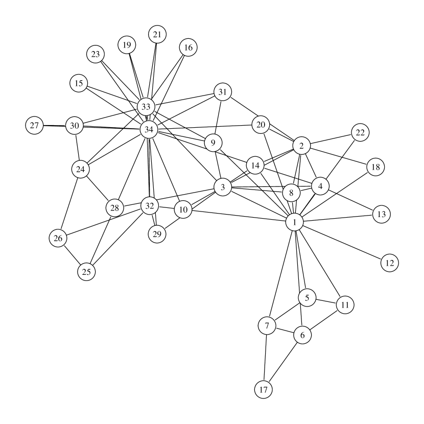
Figure 1: Zachary’s Karate club social network

We study Zachary’s Karate club social network [54]. The graph represents the friendship social network between the 34 members of a Karate club at a US university in the 70s. The graph contains 78 unweighted edges (its global density, the fraction of connected pairs of nodes, is thus equal to 13.9 %) and is represented on Figure 1 obtained with the Fruchterman-Reingold force directed algorithm [15] as implemented in igraph [8]. The transitivity of the graph, that is a measure of the probability that the adjacent vertices of a vertex are connected (see e.g., [51]), is equal to 25.6 %. The gap between the global density and the transitivity is a good indication for a larger local density and thus a relevant clustering.

5.1 Modularity maximization

It is well known from previous work on this graph that in terms of modularity, the optimal number of clusters is four (see e.g., [10]). This is a consequence of the structure of the modularity which tends to peak at a certain graph specific number of clusters and then decreases (this is another manifestation of the limited resolution of this measure [13]). For this graph, the social analysis conducted by Zachary leads to the definition of two clusters which correspond to the split between members of the club during the course of the study. Both clusters are split into two sub-clusters by modularity maximization (one ground truth cluster corresponds to clusters 1 and 4 in Figure 6 and the other to clusters 2 and 3). We have investigated the behavior of the deterministic annealing algorithm with $C$ ranging from $2$ to $8$. The parameters of the algorithm were the following ones: $\alpha=1.1$, $\gamma$ is chosen so that the final temperature is $T_{0}/10$ and $L=151$ (this relatively large value was used to obtained a convergence for each EM-like phase; a faster annealing introduced instabilities on this graph).

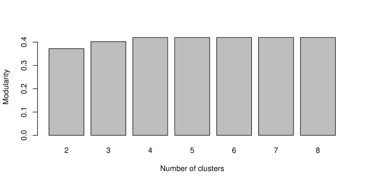
Figure 2: Maximal modularity achieved by DA as a function of $C$

Figure 3: Evolution of the modularity during annealing (the solid line corresponds to the theoretical temperature for the first phase transitions, dashed lines correspond to detected transitions)

As shown on Figure 2, the maximal modularity achieved by deterministic annealing (without a prior structure) reaches its maximum at $C=4$ clusters and then remains constant (the value of the maximum is $0.4198$, as reported in e.g., [10]). This is an interesting feature of DA: the algorithm is able to produce empty clusters if this increases the objective function. In the present case, the algorithm produces a maximum of four non empty clusters, even if we ask for eight. While this is interesting in terms of maximizing the modularity, this tends to increase the resolution problems faced by this quality measure [13]. The fuzzy layout strategy proposed in Section 4.2 is therefore expected to be very useful in this context.

Figure 3 shows the evolution of the modularity during annealing for the case $C=4$. More precisely, we compute the expectation of the modularity with respect to the mean field distribution:

$$\mathbb{E}_{R}\left(Q(M)\right)=\sum_{i\neq j}\sum_{k}\mathbb{E}_{R}\left(M_{ik}\right)\mathbb{E}_{R}\left(M_{jk}\right)B_{ij}+\frac{1}{2m}\sum_{i}\left(W_{ii}-P_{ii}\right)$$ (15)

The critical temperature appears, as expected, as a very conservative estimate of the temperature of the first phase transition. This first phase transition corresponds to the detection of two well identified clusters (the ones discovered by Zachary in [54]), while the second phase transition introduces two additional clusters. The evolution of the expectation of the assignment matrix $\mathbb{E}_{R}\left(M\right)$ is represented by Figures 4 and 5: each figure includes four copies of the graph. In copy number $k$, the gray level of the node $i$ encodes the value of $\mathbb{E}_{R}\left(M_{ik}\right)$, i.e., of the probability for node $i$ to belong to cluster $k$ according to the approximating distribution $R$.

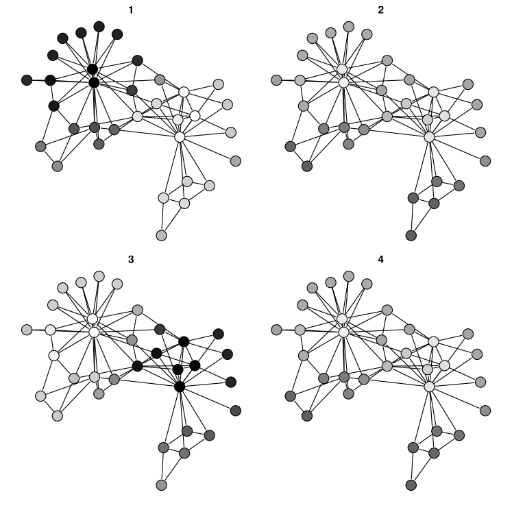
Figure 4: Assignment probabilities after the first phase transition: black corresponds to probabilities close to one, white to probabilities close to zero

After the first phase transition, clusters 1 and 3 start to take (partial) ownership of some of the vertices (the black ones on Figure 4), even if only 6 vertices out of 34 have a maximal assignment probability higher than 0.75. More than 40% of the vertices (14 out of 34) have rather fuzzy assignment probabilities (i.e., less than 0.5 for the maximal value).

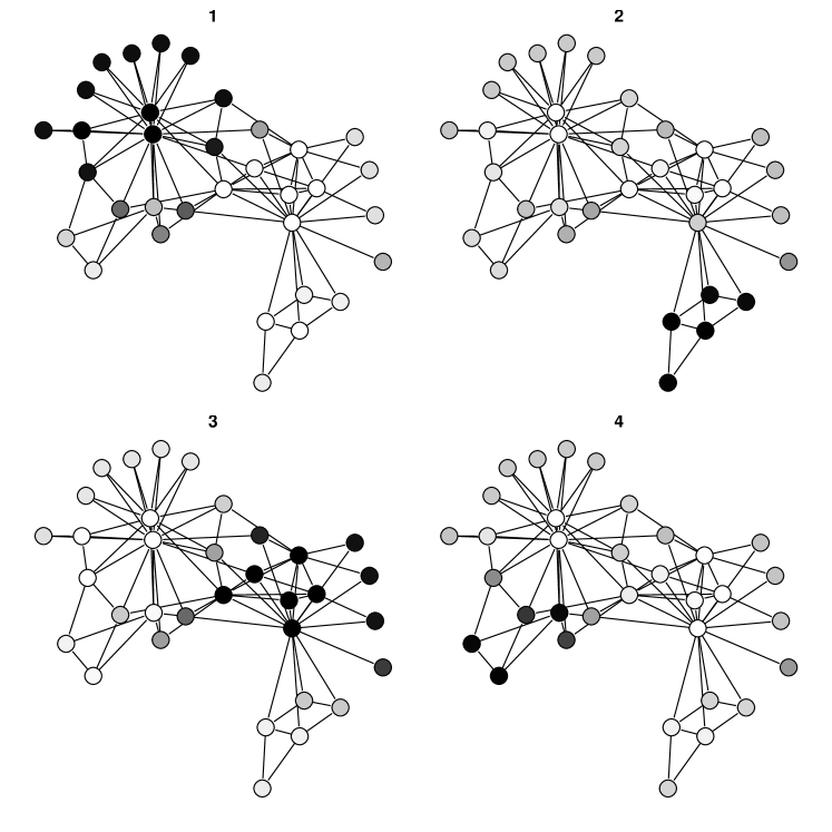
Figure 5: Assignment probabilities after the second phase transition: black corresponds to probabilities close to one, white to probabilities close to zero

After the second phase transition (shown on Figure 5), the algorithm has identified four distinct clusters accounting for 23 vertices (which are all assignments to a cluster with more than 0.75 probability). Four vertices still have a maximal assignment probability below 0.5. If the annealing is brought to the limit of a very low temperature (below the threshold of $T_{0}/10$ chosen here), the expectation of the assignment matrix is almost a 0/1 matrix, but such effort is not needed: in the case of the Karate club graph, all vertices have a maximal assignment probability higher than 0.5 at $T=T_{0}/10$ and a winner-take-all approach leads to a well defined clustering of the graph.

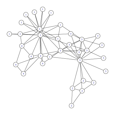
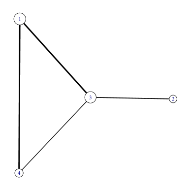
Figure 6: Left: original layout numbered according to the clustering; right: clustering induced graph

Figure 6 compares the original layout numbered via the clustering to the layout of the clustering induced graph (obtained by the Fruchterman-Reingold force directed algorithm [15]). The induced graph emphasizes clearly the relation between the clusters: cluster 2 is not directly connected to clusters 1 and 4, while the connection between 3 and 4 is less dense than the ones between 1 and 3 or 4. The summary is therefore quite informative, even if, as expected, most of the structure is lost. For instance, cluster 1 exhibits a start shape which is of course lost in the glyph based representation.

5.2 Organized modularity maximization

For the organized modularity, we use the simplest setting compatible with the four clusters identified in the previous section: the prior structure consists in a square in which each vertex is associated to a cluster. We use the following influence matrix:

$$S=\left(\begin{array}[]{cccc}1&\lambda&\lambda&0\\ \lambda&1&0&\lambda\\ \lambda&0&1&\lambda\\ 0&\lambda&\lambda&0\\ \end{array}\right),$$

where $\lambda$ specifies the amount of local influence (there is no diagonal influence). Interestingly, the value of $\lambda$ has an impact on the number of non empty clusters obtained by deterministic annealing. We use the same parameters for the algorithm as in the previous section, while varying $\lambda$ between $0$ and $0.2$. As shown on Figure 7, a large influence tends to reduce the number of effective clusters produced by the algorithm.

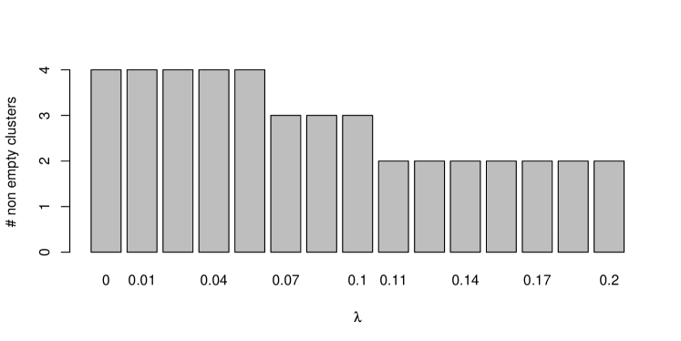
Figure 7: Number of non empty clusters as a function of the influence parameter $\lambda$

This can be explained by an analysis of the optimal four clusters clustering obtained before. As shown on Figure 6, there is no direct connection between cluster 2 and clusters 1 and 4. As a consequence, the corresponding entries $B_{ij}$ are negative: the only way to prevent the organized modularity to be smaller than the standard one is to put cluster 2 far away from clusters 1 and 4 in the prior structure. This is not strictly feasible as there are only two pairs of cluster positions with no direct influence in $S$ (they corresponds to the diagonal of the square). As a consequence, one might put cluster 1 far away from cluster 1 or from cluster 4, but not from both. Therefore, the modularity will decrease by e.g.,

$$-\frac{1}{2m}\sum_{i\in C_{2},j\in C_{4}}\lambda P_{ij},$$

if cluster $2$ has no influence on cluster $1$. Then, when $\lambda$ is large enough, the reduction of the four clusters organized modularity will be high enough to bring its value below the one of the two or three clusters standard modularity. Those latter configurations are easier to arrange on the prior structure in a way that minimizes negative contributions: they will be preferred by the algorithm over the four clusters solution.

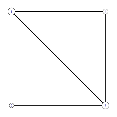
Figure 8: clustering induced graph displayed on the prior structure

In fact, the behavior of the algorithm is comparable to the one of a force directed method: when there is no connection between two vertices, they only repel each other and the algorithm tries to maximize their distances. As shown on Figure 8, the representation of the graph obtained via the prior structure is quite similar to the one provide by Figure 6. The underlying clusters are completely identical and thus use the same numbering to ease comparison between the figures (this is also the case when the value of $\lambda$ induces a clustering with two or three clusters: the obtained clusterings are the ones that maximize the standard modularity for $C=2$ or $C=3$).

5.3 Fuzzy layout

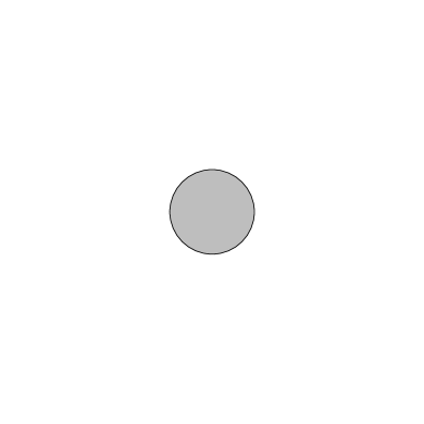
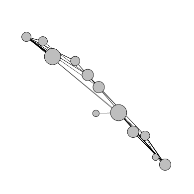
initial layout	after first phase transition
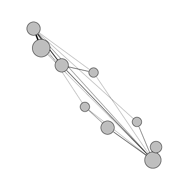
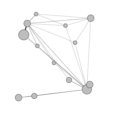
just before second phase transition	just after second phase transition
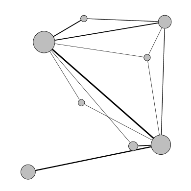
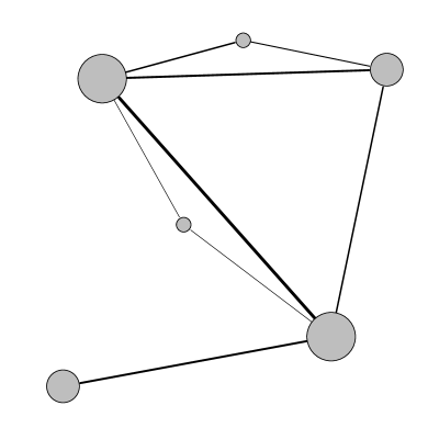
during the final cooling phase	final configuration

Figure 9: Evolution of the fuzzy layout during annealing (the Fruchterman-Reingold algorithm was used to reduce edge overlapping)

It might seem from Figure 8 and more generally from the discussion above that the organized modularity offers no particular interest compared to a two phases approach with a maximal modularity clustering followed by a force directed layout. The behavior of the DA algorithm on the Karate graph emphasizes the fact that the modularity does not increase with the number of clusters: it tends to peak at an optimal graph specific number. As explained before, there is a complex interaction between the prior structure and the values of the modularity for different numbers of non empty clusters. In some situations, the prior structure introduces a too strong coupling between clusters and leads this way to a reduced number of non empty clusters. This might lead to a better visualization of the graph, to an over simplification or to nothing more than the two phases approach (Section 6 will illustrate this further).

The first way to address this problem is to test several prior structures and to select optimal graphs with respect to different quality measures as proposed in Section 4. A second (and complementary) approach consists in leveraging the annealing process to limit the impact of the peaking behavior of the modularity by means of the fuzzy layout strategy described in Section 4.2. An example of such layouts is given by Figure 9. The representations give a more complete picture of the graph than Figure 6 (or Figure 8). It appears for instance quite clearly that two vertices are not easy to assign to the final four clusters (they are at the boundary of cluster 1 in Figure 8). If we study carefully the original representation on Figure 1 with the added knowledge provided by Figures 6 and 9, those vertices (number 10 and 24) appear quite clearly in between two clusters. However, it would be almost impossible to obtain this information directly from the original representation. Figure 9 shows also that the composition of cluster 3 (in Figure 8, bottom left in Figure 9) is quite obvious compared to others. This is easily confirmed on Figure 6.

5.4 Comparison with SOM variants

As the proposed method is based on the SOM rationale, it seems natural to compare it to SOM variants that can handle graph nodes, mainly the kernel SOM with adapted kernels [47] and the spectral SOM [48]. Details on those methods and on parameters optimization are postponed to Section 6.2 in order to keep the present Section focused on a detailed analysis of the Karate graph.

Following the methodology described in Section 6.2, we have built Pareto optimal points with respect to the modularity of the clustering and the number of edge crossings in the induced layout. The only global Pareto optimal point among SOM variants has been obtained by the heat kernel (see [27]). It has zero edge crossing and a modularity of 0.4188. The obtained layout is identical to one of Figure 8, up to a rotation. However, the underlying clustering is slightly different, as shown by the reduced modularity. In fact, node number 10 on Figure 1 is assigned to the same cluster as node number 3 rather than to node number 34’s cluster in the optimal clustering (in terms of modularity). It turns out that node number 10 should be assigned to node number 34’s cluster according to Zachary’s analysis. Therefore, the best SOM variant fails to recover exactly the ground truth clustering, while modularity optimization does recover a finer clustering.

Other variants make similar or worse mistakes. For instance, the best result obtained by the modularity kernel SOM has a modularity of 0.409 which corresponds to two differences with the optimal modularity clustering. Node number 10 is misclassified compared to Zachery’s two clusters ground truth, while node number 24 is assigned to the correct Zachery’s cluster but to a different cluster than in the highest modularity clustering.

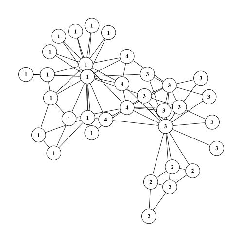
Figure 10: Original layout numbered according to the clustering obtained by the Laplacian’s inverse kernel SOM

The best solution for the Laplacian’s inverse kernel SOM has an even worse modularity of 0.391. In this case, the differences between the proposed clustering and the ground truth are more important. Figure 10 gives the clustering obtained by the Laplacian’s inverse kernel SOM on the full layout of the Karate graph. Node number 3 is assigned to a wrong cluster according to the ground truth. While the mismatch corresponds to only one node, the status of this node is much more obvious than the one of node 10: it is connected to node number 1, the central actor one of the clusters identified sociologically. In addition, cluster number 4 seems to consist in boundary nodes rather than in a dense subset of nodes. While this SOM variant manages to reach a fair approximation of the ground truth clustering, it splits one of those clusters in a misleading way: cluster 4 is not dense and its members are more connected to outside nodes than between themselves.

In summary, the SOM variants are unable to recover exactly the ground truth clustering obtained by Zachary on this graph. In addition, the SOMs give an example of a clustering with reduced modularity (compared to optimal ones) with a possibly misleading cluster: the subgraph is not dense and nodes have more connections outside of the cluster than inside. Limitations of graph SOMs compared to our proposal will be confirmed in the next Section.

6 Results on larger graphs

6.1 Datasets

In order to confirm the conclusions reached in the previous section, the following experiments provide a comparison between the proposed method, the classical two phases approach and SOM variants on three larger graphs. More precisely, the studied graphs are:

• a coappearance network of characters in chapters of the novel Les Misérables (Victor Hugo), introduced by [25] and available at http://www-personal.umich.edu/~mejn/netdata/lesmis.zip. This graph is undirected and weighted by the number of chapters in which each pair of characters appear together. It is larger than the graph described in Section 5 with 77 nodes representing the characters of the novel. The global density of this graph is equal to 8.7% and its transitivity is equal to 49.9%. This indicates that the local connectivity of the graph is very high compared to its global one and thus that this graph is likely to be clustered into dense subgroups. This graph is represented in Figure 11 (this layout has been obtained via the Fruchterman-Reingold force directed algorithm [15] as implemented in igraph);

• a directed, weighted network representing the neural network of the worm “C. Elegans”, introduced by [52] and available at http://cdg.columbia.edu/cdg/datasets. The graph has been used as an undirected weighted graph: the weights, $(W_{ij})$, of the undirected graph are simply defined from the weights $(\overrightarrow{W}_{ij})$ of the directed graph by $W_{ij}=W_{ji}=\overrightarrow{W}_{ij}+\overrightarrow{W}_{ji}$. This graph is connected and contains 453 nodes. Its density is equal to 2.0% and its transitivity to 12.4%. Compared to the graph from “Les Misérables”, this network has a much smaller local connectivity indicating that the clustering task should be harder. Hence, a smaller modularity is expected for the resulting clustering. This graph is represented in Figure 12 (left). While the graph from “Les Misérables” was readable, the “C. Elegans” graph is impossible to decipher when rendered by the standard Fruchterman-Reingold algorithm;

• a network representing the e-mail exchanges between members of the University Rovira i Virgili (Tarragona), introduced by [19] and available at http://deim.urv.cat/~aarenas/data/xarxes/email.zip. This graph is also connected and contains 1 133 nodes. Its global density is equal to 0.9% and its transitivity to 16.6%. As in the previous case, the transitivity of the graph is not very high but the gap between the global density and the transitivity is much larger and a larger modularity than for “C. Elegans” can then be expected. This graph is represented in Figure 12 (right) and is as undecipherable as the “C. Elegans” one when rendered with the Fruchterman-Reingold algorithm.

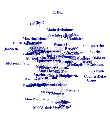
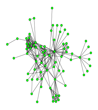
Figure 11: Coappearance network from “Les Misérables” (left: with characters’ names; right: without label)

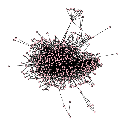
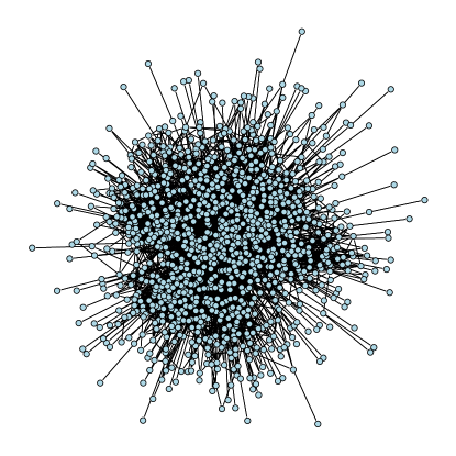
Figure 12: Two real-world networks: Neural network of the worm C. Elegans (left) and E-mail network between the members of the University Rovira i Virgili (right)

6.2 Experimental setting

6.2.1 Reference methods

The experiments compare the proposed method with two other approaches:

1. as explained in Section 2, the proposed approach tries to improve the standard two phases approach by building topographically ordered clusters. The reference approach consists therefore in a two phases method already used in Section 5.1: we build a good clustering via deterministic annealing maximization of the modularity and the graph induced by the clustering is rendered via a force directed placement algorithm (the Fruchterman-Reingold algorithm as implemented in igraph);

2. an alternative organized approach is the one described in [47]: Kohonen’s Self Organizing Map algorithm is used to build a topographically ordered clustering of the graph (on a prior grid) via a well chosen graph kernel. Several popular kernels are defined for graphs, including regularized versions of the Laplacian (see, e.g., [44]), the generalized inverse of the Laplacian [14] or the modularity kernel [55]. The latter one is defined from the positive part of the matrix $B$ involved in the definition of the modularity (see equation (5)).

   A slightly different way to use the Self Organizing Map for clustering the vertices of a graph is what is called “spectral SOM” in [48]. This approach is inspired by spectral clustering (see e.g., [49]) but using a SOM instead of the usual $k$-means algorithm. More precisely, the vertices of the graph are represented by vectors of $\mathbb{R}^{C}$ (where $C$ is the initial number of clusters of the prior grid) that are the coordinates of the eigenvectors associated to the $C$ smallest non zero eigenvalues of the Laplacian of the graph. Then, a usual vector SOM is applied to these vectors.

   Those four SOM variants were used in Section 5.4 for the Karate graph.

6.2.2 Parameters optimization

The parameters optimization procedure outlined in Section 4.1 is applied to tunable parameters of the reference methods (e.g., the number of clusters, the kernel and its parameters, etc.). Random initialization is included in the procedure for methods that are not deterministic.

In the specific case of the two phases approach, we rely on a two phases optimization: the best clustering is selected by maximization of the modularity over the number of clusters and then the layout with the lowest number of crossing edges is kept among 10 different random initializations for the Fruchterman-Reingold algorithm.

The other solutions are “all-in-one” and provide at the same time a clustering and a layout. We select therefore on Pareto optimal parameter sets. The following parameters were optimized:

• the number of clusters for the clustering algorithm was optimally chosen in $\{2,\ldots,25\}$ (please note that all methods can produce empty clusters);

• the prior structure was encoded via a square grid selected among 3 sizes: $3\times 3$, $4\times 4$ and $5\times 5$ (i.e., 9 clusters, 16 clusters and 25 clusters). The vertices of the grid have integer coordinates;

• the entries of the matrix $S$ were calculated via equation (13). We compared exponential decrease and linear decrease, and used at least four different scaling values, chosen according to the induced radius of influence in the prior structure;

• in the case of the SOM (kernel version or “spectral SOM”), the optimal configuration (size of the prior structure and neighborhood function) was selected in the same set of configurations as for the organized modularity;

• as the batch SOM used in this paper exhibits some dependence to the initial configuration, we used 5 different initializations for each run of the algorithm. Among them 4 were random ones and the last one was a PCA based initialization in which the prior structure is positioned on the plane spanned by the first two principal components (this is done with kernel PCA [43] in the case of kernel SOM and standard PCA in $\mathbb{R}^{C}$ for the spectral SOM);

• as explained above, we used three different kernels. Among them, only the heat kernel has a parameter: it is defined as $K=e^{\beta L}$ where $L$ is the Laplacian of the graph and $\beta$ a temperature parameter. Four values of $\beta$ were used;

  We used the three kernels only for the analysis of “Karate” and “Les Misérables”. For the two other graphs (C. Elegans and E-mail), we restricted the analysis to the generalized inverse that has achieved almost the best results in the first experiment (comparable with the best ones obtained for the heat kernel) and that does not require the tuning of an additional parameter.

6.3 Results and comments

6.3.1 Numerical results

We first compare the proposed method to the SOM variants with respect to the chosen quality criteria: the modularity of the clustering and number of edge crossings in the associated representation. As explained in Section 2 and 4.1, those quality criteria have been chosen in order to obtain a good compromise between a readable clustering based representation of the graph (with small number of edges crossing) and the fairness of this representation (dense clusters, i.e., high modularity). Figures 13 and 14 give the values of the quality criteria for all the experiments made on the dataset “Les Misérables”, while Tables 1, 2 and 3 give the pairs of values associated to Pareto points obtained in for each graph. We first focus on “Les Misérables” and then give more general comments. Please note that comments and conclusions about “Les Misérables” apply to the Karate graph with the only exception that the modularity kernel SOM performs in an acceptable way on the Karate graph. Detailed results are not included to avoid lengthening the article.

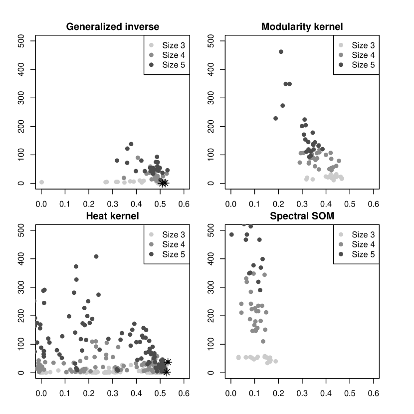
Figure 13: Quality criteria for the kernel and spectral SOM for “Les Misérables”: $x$ axis is the modularity and $y$ axis is the number of edge crossings. The gray level of the points gives the initial size of the square grid and Pareto points are indicated by a black star. Solutions with a modularity lower than 0 or a number of edge crossings greater than 500 are omitted on this figure.

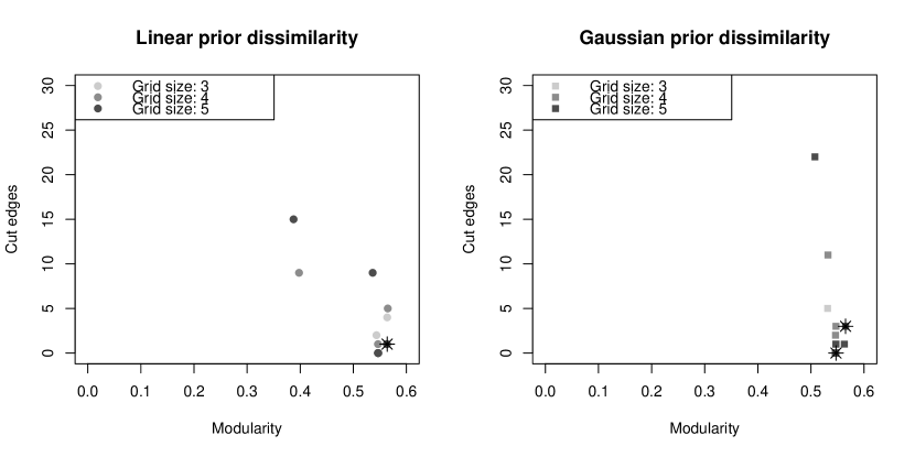
Figure 14: Quality criteria for the optimization of the organized modularity by deterministic annealing for “Les Misérables”. The gray level of the points gives the initial size of the square grid and Pareto points are indicated by a black star.

As shown in Figures 13 and 14, the clusterings obtained on “Les Misérables” by optimizing the soft modularity have generally larger modularity values than those produced by SOM variants. In addition, only a limited subset of the parameter space leads to high modularity with SOM variants. Both outcomes were expected for kernel SOMs using the heat kernel and the generalized inverse of the Laplacian. Indeed those kernels induce feature spaces and associated clustering objectives that have no simple relation with the modularity criterion. As shown in e.g. [4, 53] both kernels lead to interesting clustering results, but it is clear from the present results that one cannot expect to get high modularity clustering from them in general.

The poor results for the spectral SOM are slightly less expected as this method is related to some form of graph cut measure optimization, using the relaxation proposed in spectral clustering [49]. However, as recalled in Section 2.2, graph cut measures are quite different from the modularity, which probably explains the low modularity clusterings obtained by this method.

Finally, the results obtained by the modularity kernel are quite disappointing. Indeed, this kernel is strongly related to the modularity measure [55] and should lead to some form of modularity maximization. In practice, it seems that taking only the positive part of the $B$ matrix does not capture all the complexity of the modularity, at least in the SOM context.

Of course, as our method aims at maximizing an organized version of the modularity, the higher quality of the results in terms of a closely related measure (the classical modularity) is rather natural. However, the Figures show that it also leads to a low number of edge crossings and therefore to more readable layouts. Figure 13 shows in particular that SOM variants generally fail to balance modularity and edge crossings: high modularity clusterings have frequently a significant number of edge crossings (see also Table 1).

Les Misérables
Method	Number	Modularity	Nb of pairs	Id
	of clusters		of cut edges
SOM (heat kernel)	$5^{2}$ (22)	0.5327	37	M1
	$3^{2}$ (8)	0.5276	2	M2
SOM (Laplacian’s inverse)	$3^{2}$ (9)	0.5212	1	M3
	$3^{2}$ (8)	0.5089	0	M4
Organized mod. (linear)	$4^{2}$ (7)	0.5638	1	M5
Organized mod. (Gaussian)	$5^{2}$ (7)	0.5652	3	M6
	$3^{2}$ (6)	0.5472	0	M7
Modularity optimization	8 (5)	0.5472	0	M8

Table 1: Description of the Pareto points for each of the three methods (SOM, optimization of organized modularity and optimization of ordinary modularity) applied to the dataset “Les Misérables”. The number of clusters gives the number of clusters $C$ used by the algorithm and, in parenthesis, the number of non empty clusters obtained finally. The column “Id” is used to identify the corresponding solution in the text; Pareto points within all solutions have bold Id.

Combining both criteria lead to the search of Pareto points. The case of “Les Misérables” is summarized by Table 1: when considered all together, the SOM approaches (kernels and spectral) lead to 4 Pareto points which are of lesser quality than the one obtained by the proposed approach: none of the Pareto points for kernel SOM is a global Pareto point for the dataset mainly because of low modularity values. In addition, and for similar reasons, the spectral SOM and the modularity kernel SOM do not produce any Pareto point. In fact, the only realistic competitive method in the SOM family is the kernel SOM based on Laplacian’s inverse. Indeed, it gives comparable results as the ones obtained with the heat kernel but without the need for a time consuming kernel parameter tuning. The two larger datasets, “C. Elegans” and “E-mail” were therefore investigated only with this kernel SOM, excluding all other variants. Pareto points are described in Tables 2 and 3.

C. Elegans
Method	Number	Modularity	Nb of pairs	Id
	of clusters		of cut edges
SOM (Laplacian’s inverse)	$3^{2}$ (9)	0.3228	14	CE1
	$3^{2}$ (9)	0.3000	7	CE2
	$3^{2}$ (8)	0.2936	1	CE3
Organized mod. (linear)	$4^{2}$ (8)	0.4373	41	CE4
	$3^{2}$ (7)	0.4348	27	CE5
	$3^{2}$ (7)	0.4321	19	CE6
Organized mod. (Gaussian)	$3^{2}$ (8)	0.4063	15	CE7
Modularity optimization	18 (8)	0.4383	27	CE8

Table 2: Description of the Pareto points for each of the three methods (SOM, optimization of organized modularity and optimization of ordinary modularity) applied to the dataset “C. Elegans”. The number of clusters gives the number of clusters $C$ used by the algorithm and, in parenthesis, the number of non empty clusters obtained finally. The column “Id” is used to identify the corresponding solution in the text; Pareto points within all solutions have bold Id.

Results from “C. Elegans” and “E-mail” generally agree with those obtained on “Les Misérables”: the kernel SOM does not produce clusterings with high modularity, but it manages sometimes to reach a low number of edge intersections in the induced layout. That said, the kernel SOM does not produce global Pareto points for “Les Misérables” and “E-mail”: on those datasets, it is therefore strictly less efficient than the proposed method on the dual objectives point of view (this was also the case for the Karate graph). The best situation for the kernel SOM is “C. Elegans” where the very low numbers of edge crossings of configurations CE1, CE2 and CE3 make them Pareto points within the full set of solutions. However, those points have very low modularities compared to other solutions.

E-mail
Method	Number	Modularity	Nb of pairs	Id
	of clusters		of cut edges
SOM (Laplacian’s inverse)	$4^{2}$ (16)	0.4652	218	E1
	$3^{2}$ (9)	0.4566	49	E2
	$3^{2}$ (9)	0.4540	24	E3
	$3^{2}$ (9)	0.4420	22	E4
	$3^{2}$ (9)	0.4242	19	E5
Organized mod. (Gaussian)	$3^{2}$ (8)	0.5694	47	E6
	$4^{2}$ (8)	0.5693	44	E7
	$4^{2}$ (7)	0.5554	25	E8
	$3^{2}$ (7)	0.5456	23	E9
	$5^{2}$ (6)	0.5401	11	E10
Modularity optimization	11 (8)	0.5736	56	E11

Table 3: Description of the Pareto points for each of the three methods (SOM, optimization of organized modularity and optimization of ordinary modularity) applied to the dataset “E-mail”. 11 Pareto points have been found for the kernel SOM but 6 of them are omitted in the table because of a very low modularity (less than 0.2). The number of clusters gives the number of clusters $C$ used by the algorithm and, in parenthesis, the number of non empty clusters obtained finally. The column “Id” is used to identify the corresponding solution in the text; Pareto points within solutions have bold Id.

In summary, those experiments show that the spectral SOM and the modularity kernel SOM should be avoided as they cannot produce satisfactory results in terms of the chosen quality criteria. In addition, while the heat kernel can produce interesting results, its additional kernel parameter induces a large computational cost: as shown on Figure 13 most of the computing efforts are wasted as they lead to poor solutions on both criteria. The only competitive method is the Laplacian’s inverse kernel SOM. But even if it seems to be the best SOM based method, it still produces sub-optimal solutions on both criteria for three out of four datasets.

The comparison between the classical two phases approach and our method does not lead to a clear winner as far as the chosen quality criteria are concerned. As expected, the modularities of the clusterings obtained in the two phases approach are among the highest. Interestingly, maximizing the organized modularity can lead to a higher modularity than a more direct approach (in a similar way as the SOM which can overcome the $k$-means in term of within cluster variance): this is the case for “Les Misérables” (see Table 1). However, in general, the two phases approach gives the clusterings with the highest modularity. In term of edge crossings, the two phases approach gives also satisfactory results: this confirms the analysis from Section 2.2, where we argued that looking for dense clusters should reduce the number of edges between clusters. On complex graphs however, our method leads to lower numbers of edges cuts: again, this confirms the somewhat contradictory nature of the two quality criteria explained in Section 2.2.

By construction, the two phases approach should give a Pareto optimal result, up to sub-optimal optimization results caused by the combinatorial nature of both optimization problems. In practice, we obtained Pareto points on all graphs. In general, those points have higher modularity and higher number of edge crossings than the ones produced by our method, as expected: our clusters are somewhat adapted to the clustering induced layout. There is therefore no obvious superiority of one method over the other. In fact, we are more interested in the final layout of the graphs than in the exact numerical results. It is therefore interesting to study the visual representations obtained different approaches, as long as they correspond to Pareto optimal points. This is done in the next subsection.

6.3.2 Drawing the graph from its clustering

The aim of the proposed method is to provide a simplified but relevant representation of a large graph through the graph induced by the clustering. The present section analyses the visual representation obtained via the proposed method and reference methods. We first start with a detailed analysis of “Les Misérables”: Figure 15 gives the representation of the graph of clusters for clusterings M5 and M8 (See Table 1).

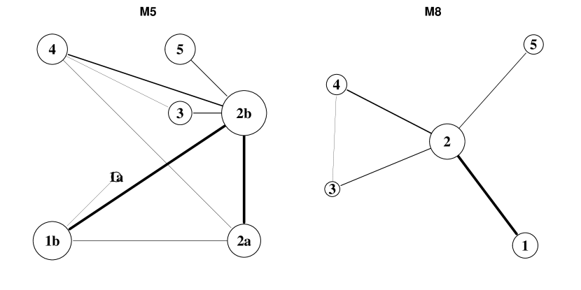
Figure 15: Clustering induced graphs. Left: displayed on the prior structure (for M5 obtained by optimizing the organized modularity) and Right: displayed by Fruchterman and Reingold algorithm (for M8 obtained by optimizing the ordinary modularity).

As the graph is small enough, those layouts can be compared to the original layout numbered according to the clustering: this is provided by Figure 16.

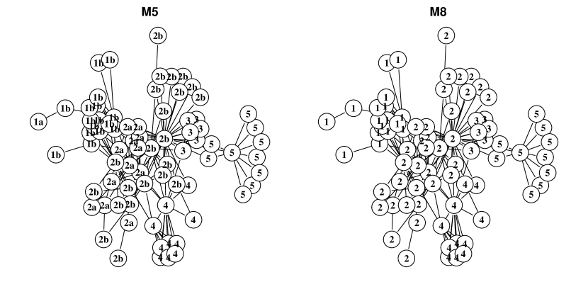
Figure 16: Original layout of “Les Misérables” labeled according to the clustering; left: M5 (optimization of the organized modularity) and right: M8 (optimization of the ordinary modularity). The number on the vertices is the cluster’s number.

The density of the graph limits the possibilities of analysis, but it appears clearly that cluster 1a from M5 corresponds to a quite isolated character (Mother Plutarch who is only connected to Mabeuf), while up to a single character (Sister Simplice), the union of clusters 2a and 2b in M5 gives cluster 2 in M8. In both cases, the summary of the graph given by the clustering seems therefore reasonable and a more detailed analysis is needed.

It turns out that both representations give a clear understanding of the story of the novel. It is based on a central group of characters (clusters 2a and 2b for M5 and 2 for M8) which includes Valjean, Cosette and Marius (among others). Several sub-stories are narrated in the novel: the story of the Bishop Myriel who is spiritual guide of Valjean (clusters 5); the story of the street children Gavroche (clusters 1 in M5 and 1b in M8); and finally the story of Fantine, poor Cosette’s mother (clusters 4). But representation M5 gives another information by separating the main characters into the ones related to Valjean (Cosette, Marius, Javert, etc. in cluster 2b) and the ones related to the Thénardier family (mister and misses Thénardier, Éponine, their daughter, etc. in cluster 2a). In addition, cluster 2b of M5 (the main characters) has more connections to cluster 1b than cluster 2a (Thenardier family) to cluster 1b. Therefore, the central position of cluster 2b remains clearly emphasized in M5, even if the representation is arguably slightly less readable than representation M8 (it should be noted that the graph induced by the clustering M5 is planar, but because the organized layout is not optimized by a graph drawing algorithm, the actual representation has one edge crossing). Hence, with a small (and avoidable) increase in the number of edge crossings but with a higher quality of clustering, the information given by clustering M5 provides a more complete picture of the original network.

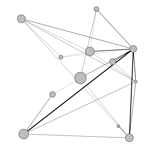
Figure 17: Fuzzy layout of the final configuration of “Les Misérables” (the Fruchterman-Reingold algorithm was used to reduce edge overlapping)

Additional insights can be gained with the help of the fuzzy layout methodology described in Section 4.2. Figure 17 gives an example of such layout for the final configuration of the deterministic annealing. At first, this representation might seem very different from M5 on Figure 15. In fact most of the differences can be explained by two phenomenons. Firstly, as on Figure 9 for the Karate graph, some nodes are difficult to assign to a given cluster and appear therefore in intermediate position. This explains the presence of some small clusters in between larger ones : this is the case, for example, of the small cluster at the extreme right of the Figure who is Javert, the policeman who is pursuing Valjean (one of the character of the larger cluster just above the small isolated one). But this character is also very related to the Thénardiers’ family (larger cluster below the small isolated one) because they capture and imprison him at the end of the novel. The small cluster situated between the large central cluster and the cluster at the bottom left part of the map is also interesting. It contains 3 characters that act as connections between several secondary characters and the rest of the graph: these characters belong to cluster number 5 in clusterings M5 and M8.

The second source of differences between M5 and the fuzzy layout is that several characters are extremely difficult to assign to a cluster and have therefore almost flat assignment probabilities $\mathbb{E}_{R}\left(M_{ik}\right)$ even at low temperature. Then, the corresponding nodes assume an almost barycentric position in the fuzzy layout: this explains the presence of a central node in Figure 17. The characters assigned to this central node are not connected and this cluster should not be seen as a meaningful one. On the contrary, it contains very isolated characters who belong to clusters 5, 2 or even 1 in clustering M8. All these characters have in common to share only a (small weighted) connection with another character of the network. They are very secondary characters in the novel. None of those ambiguities could have been detected on a standard two phases approach or on the SOM variants.

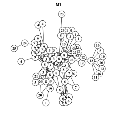
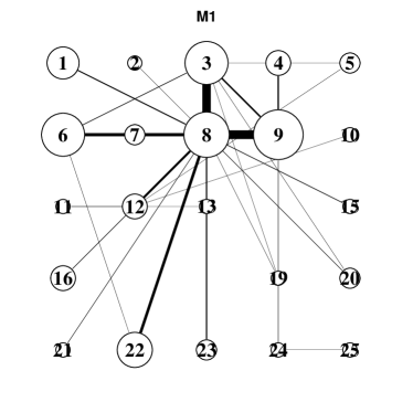
Figure 18: Representation of the M1 clustering obtained with the heat kernel SOM on the original layout (left) and via the prior structure (right)

In addition, the SOM variants obtain poor results on this graph. As shown in Table 1 they do not provide any global Pareto optimal points. Therefore it is not very surprising to obtain unsatisfactory visual representations from those methods. Figure 18 represents the results associated to clustering M1 in Table 1 (obtained with the heat kernel SOM). The resulting clustering has numerous non empty clusters and leads to a quite cluttered visual representation. In addition, some clusters seems completely arbitrary: for instance clusters number 5, 10, 11, 13 and 16 are a seemingly random clustering of the characters related only to the Myriel characters. The global impression is that the heat kernel SOM suffers from a tendency to build too fine clusterings on a somewhat arbitrary basis.

Figure 19: Representation of the M4 clustering obtained with the Laplacian’s inverse kernel SOM on the original layout (left) and via the prior structure (right)

The cluster and layout obtained by the Laplacian’s inverse kernel SOM are given on Figure 19. Results are quite different from those of the heat kernel SOM. Indeed, the clustered layout is very easy to read as there are no edge crossing. However, the rather low modularity of M1 (see Table 1) is an indication that clusters are not as dense as for clusterings M5 and M8. In fact, the representation of M1 clustering on the original layout of the graph shows that the associated visualization is quite misleading. For instance, cluster 3 contains Mother Plutarch while its unique connection in the graph, Mabeuf, is in cluster 6. Therefore cluster 3 is not even connected. A similar problem can be seen in cluster 2. Then the main underlying assumption of the clustering induced layout is not fulfilled: some clusters are not dense at all and are then meaningless.

This thorough analysis of “Les Misérables” confirms results on the Karate graph (Section 5) and the numerical analysis from the previous section. The analysis leads to two important conclusions. Firstly, the relevance of modularity and of edge crossings is confirmed: the rather poor results obtained by SOM variants in terms of numerical results correspond either to layouts that are difficult to read (see Figure 18) and/or to misleading clustering (see Figures 18 and 19). Secondly, the proposed methodology leads to a better understanding of the graph than the two phases approach by means of different clusterings (induced by the organized modularity maximization) and via the fuzzy layout methodology.

The sizes of “C. Elegans” and “E-mail” graphs make them difficult to analyze in details. We provide therefore only some qualitative comparisons of the layouts obtained by the investigated methods.

Figure 20 gives four layouts of the graph “C. Elegans” obtained from a subset of Pareto points of Table 2:

• CE1 is the layout obtained by kernel SOM with the highest modularity (chosen to avoid misleading clusterings);

• the CE8 is the layout obtained by the two phases approach and is induced by the clustering with the highest modularity;

• CE6 and CE7 are the two Pareto points obtained by our method: CE7 has the smallest modularity but also a smaller number of edge crossings within this two solutions. These two solutions have a high modularity (larger than 0.4) and the modularity of CE6 is very close to those of CE8 but with a smaller number of edge crossings.

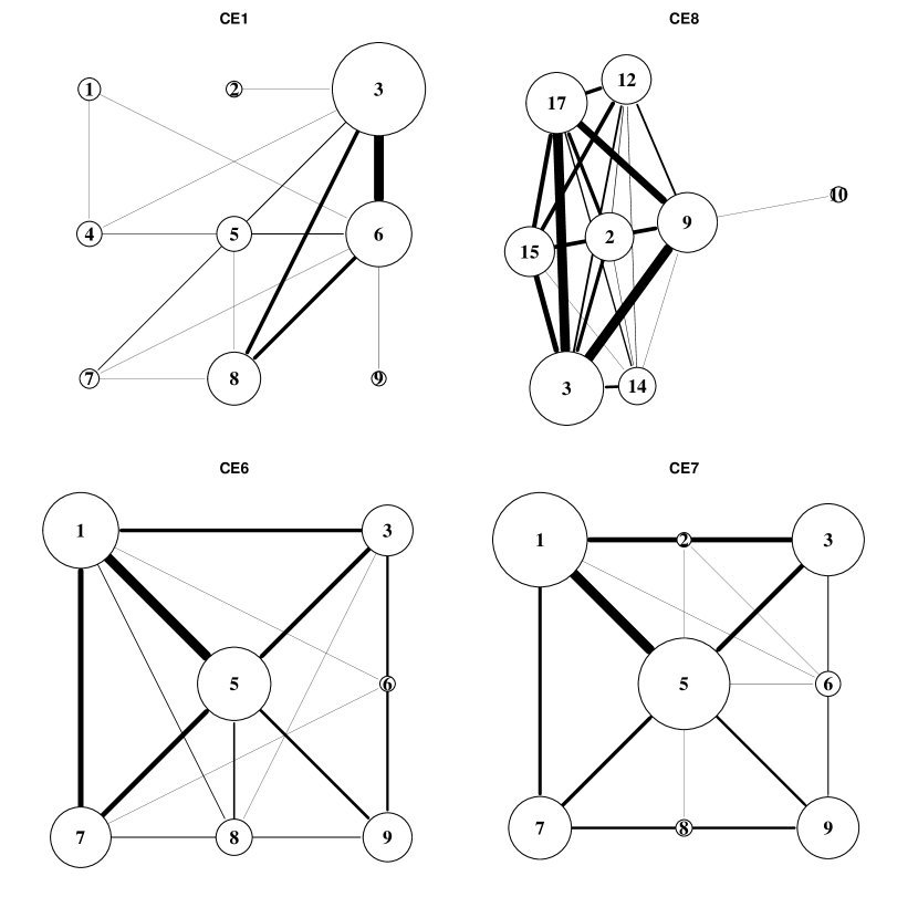
Figure 20: Clustering induced graphs for the “C. Elegans” dataset. Top left: displayed on the prior structure (for CE1 obtained by kernel SOM); Top right: displayed by Fruchterman and Reingold algorithm (for CE8 obtained by maximization of the modularity); Bottom: displayed on the prior structure (for CE6 and CE7 obtained by maximization of the organized modularity).

Despite a very small number of edge crossings, CE1 is poorly informative: three clusters (3, 6 and 8) contain more than 80 % of the vertices of the graph and the other clusters are thus very small compared to the three largest ones. The small clusters are then not very informative and their existence probably explains the poor modularity of the clustering. In fact, all solutions provided by kernel SOM for this dataset share the same problem with some large clusters and some very small ones. This type of behavior is neither specific to the chosen graph, nor to the Laplacian’s inverse kernel as shown on Figure 19 and in [4] for the heat kernel.

CE8 shows another type of layout problems: the graph induced by the clustering is almost a complete graph (up to cluster 10, the graph is complete). The only information conveyed by this layout is that nodes in cluster 10 are only connected to nodes in cluster 9. The width of the edges can be used to infer that some clusters are only loosely connected (e.g., 12 and 14), but grasping the general organization of the graph is quite difficult with this layout.

CE6 and CE7 both have a slightly smaller modularity than CE7 but they are easier to read because of a smaller number of edge crossings. Their clustering qualities are higher than the one of CE1 (with a modularity larger than 0.4 and less imbalance between the clusters’ sizes), comparable for CE6 to the one of the clustering obtained in the two phases method CE8. Therefore, CE6 (and to a lesser extent CE7) is almost as faithful as CE8 but gives some understanding of the structure of the graph because the resulting simplified graph is not complete. As expected, a small reduction in clustering quality can lead, in some situations, to clusters that are more adapted to visual exploration. This validates again the principle of integrating the clustering process and the layout process.

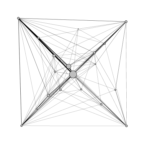
Figure 21: Fuzzy layout during the final cooling phase for the solution CE6 of “C. Elegans”

In addition, fuzzy layouts such as the one provided in Figure 21 can be used to analyze how clusters are built during annealing. In the particular case of solution CE6, the layout shows that, e.g., cluster 8 is formed at the end of the annealing. The analyst can investigate first the associated nodes and their connection pattern to outside clusters, or on the contrary, focus his/her attention on well established clusters.

Finally, Figure 22 provides two layouts of the graph “E-mail”. We chose to represent the solution obtained by the two phases approach (E11, see Table 3) and the Pareto point obtained by our method with the smallest number of edge crossings (E10).

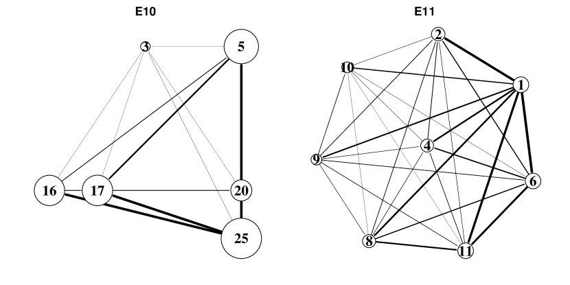
Figure 22: Clustering induced graphs for the “E-mail” dataset. Left: displayed on the prior structure (E10 obtained by maximization of the organized modularity); Right: displayed by Fruchterman and Reingold algorithm (E11 obtained by maximization of the modularity).

As in the previous example, the solution provided by the optimization of the organized modularity, despite a clustering quality that is slightly worse, gives a more understandable simplification of the graph than the dual phases approach. In fact, the graph associated to E11 is complete and one has to rely on the width of the edges to try to infer the importance of the relations between clusters. The layout associated to E10 seems therefore easier to grasp. In addition, the associated fuzzy layout (see Figure 23) shows that most of the clusters are well defined and identifies a few nodes that are difficult to assign to clusters. Further investigations could target those nodes.

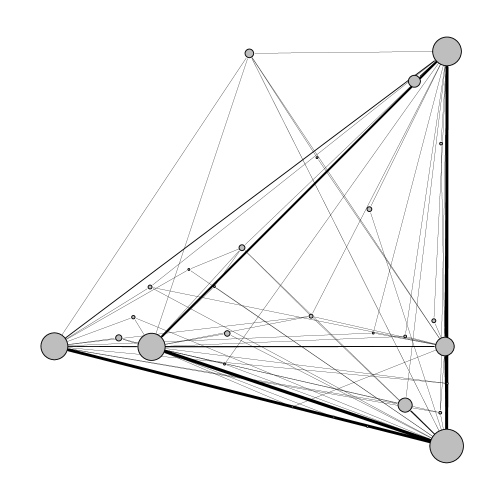
Figure 23: Fuzzy layout during the final cooling phase for the solution E10 of “E-mail”

6.3.3 A brief summary of the experiments

Several conclusions can be drawn from the experiments conducted on the four real world graphs. Firstly, maximizing the organized modularity leads to good solutions with a high modularity and a acceptable number of edge crossings. In some situations, maximizing the organized modularity actually gives a higher modularity clustering, in a similar way to what can be observed for the SOM versus the $k$-means. However, the main gain is a better trade off between modularity and readability of the clustering induced graph: we trade a small reduction in modularity for either a larger number of clusters (limiting the general tendency of the modularity to pick up a small number of clusters) or a reduced number of edge crossings (or both). All in one, organized modularity maximization brings therefore simplified representations of graphs that seem more informative than the standard two steps approach. In addition, as the modularity is almost optimal, the representations provided by maximization of the organized modularity are reasonably faithful, especially compared to the low quality results generally obtained by graph adapted SOM. While the final layout obtained by the organized modularity are not perfect (it is quite clear for instance that the left graph on Figure 15 is planar and could be rendered with no edge crossing), their ordered and regular nature makes them very readable. In conclusion, we consider that a good practice consists in combining our method to the two phases approach to get different and complementary views on the same graph. A future implementation challenge is to provide linked multi-views [1] of a graph that would give the analyst a visual comparison method between those views.

In addition, relying on deterministic annealing provides a path in the clustering space that is worth exploring via intermediate fuzzy layouts. The main advantage of those layouts is to increase the number of clusters and to providing hints on the final assignment of vertices. Atypical vertices are clearly pinpointed with this approach and can be further studied by the analyst. Our use of the fuzzy layout was quite limited in this paper as we believe they should be provided in an interactive environment in which the analyst can navigate in the algorithm results. Further studies are needed to validate the interest of the concept. In addition, as those layouts are closer to clustered layouts than the rest of our work, comparisons with those latter methods (e.g., [35]) would be interesting.

Those results show that the combination of modularity maximization and edge crossings minimization is very well adapted to graph visualization. Then, it is quite natural to observe that SOM variants are not adapted to the targeted application. The analysis of the Karate graph has shown that they are not able to recover the ground truth clustering. The graph “Les Misérables” showed quite strong limitations of the clustering obtained by SOM variants (with meaningless clusters) without any particular gain in term of readability of the clustering induced graph. This was confirmed on “C. Elegans” in terms of layout and on “E-mail” via quality criteria.

7 Conclusion

We have proposed in this paper a new organized modularity quality measure for graph clustering inspired by the topographic mapping paradigm initiated by Prof. Kohonen’s SOM. The organized modularity aims at producing a clustering of a graph that respects constraints coming from a prior structure. This prior structure is then used to display the clusters in an ordered way. A deterministic annealing scheme has been derived to maximize efficiently the organized modularity. Its iterative nature can be leveraged to provide intermediate layouts of the graph that emphasize the progressive construction of the final clustering, pinpointing sub clusters, atypical vertices, etc.

An experimental study conducted on four real world graphs ranging from 34 to 1 133 vertices has shown that the proposed method outperforms similar approaches based on adaptation of the SOM to graph data both in term of clustering quality and in term of readability of the clustering induced graphs. The proposed method gives also better or complementary results compared to a two steps approach in which one first build a graph clustering that maximizes the standard modularity and then uses a graph visualization algorithm to display the clustering induced graph. Finally, the computational cost of the whole approach (which includes optimization of an influence parameter in the prior structure) remains acceptable and is compatible with graphs with a few thousands of nodes.

Appendix A Derivations of the deterministic annealing algorithm

A.1 Equivalence between $O$ and $F$

We have

$$O(M)=F(M)+\frac{1}{2m}\sum_{i}\sum_{k,l}M_{ik}S_{kl}M_{il}\left(W_{ii}-P_{ii}\right).$$

Then, as $M$ is an assignment matrix, $M_{ik}$ is non zero (and equal to one) only when $k=c(i)$ and therefore

$$O(M) = F(M)+\frac{1}{2m}\sum_{i}S_{c(i)c(i)}\left(W_{ii}-P_{ii}\right)$$

$$= F(M)+\frac{1}{2m}\sum_{i}\left(W_{ii}-P_{ii}\right),$$

as $S_{kk}=1$ for all $k$. Therefore $O(M)-F(M)$ is independent of $M$ and maximizing $F$ is equivalent to maximizing $O$.

A.2 Mean field equations

Let us denote $KL(E)=KL(R|P)=\sum_{M}R(M,E)\ln\frac{R(M,E)}{P(M)}$. At a minimum of $KL$, the partial derivatives $\frac{\partial KL}{\partial E_{jl}}$ must be equal to zero. Those derivatives can be computed easily from the definition of $R(M,E)$. We fist note that

$$KL(E) = \sum_{M}R(M,E)\ln R(M,E)-\beta\sum_{M}R(M,E)(F(M)-\log Z_{F})$$

$$= \sum_{M}R(M,E)\ln R(M,E)-\beta\mathbb{E}_{R}\left(F(M)\right)+\beta\log Z_{F}.$$

We therefore need to compute $\frac{\partial}{\partial E_{jl}}\left(\sum_{M}R(M,E)\ln R(M,E)\right)$. We have

$$\frac{\partial U(M,E)}{\partial E_{jl}}=M_{jl},$$

and

$$\frac{\partial\exp(\beta U(M,E))}{\partial E_{jl}}=\beta M_{jl}\exp(\beta U(M,E))$$

As $Z_{R}(E)=\sum_{M}\exp(\beta U(M,E))$, we have

$$\frac{\partial Z_{R}(E)}{\partial E_{jl}} = \beta\sum_{M}M_{jl}\exp(\beta U(M,E))$$

$$= \beta Z_{R}(E)\mathbb{E}_{R}\left(M_{jl}\right).$$

Therefore, recalling $R(M,E)=\frac{\exp(\beta U(M,E))}{Z_{R}(E)}$, we have

$$\frac{\partial R(M,E)}{\partial E_{jl}} = -\frac{\exp(\beta U(M,E))}{Z^{2}_{R}(E)}\frac{\partial Z_{R}(E)}{\partial E_{jl}}+\frac{1}{Z_{R}(E)}\beta M_{jl}\exp(\beta U(M,E))$$

$$= \beta\left(M_{jl}-\mathbb{E}_{R}\left(M_{jl}\right)\right)R(M,E).$$

Then

$$\sum_{M}\ln Z_{R}(E)\frac{\partial R(M,E)}{\partial E_{jl}} = \ln Z_{R}(E)\beta\sum_{M}\left(M_{jl}-\mathbb{E}_{R}\left(M_{jl}\right)\right)R(M,E)$$

$$= 0,$$

because $Z_{R}(E)$ does not depend on $M$ and by definition of $\mathbb{E}_{R}\left(M_{jl}\right)$. Moreover,

$$\sum_{M}\frac{\partial\ln Z_{R}(E)}{\partial E_{jl}}R(M,E) = \sum_{M}\frac{\beta Z_{R}(E)\mathbb{E}_{R}\left(M_{jl}\right)}{Z_{R}(E)}R(M,E)$$

$$= \beta\mathbb{E}_{R}\left(M_{jl}\right),$$

and therefore

$$\frac{\partial}{\partial E_{jl}}\left(\sum_{M}\ln Z_{R}(E)R(M,E)\right)=\beta\mathbb{E}_{R}\left(M_{jl}\right),$$

which leads to

$$\frac{\partial}{\partial E_{jl}}\left(\sum_{M}R(M,E)\ln R(M,E)\right)=\frac{\partial}{\partial E_{jl}}\left(\beta\sum_{M}U(M,E)R(M,E)\right)-\beta\mathbb{E}_{R}\left(M_{jl}\right).$$

By definition of $U(M,E)$, we have

$$\sum_{M}U(M,E)R(M,E) = \sum_{M}\sum_{ik}E_{ik}M_{ik}R(M,E)$$

$$= \sum_{ik}E_{ik}\mathbb{E}_{R}\left(M_{ik}\right).$$

Then, by independence, $\frac{\partial\mathbb{E}_{R}\left(M_{ik}\right)}{\partial E_{jl}}=0$ when $j\neq i$. Indeed we have :

$$\frac{\partial\mathbb{E}_{R}\left(M_{ik}\right)}{\partial E_{jl}} = \sum_{M}M_{ik}\frac{\partial R(M,E)}{\partial E_{jl}}$$

$$= \beta\sum_{M}M_{ik}\left(M_{jl}-\mathbb{E}_{R}\left(M_{jl}\right)\right)R(M,E)$$

$$= \beta\left(\mathbb{E}_{R}\left(M_{ik}M_{jl}\right)-\mathbb{E}_{R}\left(M_{ik}\right)\mathbb{E}_{R}\left(M_{jl}\right)\right)$$

$$= 0.$$

The final equality comes from independence of $M_{ik}$ and $M_{jl}$ under $R$ when $i\neq j$ (this simplification is the motivation for using a bi-linear cost function $U$ and therefore a distribution $R$ that factorizes).

Finally, we have

$$\frac{\partial}{\partial E_{jl}}\left(\sum_{M}U(M,E)R(M,E)\right)=\mathbb{E}_{R}\left(M_{jl}\right)+\sum_{k}\frac{\partial\mathbb{E}_{R}\left(M_{jk}\right)}{\partial E_{jl}}E_{jk},$$

and therefore

$$\frac{\partial KL(E)}{\partial E_{jl}}=\beta\left(\sum_{k}\frac{\partial\mathbb{E}_{R}\left(M_{jk}\right)}{\partial E_{jl}}E_{jk}-\frac{\partial\mathbb{E}_{R}\left(F(M)\right)}{\partial E_{jl}}\right),$$

from which we obtain the mean field equations (8).

A.3 Expectation minimization scheme

We need to compute $\frac{\partial\mathbb{E}_{R}\left(F(M)\right)}{\partial E_{jl}}$ starting from

$$\mathbb{E}_{R}\left(F(M)\right)=\sum_{u\neq v}\sum_{k,t}\mathbb{E}_{R}\left(M_{uk}\right)S_{kt}\mathbb{E}_{R}\left(M_{vt}\right)B_{uv}.$$

As shown above, when $j\neq i$, $\frac{\partial\mathbb{E}_{R}\left(M_{ik}\right)}{\partial E_{jl}}=0$ and therefore when $u\neq j$ and $v\neq j$,

$$\frac{\partial\left(\mathbb{E}_{R}\left(M_{uk}\right)\mathbb{E}_{R}\left(M_{vt}\right)\right)}{\partial E_{jl}}=0.$$

Then

$$\frac{\partial\mathbb{E}_{R}\left(F(M)\right)}{\partial E_{jl}} = \sum_{u\neq v}B_{uv}\sum_{k,t}S_{kt}\frac{\partial\left(\mathbb{E}_{R}\left(M_{uk}\right)\mathbb{E}_{R}\left(M_{vt}\right)\right)}{\partial E_{jl}}$$

$$= \sum_{u\neq j}B_{uj}\sum_{k,t}S_{kt}\mathbb{E}_{R}\left(M_{uk}\right)\frac{\partial\mathbb{E}_{R}\left(M_{jt}\right)}{\partial E_{jl}}$$

$$\ +\sum_{v\neq j}B_{jv}\sum_{k,t}S_{kt}\mathbb{E}_{R}\left(M_{vt}\right)\frac{\partial\mathbb{E}_{R}\left(M_{jk}\right)}{\partial E_{jl}}$$

$$= 2\sum_{u\neq j}B_{uj}\sum_{k,t}S_{kt}\mathbb{E}_{R}\left(M_{uk}\right)\frac{\partial\mathbb{E}_{R}\left(M_{jt}\right)}{\partial E_{jl}},$$

using the symmetry of $B$ and $S$ for the last equation. Then if for all $j$ and $k$, we set the values of $E_{jk}$ to

$$E_{jk}=2\sum_{i\neq j}\sum_{l}\mathbb{E}_{R}\left(M_{il}\right)S_{kl}B_{ij},$$

we have obviously

$$\sum_{k}\frac{\partial\mathbb{E}_{R}\left(M_{jk}\right)}{\partial E_{jl}}E_{jk} = 2\sum_{k}\frac{\partial\mathbb{E}_{R}\left(M_{jk}\right)}{\partial E_{jl}}\sum_{i\neq j}\sum_{t}\mathbb{E}_{R}\left(M_{it}\right)S_{kt}B_{ij}$$

$$= 2\sum_{i\neq j}B_{ij}B_{ij}\sum_{k,t}S_{kt}\mathbb{E}_{R}\left(M_{it}\right)\frac{\partial\mathbb{E}_{R}\left(M_{jk}\right)}{\partial E_{jl}}$$

$$= \frac{\partial\mathbb{E}_{R}\left(F(M)\right)}{\partial E_{jl}},$$

and the mean field equations are fulfilled.

A.4 Fixed point analysis

Finding the mean field $E$ via the EM-like scheme given by equations (9) and (10) corresponds to looking for a fixed point of the following matrix valued function:

$$G_{jk}(E)=2\sum_{i\neq j}B_{ij}\sum_{l}S_{kl}\frac{\exp(\beta E_{il})}{\sum_{p}\exp(\beta E_{ip})}.$$ (16)

The stability of a fixed point $E^{0}$ can be analyzed with a first order Taylor expansion (where $\|.\|_{F}$ is the Frobenius norm)

$$G_{jk}(E^{1})=G_{jk}(E^{0})+\sum_{u}\sum_{t}\frac{\partial G_{jk}}{\partial E_{ut}}(E^{0})\left(E^{1}_{ut}-E^{0}_{ut}\right)+o(\|E^{1}-E^{0}\|_{F}),$$

which recalls that the stability is governed by the eigenvalues of the $NC\times NC$ Jacobian matrix $\left(\frac{\partial G_{jk}}{\partial E_{ut}}\right)_{(j,k),(u,t)}$.

Obviously, $\frac{\partial G_{jk}}{\partial E_{jt}}=0$. When $u\neq j$, we have

$$\frac{\partial G_{jk}}{\partial E_{ut}} = 2B_{uj}\sum_{l}S_{kl}\frac{\partial}{\partial E_{ut}}\left(\frac{\exp(\beta E_{ul})}{\sum_{p}\exp(\beta E_{up})}\right)$$

$$= \frac{2B_{uj}\beta\exp(\beta E_{ut})}{\left(\sum_{p}\exp(\beta E_{up})\right)^{2}}\left(S_{kt}\sum_{p}\exp(\beta E_{up})-\sum_{l}S_{kl}\exp(\beta E_{ul})\right)$$

$$= 2\beta B_{uj}\mathbb{E}_{R}\left(M_{ut}\right)\left(S_{kt}-\sum_{l}S_{kl}\mathbb{E}_{R}\left(M_{ul}\right)\right)$$

At the limit of infinite temperature (when $\beta=0$), equation (9) leads to $\mathbb{E}_{R}\left(M_{jk}\right)^{0}=\frac{1}{C}$, and therefore for the high temperature fixed point $E^{0}$,

$$\frac{\partial G_{jk}}{\partial E_{ut}}(E^{0})=\frac{2B_{uj}\beta}{C}\left(S_{kt}-\frac{1}{C}\sum_{l}S_{kl}\right),$$

while equation (10) gives in addition

$$E^{0}_{jk}=\frac{2}{C}\sum_{i\neq j}B_{ij}\sum_{l}S_{kl}.$$

Let us denote $H=S(I-\frac{1}{C}\mathbf{1})$ the centering matrix ($I$ is the $C\times C$ identity matrix and $\mathbf{1}$ is the $C\times C$ matrix with all terms equal to 1). Using the symmetry of $S$, we have

$$\frac{\partial G_{jk}}{\partial E_{ut}}(E^{0})=\frac{2B_{uj}\beta}{C}H_{tk}.$$

Then, using the symmetry of $B$, this leads to

$$\sum_{u}\sum_{t}\frac{\partial G_{jk}}{\partial E_{ut}}(E^{0})\Delta_{ut}=\frac{2\beta}{C}(B\Delta H)_{jk},$$

for any $N\times C$ matrix $(\Delta_{ut})_{ut}$. Let $\lambda_{S}$ denote $S$’s largest eigenvalue (in absolute value if $S$ is not positive) and let $\lambda_{B}$ denote $B$’s largest eigenvalue (also in absolute value). Let $\delta$ be a vector of $\mathbb{R}^{C}$, then $\|\delta^{T}S\|_{2}\leq\lambda_{S}\|\delta\|_{2}$ (where $\|.\|_{2}$ is the Euclidean norm). As $I-\frac{1}{C}\mathbf{1}$ has eigenvalues $1$ and $0$, $\|\delta^{T}H\|_{2}\leq\lambda_{S}\|\delta\|_{2}$. In addition, if $\mu$ is a vector in $\mathbb{R}^{N}$, $\|B\mu\|\leq\lambda_{B}\|\mu\|$. Then $\|B\Delta H\|_{F}\leq\lambda_{S}\lambda_{B}\|\Delta\|_{F}$. Then

$$\|G(E^{1})-G(E^{0})\|_{F}\leq\frac{2\beta\lambda_{S}\lambda_{B}}{C}\|E^{1}-E^{0}\|_{F}+o(\|E^{1}-E^{0}\|_{F}).$$

Therefore, when the temperature $\frac{1}{\beta}$ is higher than $\frac{2\lambda_{B}\lambda_{S}}{C}$, $\|G(E^{1})-G(E^{0}\|_{F}<\|E^{1}-E^{0}\|_{F}$ and therefore the fixed point $E^{0}$ is stable: small perturbations vanish.

References

- Becker and Cleveland [1987] A. Becker and S. Cleveland. Brushing scatterplots. Technometrics, 29(2):127–142, 1987.
- Bishop et al. [1998] C. M. Bishop, M. Svensén, and C. K. I. Williams. GTM: The generative topographic mapping. Neural Computation, 10(1):215–234, 1998.
- Blondel et al. [2008] V. D. Blondel, J.-L. Guillaume, R. Lambiotte, and E. Lefebvre. Fast unfolding of communities in large networks. Journal of Statistical Mechanics: Theory and Experiment, 2008(10):P10008 (12pp), 2008.
- Boulet et al. [2008] R. Boulet, B. Jouve, F. Rossi, and N. Villa. Batch kernel som and related laplacian methods for social network analysis. Neurocomputing, 71(7–9):1257–1273, March 2008.
- Bourqui et al. [2007] R. Bourqui, D. Auber, and P. Mary. How to draw clusteredweighted graphs using a multilevel force-directed graph drawing algorithm. In Proceedings of the 11th International Conference Information Visualization, 2007. IV’07., pages 757–764, July 2007. doi: 10.1109/IV.2007.65.
- Butts [2008] C. T. Butts. network: A package for managing relational data in r. Journal of Statistical Software, 24(2), 2008. http://www.jstatsoft.org/v24/i02/.
- Cerny [1985] V. Cerny. A thermodynamical approach to the travelling salesman problem: an efficient simulation algorithm. Journal of Optimization Theory and Applications, 45(1):41–51, January 1985.
- Csardi and Nepusz [2006] G. Csardi and T. Nepusz. The igraph software package for complex network research. InterJournal, Complex Systems:1695, 2006. http://igraph.sf.net.
- Di Battista et al. [1999] G. Di Battista, P. Eades, R. Tamassia, and I. G. Tollis. Graph Drawing: Algorithms for the Visualization of Graphs. Prentice Hall, 1999.
- Duch and Arenas [2005] J. Duch and A. Arenas. Community identification using extremal optimization. Physical Review E, 72(027104), 2005.
- Eades et al. [2006] P. Eades, Q.-W. Feng, X. Lin, and H. Nagamochi. Straight-line drawing algorithms for hierarchical graphs and clustered graphs. Algorithmica, 44(1):1–32, 2006.
- Fabrikant et al. [2004] S. Fabrikant, D. Montello, M. Ruocco, and R. Middleton. The distance-similarity metaphor in network-display spatializations. Cartography and Geographic Information Science, 31(4):237–252, 2004.
- Fortunato and Barthélemy [2007] S. Fortunato and M. Barthélemy. Resolution limit in community detection. Proceedings of the National Academy of Sciences, 104(1):36–41, 2007. doi: 10.1073/pnas.0605965104. URL http://www.pnas.org/content/104/1/36.abstract.
- Fouss et al. [2007] F. Fouss, A. Pirotte, J.-M. Renders, and M. Saerens. Random-walk computation of similarities between nodes of a graph, with application to collaborative recommendation. IEEE Transactions on Knowledge and Data Engineering, pages 355–369, March 2007.
- Fruchterman and Reingold [1991] T. M. Fruchterman and E. M. Reingold. Graph drawing by force-directed placement. Software - Practice and Experience, 21(11):1129–1164, 1991.
- Golub and van Loan [1996] G. H. Golub and C. F. van Loan. Matrix Computations. Johns Hopkins University Press, 3rd edition, 1996.
- Graepel et al. [1997] T. Graepel, M. Burger, and K. Obermayer. Phase transitions in stochastic self-organizing maps. Physical Review E, 56(4):3876–3890, 1997.
- Graepel et al. [1998] T. Graepel, M. Burger, and K. Obermayer. Self-organizing maps: Generalizations and new optimization techniques. Neurocomputing, 21:173–190, November 1998.
- Guimera et al. [2003] R. Guimera, L. Danon, A. Diaz-Guilera, F. Giralt, and A. Arenas. Self-similar community structure in a network of human interactions. Physical Review E, 68(065103(R)), 2003.
- Hammer et al. [2007] B. Hammer, A. Hasenfuss, F. Rossi, and M. Strickert. Topographic processing of relational data. In Proceedings of the 6th International Workshop on Self-Organizing Maps (WSOM 07), Bielefeld (Germany), September 2007. ISBN: 978-3-00-022473-7.
- Herman et al. [2000] I. Herman, G. Melançon, and M. Scott Marshall. Graph visualization and navigation in information visualisation. IEEE Transactions on Visualization and Computer Graphics, 6(1):24–43, 2000.
- Hofmann and Buhmann [1997] T. Hofmann and J. M. Buhmann. Pairwise data clustering by deterministic annealing. IEEE Transactions on Pattern Analysis and Machine Intelligence, 19(1):1–14, January 1997.
- Jaakkola [2000] T. Jaakkola. Tutorial on variational approximation methods. In M. Opper and D. Saad, editors, Advanced mean field methods: theory and practice, pages 129–159. MIT Press, 2000.
- Kirkpatrick [1983] M. P. V. Kirkpatrick, S.; C. D. Gelatt. Optimization by simulated annealing. Science, 220(4598):671–680, May 1983.
- Knuth [1993] D. Knuth. The Stanford GraphBase: A Platform for Combinatorial Computing. Addison-Wesley, Reading, MA, 1993.
- Kohonen [1995] T. Kohonen. Self-Organizing Maps, volume 30 of Springer Series in Information Sciences. Springer, third edition, 1995. Last edition published in 2001.
- Kondor and Lafferty [2002] R. Kondor and J. Lafferty. Diffusion kernels on graphs and other discrete structures. In Proceedings of the 19th International Conference on Machine Learning, pages 315–322, 2002.
- Lee and Verleysen [2009] J. A. Lee and M. Verleysen. Quality assessment of dimensionality reduction: Rank-based criteria. Neurocomputing, 72(7-9):1431 – 1443, 2009. ISSN 0925-2312. doi: DOI:10.1016/j.neucom.2008.12.017. URL http://www.sciencedirect.com/science/article/B6V10-4VBMNF8-2/2/a5ee2fcb%92d2ba610f38860935732ee0.
- Lehmann and Hansen [2007] S. Lehmann and L. K. Hansen. Deterministic modularity optimization. European Physical Journal B, 60(1):83–88, November 2007. doi: 10.1140/epjb/e2007-00313-2.
- Newman [2003] M. E. J. Newman. The structure and function of complex networks. SIAM Review, 45:167–256, 2003.
- Newman [2006a] M. E. J. Newman. Finding community structure in networks using the eigenvectors of matrices. Physical Review E, 74(3), 2006a. doi: 10.1103/PhysRevE.74.036104.
- Newman [2004] M. E. J. Newman. Detecting community structure in networks. Eur. Phys. J. B, 38(2):321–330, mar 2004. doi: 10.1140/epjb/e2004-00124-y. URL http://dx.doi.org/10.1140/epjb/e2004-00124-y.
- Newman [2006b] M. E. J. Newman. Modularity and community structure in networks. Proceedings of the National Academy of Sciences, 103(23):8577–8582, 2006b. doi: 10.1073/pnas.0601602103. URL http://www.pnas.org/content/103/23/8577.abstract.
- Newman and Girvan [2004] M. E. J. Newman and M. Girvan. Finding and evaluating community structure in networks. Physical Review E, 69(2), 2004. doi: 10.1103/PhysRevE.69.026113.
- Noack [2007] A. Noack. Energy models for graph clustering. Journal of Graph Algorithms and Applications, 11(2):453–480, 2007.
- Noack [2009] A. Noack. Modularity clustering is force-directed layout. Physical Review E, 79(026102), February 2009.
- Noack and Rotta [2008] A. Noack and R. Rotta. Multi-level algorithms for modularity clustering. Preprint, Brandenburg University of Technology at Cottbus, 2008. http://arxiv.org/abs/0812.4073.
- Purchase [2002] H. Purchase. Metrics for graph drawing aesthetics. Journal of Visual Languages and Computing, 13(5):501–516, 2002.
- R Development Core Team [2009] R Development Core Team. R: A Language and Environment for Statistical Computing. R Foundation for Statistical Computing, Vienna, Austria, 2009. URL http://www.R-project.org. ISBN 3-900051-07-0.
- Reichardt and Bornholdt [2006] J. Reichardt and S. Bornholdt. Statistical mechanics of community detection. Physical Review E, 74(016110), 2006.
- Rose [1998] K. Rose. Deterministic annealing for clustering, compression,classification, regression, and related optimization problems. Proceedings of the IEEE, 86(11):2210–2239, November 1998. doi: 10.1109/5.726788.
- Schaeffer [2007] S. E. Schaeffer. Graph clustering. Computer Science Review, 1(1):27–64, August 2007.
- Schölkopf et al. [1998] B. Schölkopf, A. Smola, and K. Müller. Nonlinear component analysis as a kernel eigenvalue problem. Neural Computation, 10:1299–1319, 1998.
- Smola and Kondor [2003] A. Smola and R. Kondor. Kernels and regularization on graphs. In M. Warmuth and B. Schölkopf, editors, Proceedings of the Conference on Learning Theory (COLT) and Kernel Workshop, 2003.
- Vesanto [1999] J. Vesanto. Som-based data visualization methods. Intelligent Data Analysis, 3(2):111–126, 1999.
- Vesanto [2002] J. Vesanto. Data Exploration Process Based on the Self–Organizing Map. PhD thesis, Helsinki University of Technology, Espoo (Finland), May 2002. Acta Polytechnica Scandinavica, Mathematics and Computing Series No. 115.
- Villa and Rossi [2007] N. Villa and F. Rossi. A comparison between dissimilarity som and kernel som for clustering the vertices of a graph. In Proceedings of the 6th International Workshop on Self-Organizing Maps (WSOM 07), Bielefeld (Germany), September 2007.
- Villa et al. [2008] N. Villa, F. Rossi, and Q.-D. Truong. Mining a medieval social network by kernel som and related methods. In Proceedings of MASHS 2008 (Modèles et Apprentissage en Sciences Humaines et Sociales), Créteil, France, June 2008.
- von Luxburg [2007] U. von Luxburg. A tutorial on spectral clustering. Statistics and Computing, 17(4):395–416, 2007. URL http://www.kyb.mpg.de/publications/attachments/luxburg06_TR_v2_4139%5B%1%5D.pdf.
- Ware et al. [2002] C. Ware, H. Purchase, L. Colpoys, and M. McGill. Cognitive measurements of graph aesthetics. Information Visualization, 1(2):103–110, 2002.
- Wasserman and Faust [1994] S. Wasserman and K. Faust. Social Network Analysis: Methods and Applications. Cambridge University Press, Cambridge, 1994.
- Watts and Strogatz [1998] D. Watts and S. Strogatz. Collective dynamics of “small-world” networks. Nature, 393:440–442, April 1998.
- Yen et al. [2009] L. Yen, F. Fouss, C. Decaestecker, P. Francq, and M. Saerens. Graph nodes clustering with the sigmoid commute-time kernel: A comparative study. Data & Knowledge Engineering, 68(3):338 – 361, 2009. ISSN 0169-023X. doi: DOI:10.1016/j.datak.2008.10.006. URL http://www.sciencedirect.com/science/article/B6TYX-4TXF7RW-1/2/6fb37d67%ee3a42425d4b305351476384.
- Zachary [1977] W. W. Zachary. An information flow model for conflict and fission in small groups. Journal of Anthropological Research, 33(4):452–473, 1977.
- Zhang and Mao [2008] D. Zhang and R. Mao. A new kernel for classification of networked entities. In Proceedings of 6th International Workshop on Mining and Learning with Graphs, Helsinki, Finland, 2008. URL http://www.cis.hut.fi/MLG08/papers/session2/paper2.pdf.