On the primordial trispectrum from exchanging scalar modes in general multiple field inflationary models

Abstract:

We make an complementary investigation of the primordial trispectrum from exchanging intermediate scalar modes in multi-field inflationary models with generalized kinetic terms. Together with the calculation of irreducible contributions to the primordial trispectrum in Ref.[104], we give the full leading-order primordial trispectrum in generalized multi-field models.

1 Introduction

One of the most exciting ideas of modern cosmology is inflation [1], which can solve the flatness, the horizon, and the monopole problem of the standard big bang cosmology. Such a period of cosmological inflation can be attained if the energy density of the universe is dominated by the vacuum energy density associated with the potential of some scalar field(s). Over the years, inflation has become so popular because of its prediction of nearly scale-invariant primordial density perturbation. In the inflationary scenario, the primordial fluctuations of quantum origin were generated and frozen to seed wrinkles in the Cosmic Microwave Background(CMB) [2][3][4][5][6][7][8][9] and today’s Large-scale Structure (LSS) [10][11][12][13][14].

Inflation is mostly a framework of theories rather than a single model or theory. From the observational point of view, many inflationary models are “degenerate”. Measuring tensor modes in the CMB anisotropy and the spectral index of the power spectrum of adiabatic perturbation are not adequate to efficiently discriminate among different inflationary scenarios. Fortunately, we have another observable available, which proves to be valuable in providing us with additional information beyond the power spectrum to discriminate models. It is the deviation from a purely Gaussian statistics among CMB anisotropies [15][16], which arises from interaction(s) among perturbations, leading to non-vanishing higher-order correlated functions. Due to its importance, constraining and predicting primordial non-Gaussianity has become one of the major efforts in modern cosmological community.

The simplest single-field slow-roll inflation models, within the context of Einstein gravity and the standard initial adiabatic vacuum, is only able to generate negligible amount of non-Gaussianity [17], which is undetectable by current observations of the CMB or even LSS. In the theoretical aspect, there are several ways to approach large non-Gaussianity. A short list of these models and mechanisms includes $k$-inflation or models with general non-canonical kinetic terms [18, 19, 20, 21, 22, 23, 24, 25, 26, 27, 28, 105, 30, 31, 32, 33, 34], multi-field inflation[35, 36, 37, 38, 39, 40, 41, 42, 43, 44, 45, 46, 47, 48, 49, 50, 51, 52, 53, 54, 55, 56, 57, 58, 60, 61, 62, 63, 64, 65], the curvaton scenario [68, 69, 70, 71, 72, 73, 74, 75, 76, 82, 83, 84, 85] , inhomogeneous “end-of-inflation” models such as hybrid/multibrid models [77, 78, 79, 81, 80], cosmic string [86, 87, 88], loops [89, 90, 91], modified initial vacuum [92, 93], ghost inflation [94, 95], quasi-single field model [96, 97], vector fields [98, 99, 100, 103, 101, 102] and so on.

Since much more observational data will be available in the near future from WMAP/PLANCK and LSS experiments, it is very necessary to study the four and higher-point correlation functions. In this paper, we make a complement to the calculation of Ref. [104], in which we calculated the contributions to the primordial trispectrum in general multi-field inflation from the irreducible or so-called “contact” diagrams. A complete calculation of the trispectrum should also include the contributions from reducible or so-called “exchanging intermediate scalar modes” diagrams, as performed in [42, 105, 30, 45] in the investigation of the trispectrum in single-field and multi-field inflationary models, and in [28] where exchanging gravitons was considered. In this paper we show that, the contributions to the final trispectrum arising from exchanging scalar modes has the same magnitude as those from the contact contributions, and thus is also very important.

The remainder of this paper is organized as follows. In Sec.2, we briefly review the background evolution and linear perturbations for our model. Readers who are interested in the details are encouraged to refer to [104]. In Sec.3, we calculate the tri-spectrum which originating from correlating (or exchanging) scalar modes. The full trispectrum, which includes both contacting and correlating scalar contributions, is also discussed.

2 Basic Setup

2.1 Model and Background

In this work we consider a general class of multi-field models containing $\mathcal{N}$ scalar fields coupled to Einstein gravity. The action takes the form

$${}S=\int d^{4}x\,\sqrt{-g}\left[\frac{R}{2}+P\left(X^{IJ},\phi^{I}\right)\right]\,,$$ (1)

where $\phi^{I}$ ($I=1,2,\cdots,\mathcal{N}$) are scalar fields acting as inflaton fields, and

$$X^{IJ}\equiv-\frac{1}{2}g^{\mu\nu}\partial_{\mu}\phi^{I}\partial_{\nu}\phi^{J}\,,$$ (2)

is the kinetic term (matrix), $g_{\mu\nu}$ is the spacetime metric tensor with signature $(-,+,+,+)$. “$I,J$”-indices are raised, lowered and contracted by the $\mathcal{N}$-dimensional field-space metric $G_{IJ}=G_{IJ}(\phi^{I})$. This form of the Lagrangian includes multi-field k-inflation and multi-DBI models as special cases. For example, multi-field k-inflation has the scalar-field Lagrangian as $P(X,\phi^{I})$, where $X\equiv\mathrm{tr}X^{IJ}=G_{IJ}X^{IJ}$, while in multi-field DBI models, $P(X^{IJ},\phi^{I})=-\frac{1}{f(\phi^{I})}\left(\sqrt{\mathcal{D}}-1\right)-V(\phi^{I})$ with $\mathcal{D}=1-2fG_{IJ}X^{IJ}+4f^{2}X^{[I}_{I}X^{J]}_{J}-8f^{3}X^{[I}_{I}X^{J}_{J}X^{K]}_{K}+16f^{4}X^{[I}_{I}X^{J}_{J}X^{K}_{K}X^{L]}_{L}$.

We work in the ADM formalism of gravitation, in which the spacetime metric is written as

$$ds^{2}=-N^{2}dt^{2}+h_{ij}(dx^{i}+N^{i}dt)(dx^{j}+N^{j}dt)\;,$$ (3)

where $N=N(t,\bm{x})$ is the lapse function, $N_{i}=N_{i}(t,\bm{x})$ is the shift vector, and $h_{ij}$ is the spatial metric on constant time hypersurfaces. The ADM formalism is convenient because the equations of motion for $N$ and $N^{i}$ are exactly the energy and momentum constraints which are easy to solve. Under the ADM formalism, the action (1) can be written as (up to total derivative terms)

$${}S=\int dtd^{3}x\,\sqrt{h}N\left(\frac{1}{2}R^{(3)}+\frac{1}{2N^{2}}\left(E_{ij}E^{ij}-E^{2}\right)\right)+\int dtd^{3}x\,\sqrt{h}N\,P\,,$$ (4)

where $h\equiv\det h_{ij}$ and the symmetric tensor

$$E_{ij}\equiv\frac{1}{2}\left(\dot{h}_{ij}-\nabla_{i}N_{j}-\nabla_{j}N_{i}\right)\,,$$ (5)

with $\nabla_{i}$ the spatial covariant derivative defined with the spatial metric $h_{ij}$ and $E\equiv\mathrm{tr}E_{ij}=h^{ij}E_{ij}$. $R^{(3)}$ is the three-dimensional Ricci scalar which is computed from the spatial metric $h_{ij}$. In the ADM formalism, spatial indices are raised and lowered using $h_{ij}$ and $h^{ij}$.

In the ADM formalism, the kinetic matrix $X^{IJ}$ can be written as

$$X^{IJ}=-\frac{1}{2}h^{ij}\partial_{i}\phi^{I}\partial_{j}\phi^{J}+\frac{1}{2N^{2}}v^{I}v^{J}\,,$$ (6)

where $v^{I}\equiv\dot{\phi}^{I}-N^{i}\nabla_{i}\phi^{I}$.

2.1.1 Equations of Motion

The equations of motion for the scalar fields are

$$\nabla_{\mu}\left(P_{,\langle IJ\rangle}\partial^{\mu}\phi^{I}\right)+P_{,J}=0\,,$$ (7)

where $\nabla_{\mu}$ is the four-dimensional covariant derivative. Here and in what follows, we denote

$$P_{,\langle IJ\rangle}\equiv\frac{\partial P}{\partial X^{IJ}}\,,\qquad P_{,\langle IJ\rangle\langle KL\rangle}\equiv\frac{\partial^{2}P}{\partial X^{IJ}\partial X^{KL}}\,,$$ (8)

as a shorthand notation.

The equations of motion for $N$ and $N_{i}$ are the Hamiltonian and momentum constraints respectively,

$${}R^{(3)}+2P-\frac{2}{N^{2}}P_{,\langle IJ\rangle}v^{I}v^{J}-\frac{1}{N^{2}}\left(E_{ij}E^{ij}-E^{2}\right) =0\,,$$ (9)

$$\nabla_{j}\left(\frac{1}{N}\left(E^{j}_{i}-E\delta^{j}_{i}\right)\right)-\frac{P_{,\langle IJ\rangle}}{N}v^{I}\nabla_{i}\phi^{J} =0\,.$$

2.1.2 Background

In this work, we investigate scalar perturbations around a flat FRW background, the background spacetime metric takes the form

$$ds^{2}=-dt^{2}+a^{2}(t)\delta_{ij}dx^{i}dx^{j}\,,$$ (10)

where $a(t)$ is the so-called scale-factor. The Friedmann equation and the continuity equation are

$$H^{2} =\frac{\rho}{3}\equiv\frac{1}{3}\left(2X^{IJ}P_{,\langle IJ\rangle}-P\right)\,,$$ (11)

$$\dot{\rho} =-3H(\rho+P)\,.$$

In the above equations, all quantities are background values. From the above two equations we can also get another convenient equation

$${}\dot{H}=-X^{IJ}P_{,\langle IJ\rangle}\,.$$ (12)

The background equations of motion for the scalar fields are

$$P_{,\langle IJ\rangle}\ddot{\phi}^{I}+\left(3HP_{,\langle IJ\rangle}+\dot{P}_{,\langle IJ\rangle}\right)\dot{\phi}^{I}-P_{,J}=0\,,$$ (13)

where $P_{,I}$ denotes derivative of $P$ with respect to $\phi^{I}$: $P_{,I}\equiv\frac{\partial P}{\partial\phi^{I}}$.

In this work, we investigate cosmological perturbations during an exponential inflationary period. Thus, from (12) it is convenient to define a slow-roll parameter

$$\epsilon\equiv-\frac{\dot{H}}{H^{2}}=\frac{P_{,\langle IJ\rangle}\dot{\phi}_{0}^{I}\dot{\phi}_{0}^{J}}{2H^{2}}\,.$$ (14)

2.2 Perturbation Theory in the Spatially-flat Gauge

The scalar metric fluctuations about our background can be written as (see [106, 107] for nice reviews of the theory of cosmological perturbations)

$$\delta N =\alpha\,,$$ (15)

$$\delta N_{i} =\partial_{i}\beta\,,$$

$$\delta g_{ij} =-2a^{2}\bigl{(}\psi\delta_{ij}-\partial_{i}\partial_{j}E)\,$$

where $\alpha,\beta,\psi$ and $E$ are functions of space and time. The scalar field perturbations are denoted by $\delta\phi^{I}\equiv Q^{I}$.

Before proceeding, we would like to analyze the (scalar) dynamical degrees of freedom in our system. In the beginning we have $\mathcal{N}+4$ apparent scalar degrees of freedom. The diffeomorphism of Einstein gravity eliminates two of them, leaving us $\mathcal{N}+2$ scalar degrees of freedom. Furthermore, two of these $\mathcal{N}+2$ degrees of freedom are non-dynamical. In the ADM formalism, these are just the fluctuations $\delta N=\alpha$ and $\delta N_{i}=\partial_{i}\beta$. Thus, there are $\mathcal{N}$ propagating degrees of freedom in our system. As has been addressed, the diffeomorphism invariance allows us to choose convenient gauges to eliminate two degrees of freedom. In single-field models, there are two convenient gauge choices: comoving gauge corresponding to choosing $\delta\phi=E=0$ or spatially-flat gauge corresponding to $\psi=E=0$. In the multi-field case, the comoving gauge loses its convenience since we cannot set $\delta\rho=0$ for every field in multi-field case. Thus, in this work we use the spatially-flat gauge.

In the spatially-flat gauge, propagating degrees of freedom for scalar perturbations are the inflaton field perturbations $Q^{I}(t,\bm{x})$, while $\delta N$ and $\delta N_{i}$ are non-dynamical constraints. In this work, we focus on scalar perturbations. In general, it is well-known that in the higher-order perturbation theories, scalar/vector/tensor perturbation modes are coupled together. However, from the point of view of the perturbation action approach, these couplings are equivalent to exchanging various modes. In this work, we focus on interactions of scalar modes themselves, and neglect tensor perturbations. The perturbations take the form

$${}\phi^{I}(t,\bm{x}) =\phi_{0}^{I}(t)+Q^{I}(t,\bm{x})\,,$$ (16)

$$h_{ij} \equiv a^{2}\delta_{ij}\,$$

$$N =1+\alpha_{1}+\alpha_{2}+\cdots\,,$$

$$N_{i} =\partial_{i}(\beta_{1}+\beta_{2}+\cdots)+\theta_{1i}+\theta_{2i}+\cdots\,,$$

where $\phi_{0}^{I}(t)$ is the background value, and $\alpha_{n},\beta_{n},\theta_{ni}$ are of order $\mathcal{O}(Q^{n})$.

The next step is to solve the constraints $\alpha_{n}$, $\beta_{n}$ and $\theta_{ni}$ in terms of $Q^{I}$. Fortunately, in order to expand the action to third-order in $Q^{I}$, the solutions for the constraints up to the first-order are adequate. At the first-order in $Q^{I}$, a particular solution for equations (9) is:

$${}\alpha_{1} =\frac{1}{2H}P_{,\langle IJ\rangle}\dot{\phi}^{I}Q^{J}\,,$$ (17)

$$\beta_{1} =\frac{a^{2}}{2H}\partial^{-2}\left[\left(P_{,\langle IJ\rangle}+2\,X^{KL}P_{,\langle IJ\rangle\langle KL\rangle}\right)\left(\frac{X^{IJ}}{H}P_{,\langle KL\rangle}\dot{\phi}^{K}Q^{L}-\dot{\phi}^{I}\dot{Q}^{J}\right)\right.$$

$$\qquad\qquad\qquad\qquad\left.-3HP_{,\langle IJ\rangle}\dot{\phi}^{I}Q^{J}-P_{,\langle IJ\rangle K}Q^{K}2X^{IJ}+P_{,I}Q^{I}\right]\,,$$

$$\theta_{1i} =0\,.$$

Here and in what follows, repeated lower indices are contracted using $\delta_{ij}$, and $\partial^{2}\equiv\partial_{i}\partial_{i}$. $\partial^{-2}$ is a formal notation and should be understood in fourier space.

2.3 Linear Perturbations

In multi-field model, we can decompose the perturbation into one instantaneous adiabatic sector and one instantaneous entropy sector. The “adiabatic direction” corresponds to the direction of the “background inflaton velocity”

$$e^{I}_{1}\equiv\frac{\dot{\phi}^{I}}{\sqrt{P_{,\langle JK\rangle}\dot{\phi}^{J}\dot{\phi}^{K}}}\equiv\frac{\dot{\phi}^{I}}{\dot{\sigma}}\,,$$ (18)

where we define $\dot{\sigma}\equiv\sqrt{P_{,\langle JK\rangle}\dot{\phi}^{J}\dot{\phi}^{K}}$, which is the generalization of the background inflaton velocity. Actually $\dot{\sigma}$ is essentially a shorthand notation and has nothing to do with any concrete field. Note that $\dot{\sigma}$ is related to the slow-roll parameter $\epsilon$ as $\dot{\sigma}^{2}=2H^{2}\epsilon$.

We introduce $(\mathcal{N}-1)$ basis $e^{I}_{n}$, ($n=2,\cdots,\mathcal{N}$) which are orthogonal with $e^{I}_{1}$ and also with each other. The orthogonal condition can be defined as

$${}P_{,\langle IJ\rangle}e^{I}_{m}e^{J}_{n}\equiv\delta_{mn}\,.$$ (19)

Thus the scalar-field perturbation $Q^{I}$ can be decomposed into instantaneous adiabatic/entropy basis:

$$Q^{I}\equiv e^{I}_{m}Q^{m}\,,\qquad m=1,\cdots\mathcal{N}\,.$$ (20)

Up to now our discussion is rather general, without further restriction on the structure of $P(X^{IJ},\phi^{I})$. In this work, we consider a general class of two-field models, with the following Lagrangian of the scalar fields :

$${}P(X^{IJ},\phi^{I})=P(X,Y,\phi^{I})\,,$$ (21)

with $X\equiv X^{I}_{I}=G_{IJ}X^{IJ}$ and $Y\equiv X^{I}_{J}X^{J}_{I}$. This form of Lagrangian not only is the most general Lagrangian for two-field models and thus deserves detailed investigations, but also can make our discussions on the non-Gaussianities in two-field models in a more general background.

After performing the decomposition into instantaneous adiabatic/entropy modes, at the leading-order, the second-order action for the perturbations takes the form

$${}S_{2}^{\textrm{(main)}}=\int dtd^{3}x\,a^{3}\left(\frac{1}{2}\mathcal{K}_{mn}\dot{Q}_{m}\dot{Q}_{n}-\frac{1}{2a^{2}}\delta_{mn}\partial_{i}Q_{m}\partial_{i}Q_{n}\right)\,,\\$$ (22)

with

$${}\mathcal{K}_{mn} \equiv\delta_{mn}+\left(P_{,\langle MN\rangle}\dot{\phi}^{M}\dot{\phi}^{N}\right)P_{,\langle IK\rangle\langle JL\rangle}e^{I}_{1}e^{K}_{n}e^{J}_{1}e^{L}_{m}\,,$$ (23)

$$=\delta_{mn}+\left(\frac{1}{c_{\textrm{a}}^{2}}-1\right)\delta_{1m}\delta_{1n}+\left(\frac{1}{c_{\textrm{e}}^{2}}-1\right)\left(\delta_{mn}-\delta_{1m}\delta_{1n}\right)\,,$$

where we introduce

$${}c_{\textrm{a}}^{2} \equiv\frac{P_{,X}+2XP_{,Y}}{P_{,X}+2X\left(P_{,XX}+4XP_{,XY}+3P_{,Y}+4X^{2}P_{,YY}\right)}\,,$$ (24)

$$c_{\textrm{e}}^{2} \equiv\frac{P_{,X}}{P_{,X}+2XP_{,Y}}\,,$$

which are the propagation speeds of adiabatic and entropy perturbations respectively. It is useful to note that $\mathcal{K}_{mn}$ is diagonal, $\mathcal{K}_{11}=1/c_{\textrm{a}}^{2}$, $\mathcal{K}_{22}=1/c_{\textrm{e}}^{2}$ and $\mathcal{K}_{12}=\mathcal{K}_{21}=0$, as a consequence of the adiabatic/entropy decomposition. $c_{\textrm{a}}\neq c_{\textrm{e}}$ is a generic feature in multi-field models; this can be seen explicitly from the definitions in (24), the speed of sound for the adiabatic mode and the entropy mode(s) have different dependence on the $P$-derivatives.

At this point, it is convenient to introduce two parameters:

$${}\xi \equiv\frac{X(P_{,XX}+2P_{,XY})}{P_{,X}+2XP_{,Y}}~{},$$

$$\lambda \equiv X^{2}P_{,XX}+\frac{2}{3}X^{3}P_{,XXX}+2\left(YP_{Y}+6Y^{2}P_{,YY}+\frac{8}{3}Y^{3}P_{,YYY}\right)$$

$$\qquad+4\left(X^{2}YP_{,XXY}+2XYP_{,XY}+2XY^{2}P_{,XYY}\right)\,,$$

where all quantities are background values, and we have used $Y=X^{2}$. As we will see later, although the $X$,$Y$-dependences of $P(X,Y,\phi^{I})$ in general can be complicated, the non-linear structures of $P$ affect the trispectra through the above specific combinations of derivatives of $P$.

After introducing new variables whose kinetic terms are canonically normalized

$$\tilde{Q}_{\sigma}\equiv\frac{a}{c_{\textrm{a}}}Q_{\sigma}\,,\qquad\qquad\tilde{Q}_{s}\equiv\frac{a}{c_{\textrm{e}}}Q_{s}\,,$$ (25)

and changing into comoving time defined by $dt=ad\eta$, the quadratic action takes the form

$${}S_{2}=\int d\eta d^{3}x\,\frac{1}{2}\left[\tilde{Q}^{\prime 2}_{\sigma}+\left(\mathcal{H}^{2}+\mathcal{H}^{\prime}\right)\tilde{Q}_{\sigma}^{2}-c_{\textrm{a}}^{2}(\partial\tilde{Q}_{\sigma})^{2}+\tilde{Q}^{\prime 2}_{s}+\left(\mathcal{H}^{2}+\mathcal{H}^{\prime}\right)\tilde{Q}_{s}^{2}-c_{\textrm{e}}^{2}(\partial\tilde{Q}_{s})^{2}\right]\,.$$ (26)

The action (22) or (26) describes a free theory. Performing a canonical quantization, we write

$$\tilde{Q}_{\sigma}(\bm{k},\eta)\equiv a_{\bm{k}}\tilde{u}_{k}(\eta)+a^{{\dagger}}_{-\bm{k}}\tilde{u}^{\ast}_{k}(\eta)\,,\qquad\qquad\tilde{Q}_{s}(\bm{k},\eta)\equiv a_{\bm{k}}\tilde{v}_{k}(\eta)+a^{{\dagger}}_{-\bm{k}}\tilde{v}^{\ast}_{k}(\eta)\,,$$ (27)

where $\tilde{u}_{k}(\eta)$ and $\tilde{v}_{k}(\eta)$ are the mode functions, which satisfy the corresponding classical equations of motion

$${}\tilde{u}^{\prime\prime}_{k}+\left[c_{\textrm{a}}^{2}k^{2}-(\mathcal{H}^{2}+\mathcal{H}^{\prime})\right]\tilde{u}_{k}=0\,,\qquad\qquad\tilde{v}^{\prime\prime}_{k}+\left[c_{\textrm{e}}^{2}k^{2}-(\mathcal{H}^{2}+\mathcal{H}^{\prime})\right]\tilde{v}_{k}=0\,.$$ (28)

Finally, what we are interested in are the tree-level two-point functions for $Q_{\sigma}$ and $Q_{s}$, defined as

$$\left\langle Q_{\sigma}(\bm{k}_{1},\eta_{1})Q_{\sigma}(\bm{k}_{2},\eta_{2})\right\rangle=(2\pi)^{3}\delta^{2}(\bm{k}_{1}+\bm{k}_{2})G_{k_{1}}(\eta_{1},\eta_{2})\,,$$ (29)

$$\left\langle Q_{s}(\bm{k}_{1},\eta_{1})Q_{s}(\bm{k}_{2},\eta_{2})\right\rangle=(2\pi)^{3}\delta^{2}(\bm{k}_{1}+\bm{k}_{2})F_{k_{1}}(\eta_{1},\eta_{2})\,,$$

with

$$G_{k}(\eta_{1},\eta_{2})\equiv u_{k}(\eta_{1})u^{\ast}_{k}(\eta_{2})\,,\qquad\qquad F_{k}(\eta_{1},\eta_{2})\equiv v_{k}(\eta_{1})v^{\ast}_{k}(\eta_{2})\,,$$ (30)

where $u_{k}(\eta)$ and $v_{k}(\eta)$ are the mode functions for adiabatic perturbation and entropy perturbation respectively:

$$u_{k}(\eta) =\frac{i\,H}{\sqrt{2c_{\textrm{a}}k^{3}}}\left(1+ic_{\textrm{a}}k\eta\right)e^{-ic_{\textrm{a}}k\eta}\,,$$ (31)

$$v_{k}(\eta) =\frac{i\,H}{\sqrt{2c_{\textrm{e}}k^{3}}}\left(1+ic_{\textrm{e}}k\eta\right)e^{-ic_{\textrm{e}}k\eta}\,.$$

The so-called “power spectra” for adiabatic and entropy perturbations are defined as $P_{\sigma}(k)\equiv G_{k}(\eta_{\ast},\eta_{\ast})$ and $P_{s}(k)\equiv F_{k}(\eta_{\ast},\eta_{\ast})$, where $\eta_{\ast}$ can be chosen as the time when the modes cross the sound-horizon, i.e. at $c_{\textrm{a}}k\equiv aH$ for adiabatic mode and $c_{\textrm{e}}k\equiv aH$ for entropy mode(s). In the so-called comoving gauge, the perturbation $Q_{\sigma}$ is directly related to the three-dimensional curvature of constant time space-like slices. This gives the gauge-invariant quantity referred to as the “comoving curvature perturbation”:

$$\mathcal{R}\equiv\frac{H}{\dot{\sigma}}Q_{\sigma}\,.$$ (32)

The entropy perturbation $Q_{s}$ is automatically gauge-invariant by construction. It is also convenient to introduce a renormalized “isocurvature perturbation” defined as

$$\mathcal{S}\equiv\frac{H}{\dot{\sigma}}Q_{s}\,.$$ (33)

In the cosmological context, it is also convenient to define the dimensionless power spectra for comoving curvature perturbation and isocurvature perturbation respectively:

$${}\mathcal{P}_{\mathcal{R}\ast} =\frac{H^{2}}{\dot{\sigma}^{2}}\mathcal{P}_{\sigma\ast}\equiv\frac{H^{2}}{\dot{\sigma}^{2}}\frac{k^{3}}{2\pi^{2}}P_{\sigma\ast}(k)=\frac{1}{2\epsilon c_{\textrm{a}}}\left(\frac{H}{2\pi}\right)^{2}\,,$$ (34)

$$\mathcal{P}_{\mathcal{S}\ast} =\frac{H^{2}}{\dot{\sigma}^{2}}\mathcal{P}_{s\ast}\equiv\frac{H^{2}}{\dot{\sigma}^{2}}\frac{k^{3}}{2\pi^{2}}P_{s\ast}(k)=\frac{1}{2\epsilon c_{\textrm{e}}}\left(\frac{H}{2\pi}\right)^{2}\,.$$

In the above results, all quantities are evaluated around the sound-horizon crossing.

3 Non-linear perturbations

In this section, We calculate the tri-spectrum which comes from correlating (or exchanging) scalar modes. The full trispectrum which includes both contacting and correlating scalar contributions is also discussed in this section.

3.1 Trispectra from Correlating Scalar Mode

The third-order action for the model (1) has been derived in [43]:

$${}S_{3}^{\textrm{(main)}} =\int dtd^{3}x\,a^{3}\left(\frac{1}{2}\Xi_{mnl}\dot{Q}_{m}\dot{Q}_{n}\dot{Q}_{l}-\frac{1}{2a^{2}}\Upsilon_{mnl}\,\dot{Q}_{m}\partial_{i}Q_{n}\partial_{i}Q_{l}\right)\,,$$ (35)

with

$$\Xi_{mnl} \equiv\sqrt{P_{,\langle MN\rangle}\dot{\phi}^{M}\dot{\phi}^{N}}\left[P_{,\langle IK\rangle\langle JL\rangle}e^{I}_{1}e^{K}_{m}e^{J}_{n}e^{L}_{\ell}+\frac{1}{3}\left(P_{,\langle MN\rangle}\dot{\phi}^{M}\dot{\phi}^{N}\right)P_{,\langle IK\rangle\langle JL\rangle\langle PQ\rangle}e^{I}_{1}e^{K}_{m}e^{J}_{1}e^{L}_{n}e^{P}_{1}e^{Q}_{l}\right]\,,$$ (36)

$$\Upsilon_{mnl} \equiv\sqrt{P_{,\langle MN\rangle}\dot{\phi}^{M}\dot{\phi}^{N}}\,P_{,\langle IK\rangle\langle JL\rangle}\,e^{I}_{1}e^{K}_{m}e^{J}_{n}e^{L}_{l}\,.$$

In this article, we still work on the double-field model. It is a straightforward task to generalize our calculation to a more general multi field model.

Direct algebra gives the cubic-order interaction Hamiltonian:

$${}H_{I}(\tau)= \int d\tau d^{3}x\left[-\frac{a}{2}\Xi_{\sigma}Q_{\sigma}^{\prime 3}+\frac{a}{2}\Upsilon_{\sigma}Q_{\sigma}^{\prime}\partial_{i}Q_{\sigma}\partial_{i}Q_{\sigma}\right.$$ (37)

$$\qquad\qquad\quad\left.-\frac{a}{2}\Xi_{c}Q_{\sigma}^{\prime}Q_{s}^{\prime 2}+\frac{a}{2}\Upsilon_{s}Q_{\sigma}^{\prime}\partial_{i}Q_{s}\partial_{i}Q_{s}+\frac{a}{2}\Upsilon_{c}Q_{s}^{\prime}\partial_{i}Q_{\sigma}\partial_{i}Q_{s}\right]\,,$$

where the subscript “I” denotes the interactional picture and the five effective couplings $\Xi_{\sigma}$ etc. are given in Appendix A.

The trispectrum is the four-point correlation function of perturbations. According to the in-in formalism [108], The trispectrum which comes from scalar exchanging can be formulated as

$$\langle Q^{4}\rangle \supset -2\Re\left[\int_{-\infty^{+}}^{\eta}d\eta^{\prime}\int_{-\infty^{+}}^{\eta^{\prime}}d\eta^{\prime\prime}\langle 0_{I}|Q_{I}^{4}H_{I}(\eta^{\prime})H_{I}(\eta^{\prime\prime})|0_{I}\rangle\right]$$ (38)

$$+\int_{-\infty^{-}}^{\eta}d\eta^{\prime}\int_{-\infty^{+}}^{\eta}d\eta^{\prime\prime}\langle 0_{I}|H_{I}(\eta^{\prime})Q_{I}^{4}H_{I}(\eta^{\prime\prime})|0_{I}\rangle.$$

The calculation is straightforward but rather tedious. Here we simply collect the final results. The leading contribution from exchanging an intermediate scalar mode to the purely adiabatic four-point function $\left\langle Q_{\sigma}^{4}\right\rangle$ is given by (see Appendix B for details)

$$\left\langle Q_{\sigma}\left(\tau,\bm{k}_{1}\right)Q_{\sigma}\left(\tau,\bm{k}_{2}\right)Q_{\sigma}\left(\tau,\bm{k}_{3}\right)Q_{\sigma}\left(\tau,\bm{k}_{4}\right)\right\rangle_{\textrm{SE}}$$ (39)

$$= (2\pi)^{3}\delta^{3}(\sum_{i}^{4}\bm{k}_{i})\Big{\{}\frac{9}{2}\Xi_{\sigma}^{2}c_{a}^{10}\mathcal{I}_{a}\left(c_{a}k_{1},c_{a}k_{2},c_{a}k_{3},c_{a}k_{4},c_{a}k_{12}\right)$$

$$+2\Upsilon_{\sigma}^{2}c_{a}^{6}\left[\frac{1}{4}\mathcal{I}_{b}^{\left(1\right)}\left(c_{a}k_{1},c_{a}k_{2},c_{a}k_{3},c_{a}k_{4},c_{a}k_{12}\right)+\mathcal{I}_{b}^{\left(2\right)}\left(c_{a}k_{1},c_{a}k_{2},c_{a}k_{3},c_{a}k_{4},c_{a}k_{12}\right)+\mathcal{I}_{b}^{\left(3\right)}\left(c_{a}k_{1},c_{a}k_{2},c_{a}k_{3},c_{a}k_{4},c_{a}k_{12}\right)\right]$$

$$-3\Xi_{\sigma}\Upsilon_{\sigma}c_{a}^{8}\left[\mathcal{I}_{c}^{\left(1\right)}\left(c_{a}k_{1},c_{a}k_{2},c_{a}k_{3},c_{a}k_{4},c_{a}k_{12}\right)+2\mathcal{I}_{c}^{\left(2\right)}\left(c_{a}k_{1},c_{a}k_{2},c_{a}k_{3},c_{a}k_{4},c_{a}k_{12}\right)\right]+23\textrm{perms}\Big{\}}\,,$$

where “23 perms” denotes the other 23 permutations among four external momenta $\bm{k}_{1},\cdots,\bm{k}_{4}$. In (LABEL:4sigma_SE), the integrals $\mathcal{I}_{a}$, $\mathcal{I}_{b}^{(1)}$ etc are defined in Appendix B. The mixed adiabatic/entropy four-point function $\left\langle Q_{\sigma}^{2}Q_{s}^{2}\right\rangle$ is given by

$$\left\langle Q_{\sigma}\left(\tau,\bm{k}_{1}\right)Q_{\sigma}\left(\tau,\bm{k}_{2}\right)Q_{s}\left(\tau,\bm{k}_{3}\right)Q_{s}\left(\tau,\bm{k}_{4}\right)\right\rangle_{\textrm{SE}}+5\textrm{perms}$$ (40)

$$= (2\pi)^{3}\delta^{3}(\sum_{i}^{4}\bm{k}_{i})\Big{\{}3\Xi_{\sigma}\Xi_{c}c_{a}^{6}c_{e}^{4}\mathcal{I}_{a}\left(c_{a}k_{1},c_{a}k_{2},c_{e}k_{3},c_{e}k_{4},c_{a}k_{12}\right)+2\Xi_{c}^{2}c_{a}^{4}c_{e}^{6}\mathcal{I}_{a}\left(c_{a}k_{1},c_{e}k_{3},c_{a}k_{2},c_{e}k_{4},c_{e}k_{13}\right)$$

$$+\Upsilon_{\sigma}\Upsilon_{s}c_{a}^{4}c_{e}^{2}\left[\mathcal{I}_{b}^{\left(1\right)}\left(c_{a}k_{1},c_{a}k_{2},c_{e}k_{3},c_{e}k_{4},c_{a}k_{12}\right)+2\mathcal{I}_{b}^{\left(2\right)}\left(c_{e}k_{3},c_{e}k_{4},c_{a}k_{1},c_{a}k_{2},c_{a}k_{34}\right)\right]$$

$$+\Upsilon_{\sigma}\Upsilon_{c}c_{a}^{3}c_{e}^{3}\left[\mathcal{I}_{b}^{\left(2\right)}\left(c_{a}k_{1},c_{a}k_{2},c_{e}k_{3},c_{e}k_{4},c_{a}k_{12}\right)+2\mathcal{I}_{b}^{\left(3\right)}\left(c_{a}k_{1},c_{a}k_{2},c_{e}k_{3},c_{e}k_{4},c_{a}k_{12}\right)\right]$$

$$+2\Upsilon_{s}^{2}c_{a}^{4}c_{e}^{2}\mathcal{I}_{b}^{\left(3\right)}\left(c_{a}k_{1},c_{e}k_{3},c_{a}k_{2},c_{e}k_{4},c_{e}k_{13}\right)$$

$$+2\Upsilon_{s}\Upsilon_{c}c_{a}^{3}c_{e}^{3}\left[\mathcal{I}_{b}^{\left(2\right)}\left(c_{a}k_{2},c_{e}k_{4},c_{a}k_{1},c_{e}k_{3},c_{e}k_{24}\right)+\mathcal{I}_{b}^{\left(3\right)}\left(c_{a}k_{1},c_{e}k_{3},c_{e}k_{4},c_{a}k_{2},c_{e}k_{13}\right)\right]$$

$$+\frac{1}{2}\Upsilon_{c}^{2}c_{e}^{4}c_{a}^{2}\left[\mathcal{I}_{b}^{\left(1\right)}\left(c_{a}k_{1},c_{e}k_{3},c_{a}k_{2},c_{e}k_{4},c_{e}k_{12}\right)+2\mathcal{I}_{b}^{\left(2\right)}\left(c_{a}k_{1},c_{e}k_{3},c_{e}k_{4},c_{a}k_{2},c_{e}k_{13}\right)+\mathcal{I}_{b}^{\left(3\right)}\left(c_{e}k_{3},c_{a}k_{1},c_{e}k_{4},c_{a}k_{2},c_{e}k_{13}\right)\right]$$

$$-3\Xi_{\sigma}\Upsilon_{s}c_{a}^{6}c_{e}^{2}\mathcal{I}_{c}^{\left(1\right)}\left(c_{a}k_{1},c_{a}k_{2},c_{e}k_{3},c_{e}k_{4},c_{a}k_{12}\right)-3\Xi_{\sigma}\Upsilon_{c}c_{a}^{5}c_{e}^{3}\mathcal{I}_{c}^{\left(2\right)}\left(c_{a}k_{1},c_{a}k_{2},c_{e}k_{3},c_{e}k_{4},c_{a}k_{12}\right)$$

$$-\Xi_{c}\Upsilon_{\sigma}c_{e}^{4}c_{a}^{4}\mathcal{I}_{c}^{\left(1\right)}\left(c_{e}k_{3},c_{e}k_{4},c_{a}k_{1},c_{a}k_{2},c_{a}k_{34}\right)-2\Xi_{c}\Upsilon_{\sigma}c_{e}^{4}c_{a}^{4}\mathcal{I}_{c}^{\left(2\right)}\left(c_{e}k_{3},c_{e}k_{4},c_{a}k_{1},c_{a}k_{2},c_{a}k_{34}\right)$$

$$-4\Xi_{c}\Upsilon_{s}c_{e}^{4}c_{a}^{4}\mathcal{I}_{c}^{\left(2\right)}\left(c_{a}k_{1},c_{e}k_{3},c_{a}k_{2},c_{e}k_{4},c_{e}k_{13}\right)$$

$$-2\Xi_{c}\Upsilon_{c}c_{a}^{3}c_{e}^{5}\left[\mathcal{I}_{c}^{\left(1\right)}\left(c_{a}k_{1},c_{e}k_{3},c_{a}k_{2},c_{e}k_{4},c_{e}k_{13}\right)+\mathcal{I}_{c}^{\left(2\right)}\left(c_{a}k_{1},c_{e}k_{3},c_{e}k_{4},c_{a}k_{2},c_{e}k_{13}\right)\right]+23\textrm{perms}\Big{\}}\,,$$

where in the first line “5 perms” denotes the other 5 possibilities of choosing two momenta for $Q_{\sigma}$ and two momenta for $Q_{s}$ out of the four external momenta. Note that in the permutations, the speeds of sound $c_{\textrm{a}}$ and $c_{\textrm{e}}$ are always associated with the given extra momenta. The purely entropic four-point function $\left\langle Q_{s}^{4}\right\rangle$ is

$$\left\langle Q_{s}\left(\tau,\bm{k}_{1}\right)Q_{s}\left(\tau,\bm{k}_{2}\right)Q_{s}\left(\tau,\bm{k}_{3}\right)Q_{s}\left(\tau,\bm{k}_{4}\right)\right\rangle_{\textrm{SE}}$$ (41)

$$= (2\pi)^{3}\delta^{3}(\sum_{i}^{4}\bm{k}_{i})\Big{\{}\frac{1}{2}\Xi_{c}^{2}c_{e}^{8}c_{a}^{2}\mathcal{I}_{a}\left(c_{e}k_{1},c_{e}k_{2},c_{e}k_{3},c_{e}k_{4},c_{a}k_{12}\right)+\frac{1}{2}\Upsilon_{s}^{2}c_{e}^{4}c_{a}^{2}\mathcal{I}_{b}^{\left(1\right)}\left(c_{e}\bm{k}_{1},c_{e}\bm{k}_{2},c_{e}\bm{k}_{3},c_{e}\bm{k}_{4},c_{a}k_{12}\right)$$

$$+\Upsilon_{s}\Upsilon_{c}c_{e}^{5}c_{a}\mathcal{I}_{b}^{\left(2\right)}\left(c_{e}\bm{k}_{1},c_{e}\bm{k}_{2},c_{e}k_{3},c_{e}\bm{k}_{4},c_{a}\bm{k}_{12}\right)+\frac{1}{2}\Upsilon_{c}^{2}c_{e}^{6}\mathcal{I}_{b}^{\left(3\right)}\left(c_{e}k_{1},c_{e}\bm{k}_{2},c_{e}k_{3},c_{e}\bm{k}_{4},c_{a}\bm{k}_{12}\right)$$

$$-\Xi_{c}\Upsilon_{s}c_{e}^{6}c_{a}^{2}\mathcal{I}_{c}^{\left(1\right)}\left(c_{e}k_{1},c_{e}k_{2},c_{e}\bm{k}_{3},c_{e}\bm{k}_{4},c_{a}k_{12}\right)-\Xi_{c}\Upsilon_{c}c_{e}^{7}c_{a}\mathcal{I}_{c}^{\left(2\right)}\left(c_{e}k_{1},c_{e}k_{2},c_{e}k_{3},c_{e}\bm{k}_{4},c_{a}\bm{k}_{12}\right)+23\textrm{perms}\Big{\}}\,.$$

3.2 Full Trispectrum for the Curvature Perturbation

The scalar field perturbations $Q_{\sigma}$ and $Q_{s}$ themselves are not directly observable. What we are eventually interested in is the curvature perturbation $\mathcal{R}$. As has been investigated in [37, 38, 43], the comoving curvature perturbation $\mathcal{R}$ is related to the adiabatic and entropy perturbations of the scalar fields by

$$\mathcal{R} \approx\mathcal{R}_{\ast}+T_{\mathcal{R}\mathcal{S}}\mathcal{S}_{\ast}=\left(\frac{H}{\dot{\sigma}}\right)_{\ast}Q_{\sigma\ast}+T_{\mathcal{R}\mathcal{S}}\left(\frac{H}{\dot{\sigma}}\right)_{\ast}Q_{s\ast}$$ (42)

$$\equiv\mathcal{N}_{\sigma}Q_{\sigma\ast}+\mathcal{N}_{s}Q_{s\ast}\,.$$

Here $T_{\mathcal{R}\mathcal{S}}$ is the so-called transfer function from entropy perturbation to adiabatic perturbation. Note that $\mathcal{N}_{s}\equiv T_{\mathcal{R}\mathcal{S}}\mathcal{N}_{\sigma}$ is in general time-dependent. Thus contributions to the four-point correlation function for $\mathcal{R}$ are given by

$$\quad\;\left\langle\mathcal{R}(\bm{k}_{1})\mathcal{R}(\bm{k}_{3})\mathcal{R}(\bm{k}_{2})\mathcal{R}(\bm{k}_{4})\right\rangle$$ (43)

$$=\mathcal{N}_{\sigma}^{4}\left[\left\langle Q_{\sigma}(\bm{k}_{1})Q_{\sigma}(\bm{k}_{2})Q_{\sigma}(\bm{k}_{3})Q_{\sigma}(\bm{k}_{4})\right\rangle_{\textrm{SE}}+\left\langle Q_{\sigma}(\bm{k}_{1})Q_{\sigma}(\bm{k}_{2})Q_{\sigma}(\bm{k}_{3})Q_{\sigma}(\bm{k}_{4})\right\rangle_{\textrm{C}}\right]$$

$$+\mathcal{N}_{\sigma}^{2}\mathcal{N}_{s}^{2}\left[\left\langle Q_{\sigma}(\bm{k}_{1})Q_{\sigma}(\bm{k}_{2})Q_{s}(\bm{k}_{3})Q_{s}(\bm{k}_{4})\right\rangle_{\textrm{SE}}+\left\langle Q_{\sigma}(\bm{k}_{1})Q_{\sigma}(\bm{k}_{2})Q_{s}(\bm{k}_{3})Q_{s}(\bm{k}_{4})\right\rangle_{\textrm{C}}+\textrm{5 perms}\right]$$

$$\qquad\qquad+\mathcal{N}_{s}^{4}\left[\left\langle Q_{s}(\bm{k}_{1})Q_{s}(\bm{k}_{2})Q_{s}(\bm{k}_{3})Q_{s}(\bm{k}_{4})\right\rangle_{\textrm{SE}}+\left\langle Q_{s}(\bm{k}_{1})Q_{s}(\bm{k}_{2})Q_{s}(\bm{k}_{3})Q_{s}(\bm{k}_{4})\right\rangle_{\textrm{C}}\right]\,,$$

where the subscript _SE denote the four-point functions which come from exchanging intermediate scalar modes, and the subscript _C denotes the four-point functions which come from contact diagrams. The four-point functions of exchanging scalar modes for $Q_{\sigma}$ and $Q_{s}$ are given by (LABEL:4sigma_SE), (LABEL:2sigma2s_SE) and (LABEL:4s_SE). The four-point function of the contact diagram is given in Ref.[104]. In deriving (LABEL:4R_original), we have used the assumption that there is no cross-correlation between adiabatic and entropy modes, i.e. $\left\langle Q_{\sigma}Q_{s}\right\rangle_{\ast}\equiv 0$, around horizon-crossing.

It is convenient to define a so-called trispectrum

$$\langle\mathcal{R}(\bm{k}_{1})\mathcal{R}(\bm{k}_{2})\mathcal{R}(\bm{k}_{3})\mathcal{R}(\bm{k}_{4})\rangle \equiv (2\pi)^{3}\delta^{3}(\sum_{i=1}^{4}\bm{k}_{i})\mathcal{T}(\bm{k}_{1},\bm{k}_{2},\bm{k}_{3},\bm{k}_{4})$$ (44)

$$= (2\pi)^{3}\delta^{3}(\sum_{i=1}^{4}\bm{k}_{i})(\mathcal{T}_{c}(\bm{k}_{1},\bm{k}_{2},\bm{k}_{3},\bm{k}_{4})+\mathcal{T}_{s}(\bm{k}_{1},\bm{k}_{2},\bm{k}_{3},\bm{k}_{4}))$$

where $\mathcal{T}_{c}$ is given by eq.(5.29) of Ref.[104]. We can derive $\mathcal{T}_{s}$ from eqs.(LABEL:4sigma_SE)(LABEL:2sigma2s_SE)(LABEL:4s_SE).

To investigate the size of Non-Gaussianity roughly, we choose regular tetrahedron limit, $k_{1}=k_{2}=k_{3}=k_{4}=k_{12}=k_{34}$, and take the approximation $c_{a}^{2}=c_{e}^{2}\equiv c_{s}^{2}\ll 1$. We define a real number $t_{NL}$ from the trispectrum to characterize its size,

$$\mathcal{T}(k_{1},k_{2},k_{3},k_{4})|_{rth}\equiv P_{\mathcal{R}}^{3}t_{NL}~{}.$$ (45)

We have

$$t_{NL}=t_{NL}^{c}+t_{Nl}^{s}~{},$$ (46)

where $t_{NL}^{c}$ comes from the contact diagram [104],

$$t_{\textrm{NL}}^{\textrm{c}} =\left(1+T^{2}_{\mathcal{R}\mathcal{S}}\right)^{-3}\left(t_{1}+t_{2}+t_{3}\right)\,,$$ (47)

where

$$t_{1} =-\frac{3c_{s}^{2}\left(54c_{s}^{2}\lambda^{2}-H^{2}\epsilon(3\lambda+10\Pi)\right)}{512H^{4}\epsilon^{2}}-T^{2}_{\mathcal{R}\mathcal{S}}\frac{9c_{s}\left(H^{2}\epsilon-15c_{s}^{6}\lambda\right)}{256c_{s}^{5}H^{2}\epsilon}+T^{4}_{\mathcal{R}\mathcal{S}}\frac{81}{1024c_{s}^{2}}\,,$$ (48)

$$t_{2} =\frac{13\left(-H^{2}\epsilon+3c_{s}^{4}\lambda\right)}{256c_{s}^{2}H^{2}\epsilon}+T^{2}_{\mathcal{R}\mathcal{S}}\frac{13(-H^{2}\epsilon+3c_{s}^{4}\lambda)}{128c_{s}^{4}H^{2}\epsilon}+T^{4}_{\mathcal{R}\mathcal{S}}\frac{13}{256c_{s}^{4}}\,,$$

$$t_{3} =\frac{515}{8192c_{s}^{2}}+T^{2}_{\mathcal{R}\mathcal{S}}\frac{103}{2048c_{s}^{2}}\,.$$

$t_{NL}^{s}$ comes from scalar exchange diagram,

$$t_{NL}^{s}=t_{4}+t_{5}+t_{6}~{},$$ (49)

where

$$t_{4} \simeq 2c_{s}^{4}\left(\frac{\lambda}{H^{2}\epsilon}\right)^{2}+\left(0.22c_{s}^{-4}+\frac{0.67\lambda}{H^{2}\epsilon}\right)T_{RS}^{2}+0.06c_{s}^{-4}T_{RS}^{4}~{},$$

$$t_{5} \simeq 2.74c_{s}^{-4}+\left(8.53+12.95\xi+5.75\xi^{2}\right)c_{s}^{-4}T_{RS}^{2}+\left(1.43+1.99\xi+1.24\xi^{2}\right)c_{s}^{-4}T_{RS}^{4}~{},$$

$$t_{6} \simeq -2.25\frac{\lambda}{H^{2}\epsilon}+\left(20.61c_{s}^{-4}+14.72c_{s}^{-4}\xi+2.21\frac{\lambda}{H^{2}\epsilon}+2.30\xi\frac{\lambda}{H^{2}\epsilon}\right)T_{RS}^{2}+\left(0.37+0.38\xi\right)c_{s}^{-4}T_{RS}^{4}~{},$$ (50)

Here the contributions $t_{4}$, $t_{5}$, $t_{6}$ come from diagram $\mathcal{I}_{a}$, $\mathcal{I}_{b}$ and $\mathcal{I}_{c}$ respectively (see Appendix B for details). Comparing $t_{4}$, $t_{5}$, $t_{6}$ with $t_{1}$, $t_{2}$, $t_{3}$, we can see that the scalar exchange diagram makes a nontrivial contribution to the trispectrum. As for the contact contributions, the contributions to the trispectrum from exchanging scalar modes can be enhanced by small sound speed(s), large $T_{\mathcal{RS}}$, large $\xi$, and large $\frac{\lambda}{H^{2}\epsilon}$.

4 Conclusion

In this note, we made a complementary calculation of the contributions to the trispectrum of primordial curvature perturbations from exchanging intermediate scalar modes in the context of generalized multi-field inflation, which completes the calculation of our previous investigation [104]. We choose regular tetrahedron limit to estimate the size of non-Gaussianity. The calculation presented in this work, together with [104], can be employed as the starting point for further analysis of the trispectrum of generalized multi-field inflatioyn models, such as the shapes, squeezed limit [109, 110, 111] and estimators [112, 113, 114, 115, 118] etc. We would like to come back to these issues in the near future.

Appendix A Coefficients in the interactional Hamiltonian

The variously introduced coefficients in (37) are given by

$$\Xi_{\sigma} = \frac{4\lambda}{\dot{\sigma}^{3}}~{},$$

$$\Xi_{c} = \frac{H\sqrt{\epsilon}}{\sqrt{2}XP_{,X}}\left(\frac{1}{c_{a}^{2}-1}\right)~{},$$

$$\Upsilon_{\sigma} = \frac{1}{H\sqrt{2\epsilon}}\left(\frac{1}{c_{a}^{2}-1}\right)~{},$$

$$\Upsilon_{s} = \frac{\dot{\sigma}\xi}{XP_{,X}}$$

$$\Upsilon_{c} = \frac{\sqrt{2}}{H\sqrt{\epsilon}}\left(\frac{1}{c_{e}^{2}-1}\right)~{}.$$ (51)

Appendix B Basic Integrals

The full expressions for the four-point functions are rather complicated. In this work, at the leading-order, all contributions to the four-point functions can be grouped into six basic integrals, which we denote as $I_{a}$, $I_{b}^{(1)}$, $I_{b}^{(2)}$, $I_{b}^{(3)}$, $I_{c}^{(1)}$ and $I_{c}^{(1)}$, and their “conjugate” which we define as below (see Fig. 1).

$I_{a}$

$I_{b}^{\left(1\right)}$ $I_{b}^{\left(2\right)}$ $I_{b}^{\left(3\right)}$ $I_{c}^{\left(1\right)}$ $I_{c}^{\left(2\right)}$

Figure 1: Diagrammatic representation of the six basic integrals: $I_{a}$, $I_{b}^{(1)}$, $I_{b}^{(2)}$, $I_{b}^{(3)}$, $I_{c}^{(1)}$ and $I_{c}^{(1)}$. All the momenta configurations and $\tau_{1}$, $\tau_{2}$ are the same as in $I_{a}$. A red dot denotes the temporal derivative, a blue dot denote the spatial derivative or momentum in Fourier space, where a blue line between two dots represents the dot product.

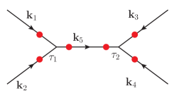
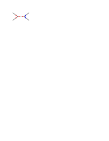
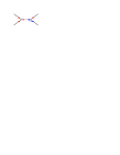
From Fig.1, it is straightforward to read the expressions for these integrals, we find

$$I_{a}\left(k_{1},k_{2},k_{3},k_{4},k_{5}\right)$$ (52)

$$\equiv -\frac{1}{2H^{2}}\Re\left[\int_{-\infty}^{\tau}d\tau_{1}\int_{-\infty}^{\tau_{1}}d\tau_{2}\frac{1}{\tau_{1}\tau_{2}}\partial_{1}G_{k_{1}}\left(\tau,\tau_{1}\right)\partial_{1}G_{k_{2}}\left(\tau,\tau_{1}\right)\partial_{2}G_{k_{3}}\left(\tau,\tau_{2}\right)\partial_{2}G_{k_{4}}\left(\tau,\tau_{2}\right)\partial_{12}G_{k_{5}}\left(\tau_{1},\tau_{2}\right)\right]$$

$$+\frac{1}{4H^{2}}\int_{-\infty}^{\tau}d\tau_{1}\int_{-\infty}^{\tau}d\tau_{2}\frac{1}{\tau_{1}\tau_{2}}\partial_{1}G_{k_{1}}\left(\tau_{1},\tau\right)\partial_{1}G_{k_{2}}\left(\tau_{1},\tau\right)\partial_{2}G_{k_{3}}\left(\tau,\tau_{2}\right)\partial_{2}G_{k_{4}}\left(\tau,\tau_{2}\right)\partial_{12}G_{k_{5}}\left(\tau_{1},\tau_{2}\right),$$

where and in what follows $\partial_{1,2}\equiv\frac{d}{d\tau_{1,2}}$, $\partial_{12}\equiv\frac{d^{2}}{d\tau_{1}d\tau_{2}}$ and in this appendix we denote $G_{k}(\tau_{1},\tau_{2})=u_{k}(\eta_{1})u^{\ast}_{k}(\eta_{2})$ with $u_{k}(\eta)=\frac{i\,H}{\sqrt{2k^{3}}}\left(1+ik\eta\right)e^{-ik\eta}$.

$$I_{b}^{\left(1\right)}\left(\bm{k}_{1},\bm{k}_{2},\bm{k}_{3},\bm{k}_{4},k_{5}\right)$$ (53)

$$\equiv -\frac{1}{2H^{2}}\left(\bm{k}_{1}\cdot\bm{k}_{2}\right)\left(\bm{k}_{3}\cdot\bm{k}_{4}\right)\Re\left[\int_{-\infty}^{\tau}d\tau_{1}\int_{-\infty}^{\tau_{1}}d\tau_{2}\frac{1}{\tau_{1}\tau_{2}}G_{k_{1}}\left(\tau,\tau_{1}\right)G_{k_{2}}\left(\tau,\tau_{1}\right)G_{k_{3}}\left(\tau,\tau_{2}\right)G_{k_{4}}\left(\tau,\tau_{2}\right)\partial_{12}G_{k_{5}}\left(\tau_{1},\tau_{2}\right)\right]$$

$$+\frac{1}{4H^{2}}\left(\bm{k}_{1}\cdot\bm{k}_{2}\right)\left(\bm{k}_{3}\cdot\bm{k}_{4}\right)\int_{-\infty}^{\tau}d\tau_{1}\int_{-\infty}^{\tau}d\tau_{2}\frac{1}{\tau_{1}\tau_{2}}G_{k_{1}}\left(\tau_{1},\tau\right)G_{k_{2}}\left(\tau_{1},\tau\right)G_{k_{3}}\left(\tau,\tau_{2}\right)G_{k_{4}}\left(\tau,\tau_{2}\right)\partial_{12}G_{k_{5}}\left(\tau_{1},\tau_{2}\right),$$

$$I_{b}^{\left(2\right)}\left(\bm{k}_{1},\bm{k}_{2},k_{3},\bm{k}_{4},\bm{k}_{5}\right)$$ (54)

$$\equiv -\frac{1}{2H^{2}}\left(\bm{k}_{1}\cdot\bm{k}_{2}\right)\left(\bm{k}_{5}\cdot\bm{k}_{4}\right)\Re\left[\int_{-\infty}^{\tau}d\tau_{1}\int_{-\infty}^{\tau_{1}}d\tau_{2}\frac{1}{\tau_{1}\tau_{2}}G_{k_{1}}\left(\tau,\tau_{1}\right)G_{k_{2}}\left(\tau,\tau_{1}\right)\partial_{2}G_{k_{3}}\left(\tau,\tau_{2}\right)G_{k_{4}}\left(\tau,\tau_{2}\right)\partial_{1}G_{k_{5}}\left(\tau_{1},\tau_{2}\right)\right]$$

$$+\frac{1}{4H^{2}}\left(\bm{k}_{1}\cdot\bm{k}_{2}\right)\left(\bm{k}_{5}\cdot\bm{k}_{4}\right)\int_{-\infty}^{\tau}d\tau_{1}\int_{-\infty}^{\tau}d\tau_{2}\frac{1}{\tau_{1}\tau_{2}}G_{k_{1}}\left(\tau_{1},\tau\right)G_{k_{2}}\left(\tau_{1},\tau\right)\partial_{2}G_{k_{3}}\left(\tau,\tau_{2}\right)G_{k_{4}}\left(\tau,\tau_{2}\right)\partial_{1}G_{k_{5}}\left(\tau_{1},\tau_{2}\right),$$

$$I_{b}^{\left(3\right)}\left(k_{1},\bm{k}_{2},k_{3},\bm{k}_{4},\bm{k}_{5}\right)$$ (55)

$$\equiv \frac{1}{2H^{2}}\left(\bm{k}_{5}\cdot\bm{k}_{2}\right)\left(\bm{k}_{5}\cdot\bm{k}_{4}\right)\Re\left[\int_{-\infty}^{\tau}d\tau_{1}\int_{-\infty}^{\tau_{1}}d\tau_{2}\frac{1}{\tau_{1}\tau_{2}}\partial_{1}G_{k_{1}}\left(\tau,\tau_{1}\right)G_{k_{2}}\left(\tau,\tau_{1}\right)\partial_{2}G_{k_{3}}\left(\tau,\tau_{2}\right)G_{k_{4}}\left(\tau,\tau_{2}\right)G_{k_{5}}\left(\tau_{1},\tau_{2}\right)\right]$$

$$-\frac{1}{4H^{2}}\left(\bm{k}_{5}\cdot\bm{k}_{2}\right)\left(\bm{k}_{5}\cdot\bm{k}_{4}\right)\int_{-\infty}^{\tau}d\tau_{1}\int_{-\infty}^{\tau}d\tau_{2}\frac{1}{\tau_{1}\tau_{2}}\partial_{1}G_{k_{1}}\left(\tau_{1},\tau\right)G_{k_{2}}\left(\tau_{1},\tau\right)\partial_{2}G_{k_{3}}\left(\tau,\tau_{2}\right)G_{k_{4}}\left(\tau,\tau_{2}\right)G_{k_{5}}\left(\tau_{1},\tau_{2}\right),$$

and

$$I_{c}^{\left(1\right)}\left(k_{1},k_{2},\bm{k}_{3},\bm{k}_{4},k_{5}\right)$$ (56)

$$\equiv \frac{1}{2H^{2}}\left(\bm{k}_{3}\cdot\bm{k}_{4}\right)\Re\int_{-\infty}^{\tau}d\tau_{1}\int_{-\infty}^{\tau_{1}}d\tau_{2}\frac{1}{\tau_{1}\tau_{2}}\partial_{1}G_{k_{1}}\left(\tau,\tau_{1}\right)\partial_{1}G_{k_{2}}\left(\tau,\tau_{1}\right)G_{k_{3}}\left(\tau,\tau_{2}\right)G_{k_{4}}\left(\tau,\tau_{2}\right)\partial_{12}G_{k_{5}}\left(\tau_{1},\tau_{2}\right)$$

$$-\frac{1}{4H^{2}}\left(\bm{k}_{3}\cdot\bm{k}_{4}\right)\int_{-\infty}^{\tau}d\tau_{1}\int_{-\infty}^{\tau}d\tau_{2}\frac{1}{\tau_{1}\tau_{2}}\partial_{1}G_{k_{1}}\left(\tau_{1},\tau\right)\partial_{1}G_{k_{2}}\left(\tau_{1},\tau\right)G_{k_{3}}\left(\tau,\tau_{2}\right)G_{k_{4}}\left(\tau,\tau_{2}\right)\partial_{12}G_{k_{5}}\left(\tau_{1},\tau_{2}\right),$$

$$I_{c}^{\left(2\right)}\left(k_{1},k_{2},k_{3},\bm{k}_{4},\bm{k}_{5}\right)$$ (57)

$$\equiv \frac{1}{2H^{2}}\left(\bm{k}_{5}\cdot\bm{k}_{4}\right)\Re\int_{-\infty}^{\tau}d\tau_{1}\int_{-\infty}^{\tau_{1}}d\tau_{2}\frac{1}{\tau_{1}\tau_{2}}\partial_{1}G_{k_{1}}\left(\tau,\tau_{1}\right)\partial_{1}G_{k_{2}}\left(\tau,\tau_{1}\right)\partial_{2}G_{k_{3}}\left(\tau,\tau_{2}\right)G_{k_{4}}\left(\tau,\tau_{2}\right)\partial_{1}G_{k_{5}}\left(\tau_{1},\tau_{2}\right)$$

$$-\frac{1}{4H^{2}}\left(\bm{k}_{5}\cdot\bm{k}_{4}\right)\int_{-\infty}^{\tau}d\tau_{1}\int_{-\infty}^{\tau}d\tau_{2}\frac{1}{\tau_{1}\tau_{2}}\partial_{1}G_{k_{1}}\left(\tau_{1},\tau\right)\partial_{1}G_{k_{2}}\left(\tau_{1},\tau\right)\partial_{2}G_{k_{3}}\left(\tau,\tau_{2}\right)G_{k_{4}}\left(\tau,\tau_{2}\right)\partial_{1}G_{k_{5}}\left(\tau_{1},\tau_{2}\right).$$

It is useful to introduce the “conjugate” contributions, defined as follows. Up to the second-order in perturbation theory, there are two interaction vertices and thus two temporal integrals with respect to $\tau_{1}$ and $\tau_{2}$ respectively. We call two contributions (diagrams) are conjugate to each other with exchanging $\tau_{1}\leftrightarrow\tau_{2}$ while keeping all the momenta relations. Having known the expression for a diagram, it is easy to write down the integral expression for its conjugate, e.g.

$$\tilde{I}_{a}\left(k_{1},k_{2},k_{3},k_{4},k_{12}\right)$$ (58)

$$\equiv -\frac{1}{2H^{2}}\Re\left[\int_{-\infty}^{\tau}d\tau_{1}\int_{-\infty}^{\tau_{1}}d\tau_{2}\frac{1}{\tau_{1}\tau_{2}}\partial_{2}G_{k_{1}}\left(\tau,\tau_{2}\right)\partial_{2}G_{k_{2}}\left(\tau,\tau_{2}\right)\partial_{1}G_{k_{3}}\left(\tau,\tau_{1}\right)\partial_{1}G_{k_{4}}\left(\tau,\tau_{1}\right)\partial_{12}G_{k_{5}}\left(\tau_{1},\tau_{2}\right)\right]$$

$$+\frac{1}{4H^{2}}\left[\int_{-\infty}^{\tau}d\tau_{1}\int_{-\infty}^{\tau}d\tau_{2}\frac{1}{\tau_{1}\tau_{2}}\partial_{1}G_{k_{1}}\left(\tau_{1},\tau\right)\partial_{1}G_{k_{2}}\left(\tau_{1},\tau\right)\partial_{2}G_{k_{3}}\left(\tau,\tau_{2}\right)\partial_{2}G_{k_{4}}\left(\tau,\tau_{2}\right)\partial_{12}G_{k_{5}}\left(\tau_{1},\tau_{2}\right)\right]^{\ast},$$

where $\ast$ denotes complex conjugate. It is analogous for the other conjugate integrals, which we do not write here for simplicity. Moreover, we introduce the combination of a contribution and its conjugate, e.g.

$$\mathcal{I}_{a}\left(k_{1},k_{2},k_{3},k_{4},k_{5}\right)\equiv[I_{a}+\tilde{I}_{a}]\left(k_{1},k_{2},k_{3},k_{4},k_{5}\right).$$ (59)

Before we evaluate the integrals, it is useful to make it clear about the smallest set of integrals we need. There are two cases. For left-right asymmetric diagrams, e.g. $I_{b}^{(2)}$ (or $\tilde{I}_{b}^{(2)}$), we always encounter the combination $\mathcal{I}_{b}^{(2)}\equiv I_{b}^{(2)}+\tilde{I}_{b}^{(2)}$ rather than $\tilde{I}_{b}^{(2)}$ itself. While for the left-right symmetric diagrams, e.g. $I_{a}$, $\tilde{I}_{a}$ is simply exchanging simultaneously $\bm{k}_{1}\leftrightarrow\bm{k}_{3}$ , $\bm{k}_{2}\leftrightarrow\bm{k}_{4}$. Thus, after the 6 permutations (which specify two momenta associated with $\tau_{1}$ and other two momenta associated with $\tau_{2}$) among the four extra momenta $\bm{k}_{1},\cdots,\bm{k}_{4}$, the final contribution to the correlation function from $I_{a}$ is equal to $\mathcal{I}_{a}/2$. Thus, what we really need is the following six basic integrals: $\mathcal{I}_{a}$, $\mathcal{I}_{b}^{(1)}$, $\mathcal{I}_{b}^{(2)}$, $\mathcal{I}_{b}^{(3)}$, $\mathcal{I}_{c}^{(1)}$ and $\mathcal{I}_{c}^{(2)}$.

Now we collect the final results for these integrals, in the limit of $\tau\rightarrow 0$. We find

$$\mathcal{I}_{a}\left(k_{1},k_{2},k_{3},k_{4},k_{5}\right)\equiv\frac{H^{8}k_{5}}{16K^{5}}\left(\prod_{i=1}^{4}\frac{1}{k_{i}}\right)\left[A\left(K_{12},K_{34},k_{5}\right)+\frac{K^{5}}{\left(K_{12}+k_{5}\right)^{3}\left(K_{34}+k_{5}\right)^{3}}\right]\,,$$ (60)

with

$$A\left(s_{1},s_{2},r\right)\equiv\frac{10s_{2}^{2}+\left(s_{1}+3r\right)\left(4s_{2}+K\right)+6r^{2}}{\left(s_{2}+r\right)^{3}}+\left(s_{1}\leftrightarrow s_{2}\right)\,,$$ (61)

where here and in what follows we denote $K_{ij}\equiv k_{i}+k_{j}$ and $K\equiv k_{1}+k_{2}+k_{3}+k_{4}$.

$$\mathcal{I}_{b}^{\left(1\right)}\left(\bm{k}_{1},\bm{k}_{2},\bm{k}_{3},\bm{k}_{4},k_{5}\right) =\left(\bm{k}_{1}\cdot\bm{k}_{2}\right)\left(\bm{k}_{3}\cdot\bm{k}_{4}\right)\frac{H^{8}k_{5}}{64K^{5}}\left(\prod_{i=1}^{4}\frac{1}{k_{i}^{3}}\right)$$ (62)

$$\times\left[\Gamma\left(K_{12},K_{34};k_{1}k_{2},k_{3}k_{4};J_{12}\right)+\left(12\leftrightarrow 34\right)+K^{5}F\left(K_{12},k_{5},k_{1}k_{2}\right)F\left(K_{34},k_{5},k_{3}k_{4}\right)\right].$$

with $J_{ij}\equiv K_{ij}-k_{5}$, and

$$\Gamma(s_{1},s_{2};q_{1},q_{2},t)\equiv \frac{1}{\left(K-t\right)^{3}}\left\{K^{6}+K^{5}\left(-2t+s_{1}+2s_{2}\right)\right.$$ (63)

$$+K^{4}\left[t\left(t-2s_{1}\right)+3\left(-t+s_{1}\right)s_{2}+2q_{1}+6q_{2}\right]$$

$$+K^{3}\left[t^{2}\left(s_{1}+s_{2}\right)+8s_{2}q_{1}+12s_{1}q_{2}-t\left(5s_{1}s_{2}+4q_{1}+6q_{2}\right)\right]$$

$$+K^{2}\left[2t\left(ts_{1}s_{2}+\left(t-7s_{2}\right)q_{1}\right)+2\left(t^{2}-8ts_{1}+20q_{1}\right)q_{2}\right]$$

$$\left.+6Kt\left[ts_{2}q_{1}+\left(ts_{1}-10q_{1}\right)q_{2}\right]+24t^{2}q_{1}q_{2}\right\}\,,$$

and

$$F\left(s,t,q\right)\equiv\frac{2s^{2}+2q+3st+t^{2}}{\left(s+t\right)^{3}}.$$ (64)

$$\mathcal{I}_{b}^{\left(2\right)}\left(\bm{k}_{1},\bm{k}_{2},k_{3},\bm{k}_{4},\bm{k}_{5}\right)$$ (65)

$$\equiv \left(\bm{k}_{1}\cdot\bm{k}_{2}\right)\left(\bm{k}_{4}\cdot\bm{k}_{5}\right)\left(\frac{k_{3}}{k_{5}}\right)^{2}\frac{H^{8}k_{5}}{64K^{5}}\left(\prod_{i=1}^{4}\frac{1}{k_{i}^{3}}\right)$$

$$\times\left[{\Gamma}\left(K_{12},K_{45};k_{1}k_{2},k_{4}k_{5};J_{12}\right)+{\Gamma}\left(\bar{K}_{45},K_{12};-k_{4}k_{5},k_{1}k_{2};J_{34}\right)+K^{5}F\left(K_{12},k_{5},k_{1}k_{2}\right)F\left(K_{45},k_{3},k_{4}k_{5}\right)\right]\,,$$

where $\bar{K}_{ij}\equiv k_{i}-k_{j}$.

$$\mathcal{I}_{b}^{\left(3\right)}\left(k_{1},\bm{k}_{2},k_{3},\bm{k}_{4},\bm{k}_{5}\right)$$ (66)

$$\equiv \left(-\bm{k}_{2}\cdot\bm{k}_{5}\right)\left(\bm{k}_{4}\cdot\bm{k}_{5}\right)\frac{k_{1}^{2}k_{3}^{2}}{k_{5}^{3}}\frac{H^{8}}{64K^{5}}\left(\prod_{i=1}^{4}\frac{1}{k_{i}^{3}}\right)$$

$$\times\left[{\Gamma}\left(\bar{K}_{25},K_{45};-k_{2}k_{5},k_{4}k_{5};J_{12}\right)+{\Gamma}\left(\bar{K}_{45},K_{25};-k_{4}k_{5},k_{2}k_{5};J_{34}\right)+K^{5}F\left(K_{25},k_{1},k_{2}k_{5}\right)F\left(K_{45},k_{3},k_{4}k_{5}\right)\right]\,.$$

And

$$\mathcal{I}_{c}^{\left(1\right)}\left(k_{1},k_{2},\bm{k}_{3},\bm{k}_{4},k_{5}\right)$$ (67)

$$\equiv \left(\bm{k}_{3}\cdot\bm{k}_{4}\right)\frac{H^{8}}{32K^{5}}\frac{k_{5}}{k_{1}k_{2}k_{3}^{3}k_{4}^{3}}\left[C\left(K_{34},k_{3}k_{4},J_{12}\right)+\bar{C}\left(K_{34},k_{3}k_{4},J_{34}\right)+\frac{K^{5}F\left(K_{34},k_{5},k_{3}k_{4}\right)}{\left(K_{12}+k_{5}\right)^{3}}\right]\,,$$

$$\mathcal{I}_{c}^{\left(2\right)}\left(k_{1},k_{2},k_{3},\bm{k}_{4},\bm{k}_{5}\right)$$ (68)

$$\equiv \left(\bm{k}_{5}\cdot\bm{k}_{4}\right)\frac{H^{8}}{32K^{5}}\frac{1}{k_{1}k_{2}k_{3}k_{4}^{3}k_{5}}\left[C\left(K_{45},k_{4}k_{5},J_{12}\right)+\bar{C}\left(\bar{K}_{45},-k_{4}k_{5},J_{34}\right)+\frac{K^{5}F\left(K_{45},k_{3},k_{4}k_{5}\right)}{\left(K_{12}+\tilde{k}_{5}\right)^{3}}\right]\,,$$

with

$$C\left(s,q,t\right) \equiv\frac{K\left(K-t\right)\left[-t\left(K+3s\right)+K\left(K+4s\right)\right]+2\left(10K^{2}-15Kt+6t^{2}\right)q}{\left(K-t\right)^{3}},$$ (69)

$$\bar{C}\left(s,q,t\right) \equiv\frac{K\left(3K^{2}\left(K+2s\right)+t^{2}\left(K+3s\right)-Kt\left(3K+8s\right)\right)+2\left(10K^{2}-15Kt+6t^{2}\right)q}{\left(K-t\right)^{3}}\,.$$

References

• [1] A. Guth, Phys. Rev. D 23 (1981) 347.
• [2] A. D. Miller et al., Astrophys. J.  524, L1 (1999) [arXiv:astro-ph/9906421].
• [3] P. de Bernardis et al. [Boomerang Collaboration], Nature 404, 955 (2000) [arXiv:astro-ph/0004404].
• [4] S. Hanany et al., Astrophys. J.  545, L5 (2000) [arXiv:astro-ph/0005123].
• [5] N. W. Halverson et al., Astrophys. J.  568, 38 (2002) [arXiv:astro-ph/0104489].
• [6] B. S. Mason et al., Astrophys. J.  591, 540 (2003) [arXiv:astro-ph/0205384].
• [7] E. Komatsu et al. [WMAP Collaboration], Astrophys. J. Suppl.  180, 330 (2009) [arXiv:0803.0547 [astro-ph]].
• [8] E. Komatsu et al., arXiv:1001.4538 [astro-ph.CO].
• [9] D. Larson et al., arXiv:1001.4635 [astro-ph.CO].
• [10] V. Mukhanov, and G. Chibisov, JETP 33, 549 (1981).
• [11] A. H. Guth, and S.-Y. Pi, Phys. Rev. Lett. 49, 1110 (1982).
• [12] S. W. Hawking, Phys. Lett. B115, 295 (1982).
• [13] A. A. Starobinsky, Phys. Lett. B117, 175 (1982).
• [14] J. M. Bardeen, P. J. Steinhardt, and M. S. Turner, Phys. Rev. D28, 679 (1983).
• [15] E. Komatsu et al., arXiv:0902.4759 [astro-ph.CO].
• [16] N. Bartolo, E. Komatsu, S. Matarrese and A. Riotto, Phys. Rept.  402, 103 (2004) [arXiv:astro-ph/0406398].
• [17] J. M. Maldacena, JHEP 0305, 013 (2003) [arXiv:astro-ph/0210603].
• [18] D. Seery and J. E. Lidsey, JCAP 0506, 003 (2005) [arXiv:astro-ph/0503692].
• [19] X. Chen, M. x. Huang, S. Kachru and G. Shiu, JCAP 0701, 002 (2007) [arXiv:hep-th/0605045].
• [20] X. Chen, M. x. Huang and G. Shiu, Phys. Rev.  D 74, 121301 (2006) [arXiv:hep-th/0610235].
• [21] C. Cheung, P. Creminelli, A. L. Fitzpatrick, J. Kaplan and L. Senatore, JHEP 0803, 014 (2008) [arXiv:0709.0293 [hep-th]].
• [22] X. Chen, R. Easther and E. A. Lim, JCAP 0706, 023 (2007) [arXiv:astro-ph/0611645].
• [23] X. Chen, R. Easther and E. A. Lim, JCAP 0804, 010 (2008) [arXiv:0801.3295 [astro-ph]].
• [24] D. Seery, J. E. Lidsey and M. S. Sloth, JCAP 0701, 027 (2007) [arXiv:astro-ph/0610210].
• [25] D. Seery and J. E. Lidsey, JCAP 0701, 008 (2007) [arXiv:astro-ph/0611034].
• [26] C. T. Byrnes, M. Sasaki and D. Wands, Phys. Rev.  D 74, 123519 (2006) [arXiv:astro-ph/0611075].
• [27] F. Arroja and K. Koyama, Phys. Rev.  D 77, 083517 (2008) [arXiv:0802.1167 [hep-th]].
• [28] D. Seery, M. S. Sloth and F. Vernizzi, JCAP 0903, 018 (2009) [arXiv:0811.3934 [astro-ph]].
• [29] X. Chen, B. Hu, M. x. Huang, G. Shiu and Y. Wang, JCAP 0908, 008 (2009) [arXiv:0905.3494 [astro-ph.CO]].
• [30] F. Arroja, S. Mizuno, K. Koyama and T. Tanaka, Phys. Rev.  D 80, 043527 (2009) [arXiv:0905.3641 [hep-th]].
• [31] C. Armendariz-Picon, T. Damour and V. F. Mukhanov, Phys. Lett.  B 458, 209 (1999) [arXiv:hep-th/9904075].
• [32] J. Garriga and V. F. Mukhanov, Phys. Lett.  B 458, 219 (1999) [arXiv:hep-th/9904176].
• [33] N. Bartolo, M. Fasiello, S. Matarrese and A. Riotto, JCAP 1008 (2010) 008 [arXiv:1004.0893 [astro-ph.CO]].
• [34] N. Bartolo, M. Fasiello, S. Matarrese and A. Riotto, arXiv:1006.5411 [astro-ph.CO].
• [35] N. Bartolo, S. Matarrese and A. Riotto, Phys. Rev.  D 65, 103505 (2002) [arXiv:hep-ph/0112261].
• [36] D. Seery and J. E. Lidsey, JCAP 0509, 011 (2005) [arXiv:astro-ph/0506056].
• [37] D. Langlois, S. Renaux-Petel, D. A. Steer and T. Tanaka, Phys. Rev.  D 78, 063523 (2008) [arXiv:0806.0336 [hep-th]].
• [38] D. Langlois, S. Renaux-Petel, D. A. Steer and T. Tanaka, Phys. Rev. Lett.  101, 061301 (2008) [arXiv:0804.3139 [hep-th]].
• [39] D. Langlois, S. Renaux-Petel and D. A. Steer, JCAP 0904, 021 (2009) [arXiv:0902.2941 [hep-th]].
• [40] S. Renaux-Petel, JCAP 0910 (2009) 012 [arXiv:0907.2476 [hep-th]].
• [41] X. Gao, JCAP 0806, 029 (2008) [arXiv:0804.1055 [astro-ph]].
• [42] X. Gao and B. Hu, JCAP 0908 (2009) 012 [arXiv:0903.1920 [astro-ph.CO]].
• [43] F. Arroja, S. Mizuno and K. Koyama, JCAP 0808, 015 (2008) [arXiv:0806.0619 [astro-ph]].
• [44] E. Kawakami, M. Kawasaki, K. Nakayama and F. Takahashi, JCAP 0909, 002 (2009) [arXiv:0905.1552 [astro-ph.CO]].
• [45] S. Mizuno, F. Arroja, K. Koyama and T. Tanaka, Phys. Rev.  D 80, 023530 (2009) [arXiv:0905.4557 [hep-th]].
• [46] S. Mizuno, F. Arroja and K. Koyama, Phys. Rev.  D 80 (2009) 083517 [arXiv:0907.2439 [hep-th]].
• [47] J. L. Lehners and S. Renaux-Petel, Phys. Rev.  D 80, 063503 (2009) [arXiv:0906.0530 [hep-th]].
• [48] F. Bernardeau and J. P. Uzan, Phys. Rev.  D 66, 103506 (2002) [arXiv:hep-ph/0207295].
• [49] D. Wands, N. Bartolo, S. Matarrese and A. Riotto, Phys. Rev.  D 66, 043520 (2002) [arXiv:astro-ph/0205253].
• [50] C. T. Byrnes, K. Y. Choi and L. M. H. Hall, JCAP 0810, 008 (2008) [arXiv:0807.1101 [astro-ph]].
• [51] C. T. Byrnes, K. Y. Choi and L. M. H. Hall, JCAP 0902, 017 (2009) [arXiv:0812.0807 [astro-ph]].
• [52] D. Battefeld and T. Battefeld, JCAP 0911 (2009) 010 [arXiv:0908.4269 [hep-th]].
• [53] D. Langlois, F. Vernizzi and D. Wands, JCAP 0812, 004 (2008) [arXiv:0809.4646 [astro-ph]].
• [54] M. Kawasaki, K. Nakayama, T. Sekiguchi, T. Suyama and F. Takahashi, JCAP 0811, 019 (2008) [arXiv:0808.0009 [astro-ph]].
• [55] D. Langlois and S. Renaux-Petel, JCAP 0804, 017 (2008) [arXiv:0801.1085 [hep-th]].
• [56] G. I. Rigopoulos, E. P. S. Shellard and B. J. W. van Tent, Phys. Rev.  D 73, 083521 (2006) [arXiv:astro-ph/0504508].
• [57] X. d. Ji and T. Wang, Phys. Rev.  D 79, 103525 (2009) [arXiv:0903.0379 [hep-th]].
• [58] S. Pi and T. Wang, Phys. Rev.  D 80, 043503 (2009) [arXiv:0905.3470 [astro-ph.CO]].
• [59] D. A. Easson, R. Gregory, D. F. Mota, G. Tasinato and I. Zavala, JCAP 0802, 010 (2008) [arXiv:0709.2666 [hep-th]].
• [60] M. x. Huang, G. Shiu and B. Underwood, Phys. Rev.  D 77, 023511 (2008) [arXiv:0709.3299 [hep-th]].
• [61] Y. F. Cai and W. Xue, Phys. Lett.  B 680, 395 (2009) [arXiv:0809.4134 [hep-th]].
• [62] Y. F. Cai and H. Y. Xia, Phys. Lett.  B 677, 226 (2009) [arXiv:0904.0062 [hep-th]].
• [63] X. Gao, JCAP 1002 (2010) 019 [arXiv:0908.4035 [hep-th]].
• [64] T. Wang, arXiv:1008.3198 [astro-ph.CO].
• [65] A. S. Sakharov and M. Y. Khlopov, Phys. Atom. Nucl.  56 (1993) 412 [Yad. Fiz.  56N3 (1993) 220].
• [66] D. I. Kaiser and A. T. Todhunter, Phys. Rev.  D 81 (2010) 124037 [arXiv:1004.3805 [astro-ph.CO]].
• [67] C. M. Peterson and M. Tegmark, arXiv:1005.4056 [astro-ph.CO].
• [68] M. Sasaki, J. Valiviita and D. Wands, Phys. Rev.  D 74, 103003 (2006) [arXiv:astro-ph/0607627].
• [69] K. A. Malik and D. H. Lyth, JCAP 0609, 008 (2006) [arXiv:astro-ph/0604387].
• [70] Q. G. Huang and Y. Wang, JCAP 0809, 025 (2008) [arXiv:0808.1168 [hep-th]].
• [71] Q. G. Huang, JCAP 0809, 017 (2008) [arXiv:0807.1567 [hep-th]].
• [72] Q. G. Huang, Phys. Lett.  B 669, 260 (2008) [arXiv:0801.0467 [hep-th]].
• [73] S. Li, Y. F. Cai and Y. S. Piao, Phys. Lett.  B 671, 423 (2009) [arXiv:0806.2363 [hep-ph]].
• [74] K. Ichikawa, T. Suyama, T. Takahashi and M. Yamaguchi, Phys. Rev.  D 78, 023513 (2008) [arXiv:0802.4138 [astro-ph]].
• [75] T. Kobayashi and S. Mukohyama, JCAP 0907, 032 (2009) [arXiv:0905.2835 [hep-th]].
• [76] M. Li, C. Lin, T. Wang and Y. Wang, Phys. Rev.  D 79, 063526 (2009) [arXiv:0805.1299 [astro-ph]].
• [77] L. Alabidi, JCAP 0610, 015 (2006) [arXiv:astro-ph/0604611].
• [78] M. Sasaki, Prog. Theor. Phys.  120, 159 (2008) [arXiv:0805.0974 [astro-ph]].
• [79] A. Naruko and M. Sasaki, Prog. Theor. Phys.  121, 193 (2009) [arXiv:0807.0180 [astro-ph]].
• [80] Q. G. Huang, JCAP 0905, 005 (2009) [arXiv:0903.1542 [hep-th]].
• [81] Q. G. Huang, JCAP 0906, 035 (2009) [arXiv:0904.2649 [hep-th]].
• [82] J. O. Gong, C. Lin and Y. Wang, JCAP 1003, 004 (2010) [arXiv:0912.2796 [astro-ph.CO]].
• [83] C. Lin and Y. Wang, JCAP 1007 (2010) 011 [arXiv:1004.0461 [astro-ph.CO]].
• [84] J. Zhang, Y. F. Cai and Y. S. Piao, JCAP 1005 (2010) 001 [arXiv:0912.0791 [hep-th]].
• [85] Y. F. Cai and Y. Wang, arXiv:1005.0127 [hep-th].
• [86] D. M. Regan and E. P. S. Shellard, arXiv:0911.2491 [astro-ph.CO].
• [87] M. Hindmarsh, C. Ringeval and T. Suyama, Phys. Rev.  D 80 (2009) 083501 [arXiv:0908.0432 [astro-ph.CO]].
• [88] M. Hindmarsh, C. Ringeval and T. Suyama, Phys. Rev.  D 81 (2010) 063505 [arXiv:0911.1241 [astro-ph.CO]].
• [89] J. Kumar, L. Leblond and A. Rajaraman, JCAP 1004 (2010) 024 [arXiv:0909.2040 [astro-ph.CO]].
• [90] H. R. S. Cogollo, Y. Rodriguez and C. A. Valenzuela-Toledo, JCAP 0808 (2008) 029 [arXiv:0806.1546 [astro-ph]].
• [91] Y. Rodriguez and C. A. Valenzuela-Toledo, Phys. Rev.  D 81 (2010) 023531 [arXiv:0811.4092 [astro-ph]].
• [92] P. D. Meerburg, J. P. van der Schaar and P. S. Corasaniti, JCAP 0905 (2009) 018 [arXiv:0901.4044 [hep-th]].
• [93] P. D. Meerburg, J. P. van der Schaar and M. G. Jackson, JCAP 1002 (2010) 001 [arXiv:0910.4986 [hep-th]].
• [94] Q. G. Huang, JCAP 1007 (2010) 025 [arXiv:1004.0808 [astro-ph.CO]].
• [95] K. Izumi and S. Mukohyama, JCAP 1006 (2010) 016 [arXiv:1004.1776 [hep-th]].
• [96] X. Chen and Y. Wang, Phys. Rev.  D 81 (2010) 063511 [arXiv:0909.0496 [astro-ph.CO]].
• [97] X. Chen and Y. Wang, JCAP 1004, 027 (2010) [arXiv:0911.3380 [hep-th]].
• [98] C. A. Valenzuela-Toledo and Y. Rodriguez, Phys. Lett.  B 685 (2010) 120 [arXiv:0910.4208 [astro-ph.CO]].
• [99] N. Bartolo, E. Dimastrogiovanni, S. Matarrese and A. Riotto, JCAP 0911 (2009) 028 [arXiv:0909.5621 [astro-ph.CO]].
• [100] N. Bartolo, E. Dimastrogiovanni, S. Matarrese and A. Riotto, JCAP 0910 (2009) 015 [arXiv:0906.4944 [astro-ph.CO]].
• [101] C. A. Valenzuela-Toledo, Y. Rodriguez and D. H. Lyth, Phys. Rev.  D 80 (2009) 103519 [arXiv:0909.4064 [astro-ph.CO]].
• [102] E. Dimastrogiovanni, N. Bartolo, S. Matarrese and A. Riotto, arXiv:1001.4049 [astro-ph.CO].
• [103] M. Karciauskas, K. Dimopoulos and D. H. Lyth, Phys. Rev.  D 80 (2009) 023509 [arXiv:0812.0264 [astro-ph]].
• [104] X. Gao, M. Li and C. Lin, JCAP 0911, 007 (2009) [arXiv:0906.1345 [astro-ph.CO]].
• [105] X. Chen, B. Hu, M. x. Huang, G. Shiu and Y. Wang, JCAP 0908, 008 (2009) [arXiv:0905.3494 [astro-ph.CO]].
• [106] V. F. Mukhanov, H. A. Feldman and R. H. Brandenberger, Phys. Rept.  215, 203 (1992).
• [107] R. H. Brandenberger, Lect. Notes Phys.  646, 127 (2004) [arXiv:hep-th/0306071].
• [108] S. Weinberg, Phys. Rev.  D 72, 043514 (2005) [arXiv:hep-th/0506236].
• [109] P. Creminelli and M. Zaldarriaga, JCAP 0410 (2004) 006 [arXiv:astro-ph/0407059].
• [110] J. Ganc and E. Komatsu, arXiv:1006.5457 [astro-ph.CO].
• [111] S. Renaux-Petel, arXiv:1008.0260 [astro-ph.CO].
• [112] J. R. Fergusson, M. Liguori and E. P. S. Shellard, Phys. Rev.  D 82 (2010) 023502 [arXiv:0912.5516 [astro-ph.CO]].
• [113] D. Munshi, A. Heavens, A. Cooray, J. Smidt, P. Coles and P. Serra, arXiv:0910.3693 [astro-ph.CO].
• [114] S. Mizuno and K. Koyama, arXiv:1007.1462 [hep-th].
• [115] D. M. Regan and E. P. S. Shellard, Phys. Rev.  D 82 (2010) 023520 [arXiv:1004.2915 [astro-ph.CO]].
• [116] T. Battefeld and R. Easther, JCAP 0703 (2007) 020 [arXiv:astro-ph/0610296].
• [117] D. Battefeld and T. Battefeld, JCAP 0705 (2007) 012 [arXiv:hep-th/0703012].
• [118] J. Smidt, A. Amblard, C. T. Byrnes, A. Cooray, A. Heavens and D. Munshi, Phys. Rev.  D 81 (2010) 123007 [arXiv:1004.1409 [astro-ph.CO]].