Limit theorems for the discrete-time quantum walk
on a graph with joined half lines

Abstract. We consider a discrete-time quantum walk $W_{t,\kappa}$ at time $t$ on a graph with joined half lines $\mathbb{J}_{\kappa}$, which is composed of $\kappa$ half lines with the same origin. Our analysis is based on a reduction of the walk on a half line. The idea plays an important role to analyze the walks on some class of graphs with symmetric initial states. In this paper, we introduce a quantum walk with an enlarged basis and show that $W_{t,\kappa}$ can be reduced to the walk on a half line even if the initial state is asymmetric. For $W_{t,\kappa}$, we obtain two types of limit theorems. The first one is an asymptotic behavior of $W_{t,\kappa}$ which corresponds to localization. For some conditions, we find that the asymptotic behavior oscillates. The second one is the weak convergence theorem for $W_{t,\kappa}$. On each half line, $W_{t,\kappa}$ converges to a density function like the case of the one-dimensional lattice with a scaling order of $t$. The results contain the cases of quantum walks starting from the general initial state on a half line with the general coin and homogeneous trees with the Grover coin.

1 Introduction

Random walks have a very important role in various fields, such as physical systems, mathematical modeling and computer algorithms. In 1990s, quantum walks arise as a quantum counterpart of random walks [1, 2, 3]. They are defined by unitary evolutions of probability amplitudes, whereas random walks are obtained by evolutions of probabilities by transition matrices. Discrete-time quantum walks are introduced by Refs. [1, 2]. In recent years, quantum walks have been well developed in fields of quantum algorithms, for example [4, 5, 6]. On the other hand, studies of the walks from the mathematical point of view also arise. Especially, as a limiting behaver, localization appears in quantum cases [7, 8, 9, 10, 11, 12]. Furthermore the quantum walk has a quadratically faster scaling order than the random walk in the weak convergence [13, 14, 15, 16, 17]. Cantero et al. introduced an analysis using the CMV matrix [11, 12]. This method is very useful to consider localization. To analyze the quantum walk, we use the generating function. By using the generating function, we can compute not only localization but also the weak convergence of the walk. A reduction technique [20, 21, 22], which reduces the walk to a one-dimensional quantum walk, is very important to apply a path counting method [13, 14, 23] which gives an explicit expression for the generating function. To treat the quantum walk with asymmetric initial states, we introduce a quantum walk with enlarged bases.

Our main results are two limit theorems for the quantum walk ${W_{t,\kappa}}$ on a graph with joined half lines with arbitrary initial state starting from the origin. In case of $\kappa=1$, $W_{t,1}$ corresponds to a quantum walk on a half line with the general coin. Furthermore, by considering the reduction of the walks, the two limit theorems can be adopted to quantum walks on homogeneous trees and semi-homogeneous trees with the Grover coin operator. One of two our main results is the explicit expression for the limit probability of ${W_{t,\kappa}}$. It is corresponding to localization which is defined that there exists a vertex of the graph $x$ such that $\limsup_{t\to\infty}P({W_{t,\kappa}}=x)>0$. We find that, for some conditions, the asymptotic behavior oscillates. Same as other results on quantum walks [7, 8, 9], localization has an exponential decay for position $x$ on each half line. Another main result is the weak convergence of ${W_{t,\kappa}}$. On each half line, ${W_{t,\kappa}}$ has a scaling order $t$. Moreover the limit measure has a typical density function which appears on other quantum walks [8, 13, 14, 15, 16, 17].

For related works, Chisaki et al. [8] obtained the same type of limit theorems for a quantum walk on homogeneous trees with two special initial states. This result induces limit theorems for a quantum walk on a half line with a special coin operator. Konno and Segawa [18] showed localization of quantum walks on a half line by using the spectral analysis of the corresponding CMV matrices.

The remainder of the present paper is organized as follows. In Section 2, we give definitions of discrete-time quantum walks treated in this paper. Section 3 presents our results. Section 4 gives proofs of our main theorems. In Subsection 4.1, we introduce a quantum walk with an enlarged basis and reduce $W_{t,\kappa}$ to the walk on a half line. Subsection 4.2 presents a proof of Theorem 1 based on the generating function. Subsection 4.3 is devoted to a proof of Theorem 2 using the Fourier transform of the generating function. In Appendix, we compute the generating function.

2 Discrete-time quantum walks

This section gives the definition of the quantum walk on undirected connected graph $\mathbb{G}$. Let $V(\mathbb{G})$ be a set of all vertices in $\mathbb{G}$ and $E(\mathbb{G})$ be a set of all edges in $\mathbb{G}$. Here we define $E_{x}(\mathbb{G})\subset E(\mathbb{G})$ as a set of all edges which connect the vertex $x\in V(\mathbb{G})$. Now we take a Hilbert space spanned by an orthonormal basis $\{|{x}\rangle;\ x\in V(\mathbb{G})\}$ as a position space $\mathscr{H}_{p}$ and a Hilbert space generated by an orthonormal basis $\{|{l}\rangle;\ l\in E_{x}(\mathbb{G})\}$ for $x\in V(\mathbb{G})$ as a local coin space $\mathscr{H}_{c_{x}}$. A discrete-time quantum walk on $\mathbb{G}$ is defined on a Hilbert space $\mathscr{H}$ spanned by an orthonormal basis $\{|{x,l}\rangle;\ x\in V(\mathbb{G}),\ l\in E_{x}(\mathbb{G})\}$. Note that if we take $\mathbb{G}$ as a regular graph, $\mathscr{H}$ can be written as $\mathscr{H}=\mathscr{H}_{p}\otimes\mathscr{H}_{c_{x}}$ for any $x\in V(G)$. On the space $\mathscr{H}$, the evolution operator $U$ is given by $U=SF$, where $S:\mathscr{H}\to\mathscr{H}$ is a shift operator and $F:\mathscr{H}\to\mathscr{H}$ is a coin operator. Here we define $F=\sum_{x\in V(\mathbb{G})}|{x}\rangle\langle{x}|\otimes C_{x}$ as a coin operator and $C_{x}:\mathscr{H}_{c_{x}}\to\mathscr{H}_{c_{x}}$ for $x\in V(\mathbb{G})$ as a local coin operator. If the graph is regular and the local coin operator is all the same, we can rewrite the coin operator as $F=I_{p}\otimes C$, where $I_{p}$ is the identity operator on $\mathscr{H}_{p}$. As typical local coin operators, the Hadamard operator $H$ and the Grover operator $G_{d}$ are often used, where $H$ and $G_{d}$ $(d\geq 2)$ are defined by

$$H= \frac{1}{\sqrt{2}}\left[\begin{array}[]{cc}1&1\\ 1&-1\\ \end{array}\right],$$

$$G_{d}= \left[\begin{array}[]{cccc}a_{d}&b_{d}&\cdots&b_{d}\\ b_{d}&a_{d}&\cdots&b_{d}\\ \vdots&\vdots&\ddots&\vdots\\ b_{d}&b_{d}&\cdots&a_{d}\\ \end{array}\right]=\left[\begin{array}[]{cccc}\frac{2}{d}-1&\frac{2}{d}&\cdots&\frac{2}{d}\\ \frac{2}{d}&\frac{2}{d}-1&\cdots&\frac{2}{d}\\ \vdots&\vdots&\ddots&\vdots\\ \frac{2}{d}&\frac{2}{d}&\cdots&\frac{2}{d}-1\\ \end{array}\right].$$

In this paper we define $a_{1}=1$, $b_{1}=2$ and $G_{1}=1$. From the construction, the state at time $t$ and position $x$ is described as

$$\Psi_{t}(x) = \sum_{l\in E_{x}(\mathbb{G})}\alpha_{t}(x,l)|{x,l}\rangle,$$ (2.1)

where $\alpha_{t}(x,l)\in\mathbb{C}$ is the amplitude of the base $|{x,l}\rangle$ at time $t$ and $\mathbb{C}$ is the set of all complex numbers. The probability of the state is given by a square norm of $\Psi_{t}(x)$, i.e., $\|\Psi_{t}(x)\|^{2}=\sum_{l\in E_{x}(\mathbb{G})}|\alpha_{t}(x,l)|^{2}$. We only consider the initial state starting from the origin “$o$” with the state $\Psi_{0}(o)$ such that $\|\Psi_{0}(o)\|=1$.

2.1 Quantum walk on a graph with joined half lines

This subsection gives the definition of a graph with joined half lines ${\mathbb{J}_{\kappa}}$ and the quantum walk ${W_{t,\kappa}}$ on ${\mathbb{J}_{\kappa}}$. Let ${\mathbb{K}_{\kappa}}=\{0,1,\ldots,\kappa-1\}$ and $\mathbb{Z}_{r}=\{{h_{r}}(1),{h_{r}}(2),\ldots\}$ for $r\in{\mathbb{K}_{\kappa}}$, we define $V(\mathbb{J}_{\kappa})=\{0\}\cup\{\cup_{j\in\mathbb{K}_{\kappa}}\mathbb{Z}_{j}\}$. A vertex $h_{i}(x)$ connects $h_{j}(y)$ if and only if $|x-y|=1$ with $i=j$, and the origin $0$ connects $h_{r}(1)$ for any $r$ (see Fig. 1 (a) for example).

The quantum walk on ${\mathbb{J}_{\kappa}}$ is defined on $\mathscr{H}^{({\mathbb{J}_{\kappa}})}$ which is a Hilbert space spanned by an orthonormal basis $\{|{0,l}\rangle;\ l\in\{\epsilon_{0},\epsilon_{1},\ldots,\epsilon_{\kappa-1}\}\}\cup\{|{x,l}\rangle;\ x\in V({\mathbb{J}_{\kappa}})\setminus\{0\},\ l\in\{Up,Down\}\}$. Throughout this paper, we put the base $|{\epsilon_{r}}\rangle$ as ${}^{T}[\overbrace{0\cdots 0}^{r}1\overbrace{0\cdots 0}^{\kappa-r-1}],$ where $T$ is the transposed operator. We define a local coin operator $C$ as

$$C=\begin{bmatrix}a&b\\ c&d\end{bmatrix}\in U(2)\mathrm{\;with}\;abcd\neq 0,$$ (2.2)

where $U(d)$ is the set of $d\times d$ unitary matrices. The coin operator $F_{J}$ is given by

$$F_{J}=|{0}\rangle\langle{0}|\otimes G_{\kappa}+\sum_{x\in V({\mathbb{J}_{\kappa}})\setminus\{0\}}|{x}\rangle\langle{x}|\otimes C,$$ (2.3)

where $G_{\kappa}$ is the Grover operator. The shift operator $S_{J}$ is given by

$$S_{J}|{0,l}\rangle = |{{h_{r}}(1),Down}\rangle\ ,\ l=\epsilon_{r},$$

$$S_{J}|{{h_{r}}(1),l}\rangle = \left\{\begin{array}[]{ll}|{0,\epsilon_{r}}\rangle,&l=Up,\\ |{{h_{r}}(2),Down}\rangle,&l=Down,\\ \end{array}\right.$$

$$S_{J}|{{h_{r}}(x),l}\rangle = \left\{\begin{array}[]{ll}|{{h_{r}}(x-1),Up}\rangle,&l=Up,\\ |{{h_{r}}(x+1),Down}\rangle,&l=Down,\\ \end{array}\right.\ x\geq 2.$$

Then the evolution operator of the walk $U_{J}$ is obtained by $U_{J}=S_{J}F_{J}$. An expression of $W_{t,3}$ using weights is shown in Fig. 1 (a), where

$$P_{1}^{\epsilon_{1}}=\left[\begin{array}[]{cc}a&b\\ 0&0\\ 0&0\\ \end{array}\right], Q_{0}^{\epsilon_{1}}=\left[\begin{array}[]{ccc}0&0&0\\ -\frac{1}{3}&\frac{2}{3}&\frac{2}{3}\\ \end{array}\right],$$

$$P_{1}^{\epsilon_{2}}=\left[\begin{array}[]{cc}0&0\\ a&b\\ 0&0\\ \end{array}\right], Q_{0}^{\epsilon_{2}}=\left[\begin{array}[]{ccc}0&0&0\\ \frac{2}{3}&-\frac{1}{3}&\frac{2}{3}\\ \end{array}\right],$$

$$P_{1}^{\epsilon_{3}}=\left[\begin{array}[]{cc}0&0\\ 0&0\\ a&b\\ \end{array}\right], Q_{0}^{\epsilon_{3}}=\left[\begin{array}[]{ccc}0&0&0\\ \frac{2}{3}&\frac{2}{3}&-\frac{1}{3}\\ \end{array}\right],$$

$$P=\left[\begin{array}[]{cc}a&b\\ 0&0\\ \end{array}\right], Q=\left[\begin{array}[]{cc}0&0\\ c&d\\ \end{array}\right].$$

Note that $W_{t,1}$ is a quantum walk on a half line with a reflecting wall.

(a)	(b)

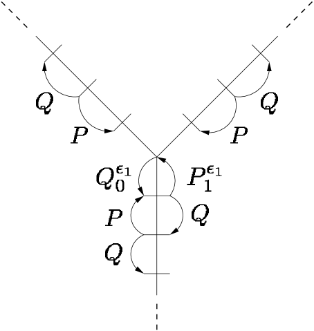
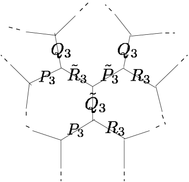
Figure 1: (a) Quantum walk on $\mathbb{J}_{3}$, (b) Quantum walk on $\mathbb{T}_{3}$

2.2 Quantum walk on homogeneous trees

We define a homogeneous tree $\mathbb{T}_{\kappa}$ and a quantum walk ${V_{t,\kappa}}$ on $\mathbb{T}_{\kappa}$. Fix $\kappa\geq 2$, let $\Sigma=\{{\sigma_{0}},{\sigma_{1}},\ldots,{\sigma_{\kappa-1}}\}$ be the set of generators subjected to the relation ${\sigma_{j}}^{2}=e$ for $j\in{\mathbb{K}_{\kappa}}$, where the empty word $e$ is the unit of this group. Then we put $V(\mathbb{T}_{\kappa})=\{e\}\cup\{{\sigma_{i_{n}}}\ldots{\sigma_{i_{2}}}{\sigma_{i_{1}}}:n\geq 1,\ {\sigma_{i_{j}}}\in\Sigma,\ i_{j+1}\neq i_{j}\ \mathrm{for}\ j=1,2,\ldots,n-1\}$. Here vertices $g$ and $h$ are connected if and only if $gh^{-1}\in\Sigma$. On this graph, $\mathscr{H}_{p}^{(\mathbb{T}_{\kappa})}$ is generated by an orthonormal basis $\{|{g}\rangle;\ g\in V(\mathbb{T}_{\kappa})\}$ and $\mathscr{H}_{c}^{(\mathbb{T}_{\kappa})}$ is associated with an orthonormal basis $\{|{{\sigma_{j}}}\rangle;\ {\sigma_{j}}\in\Sigma\}$. We choose $G_{\kappa}$ as the local coin operator, then the coin operator $F_{T}$ and the shift operator $S_{T}$ are defined as follows: for $\sigma\in\Sigma$

$$F_{T}=|{e}\rangle\langle{e}|\otimes\tilde{c}G_{\kappa}+\sum_{g\in V(\mathbb{T}_{\kappa})\setminus\{e\}}|{g}\rangle\langle{g}|\otimes G_{\kappa},$$

$$S_{T}|{g,\sigma}\rangle=|{\sigma g,\sigma}\rangle,$$

where we put $|{{\sigma_{r}}}\rangle$ as ${}^{T}[\overbrace{0\cdots 0}^{r}1\overbrace{0\cdots 0}^{\kappa-r-1}]$ and $\tilde{c}\in\mathbb{C}$ with $|\tilde{c}|=1$. The phase $\tilde{c}$ works as a defect on the origin, which is an extension of our model in [8]. An expression of $V_{t,3}$ using weights is shown in Fig. 1 (b), where

$$P_{3}=\left[\begin{array}[]{ccc}-\frac{1}{3}&\frac{2}{3}&\frac{2}{3}\\ 0&0&0\\ 0&0&0\\ \end{array}\right],\ Q_{3}=\left[\begin{array}[]{ccc}0&0&0\\ \frac{2}{3}&-\frac{1}{3}&\frac{2}{3}\\ 0&0&0\\ \end{array}\right],\ R_{3}=\left[\begin{array}[]{ccc}0&0&0\\ 0&0&0\\ \frac{2}{3}&\frac{2}{3}&-\frac{1}{3}\\ \end{array}\right],$$

and $\tilde{P}_{3}=\tilde{c}P_{3}$, $\tilde{Q}_{3}=\tilde{c}Q_{3}$, $\tilde{R}_{3}=\tilde{c}R_{3}$.

In the case of the one point initial state on the origin, $V_{t,\kappa}$ can be reduced to the equivalent walk on $\mathbb{J}_{\kappa}$ even if the initial state is not symmetric. To explain it, we define subgraph $\mathbb{T}_{\kappa}^{(r)}\in\mathbb{T}_{\kappa}$ as $V(\mathbb{T}_{\kappa}^{(r)})=\{\sigma_{i_{n}}\cdots\sigma_{i_{2}}\sigma_{i_{1}}:n\geq 1,\;\sigma_{i_{j}}\in\Sigma,\;\sigma_{i_{1}}=\sigma_{r},\;i_{j+1}\neq i_{j}\;\mathrm{for}\;j=1,2,\dots,n-1\}$. They are subtrees whose roots are the children of the root of $\mathbb{T}_{\kappa}$. Now we consider the following new basis, for $x\geq 1$,

$$|x,Up\rangle_{\sigma_{r}} =\frac{1}{\sqrt{(\kappa-1)^{x-1}}}\sum_{\scriptsize{\begin{matrix}g\in V(\mathbb{T}_{\kappa}^{(r)})\\ |g|=x\end{matrix}}}\sum_{\sigma_{j}:|\sigma_{j}g|=x-1}|g,\sigma_{j}\rangle,$$

$$|x,Down\rangle_{\sigma_{r}} =\frac{1}{\sqrt{(\kappa-1)^{x}}}\sum_{\scriptsize{\begin{matrix}g\in V(\mathbb{T}_{\kappa}^{(r)})\\ |g|=x\end{matrix}}}\sum_{\sigma_{j}:|\sigma_{j}g|=x+1}|g,\sigma_{j}\rangle.$$

The new space ${\mathscr{H}^{(\mathbb{T}_{\kappa})}}^{\prime}$ spanned by a basis $\{|e,l\rangle:l\in\Sigma\}\cup\{|x,l\rangle_{\sigma_{r}}:r\in\mathbb{K}_{\kappa},x\in\mathbb{Z}_{+},l\in\{Up,Down\}\}$ is isomorphic to ${\mathscr{H}^{(\mathbb{J}_{\kappa})}}$ under the following one-to-one correspondence

$$|x,l\rangle_{\sigma_{r}} \leftrightarrow|h_{r}(x),l\rangle\;\mathrm{for}\;l\in\{Up,Down\},\;x\geq 1,$$

$$|e,\sigma_{r}\rangle \leftrightarrow|0,\epsilon_{r}\rangle,$$ (2.11)

where $\mathbb{Z}_{+}=\{1,2,\dots\}$. Then the direct computation gives the following lemma.

Lemma 1 (Homogeneous tree)

The subspace of ${\mathscr{H}^{(\mathbb{T}_{\kappa})}}^{\prime}$ is invariant under the action of the time evolution of $V_{t,\kappa}$. In particular, when we take the bijection from ${\mathscr{H}^{(\mathbb{T}_{\kappa})}}^{\prime}$ to $\mathscr{H}^{(\mathbb{J}_{\kappa})}$ given by Eq. (2.11), the walk is equivalent to $W_{t,\kappa}$ with the following coin operator

$$F_{J}^{(\mathbb{T}_{\kappa})}=|{0}\rangle\langle{0}|\otimes\tilde{c}G_{\kappa}+\sum_{x\in V({\mathbb{J}_{\kappa}})\setminus\{0\}}|{x}\rangle\langle{x}|\otimes\left[\begin{array}[]{cc}a_{\kappa}&\sqrt{\kappa-1}b_{\kappa}\\ \sqrt{\kappa-1}b_{\kappa}&-a_{\kappa}\\ \end{array}\right].$$

When we consider $\tilde{c}^{-1}F_{J}^{(\mathbb{T}_{\kappa})}$, the above equation becomes a special case of Eq. (2.3), since $|\tilde{c}|=1$.

Similar to ${V_{t,\kappa}}$, we can define a quantum walk $V_{t,\kappa^{\prime},\kappa}$ on a semi-homogeneous tree $\mathbb{T}_{\kappa^{\prime},\kappa}$, which is a $\kappa$-regular tree except the origin whose degree is $\kappa^{\prime}\geq 2$, with the local coin operator $\tilde{c}G_{\kappa^{\prime}}$ at the origin and $G_{\kappa}$ otherwise. Then we can reduce it to $W_{t,\kappa^{\prime}}$ with the coin operator $F_{J}^{(\mathbb{T}_{\kappa^{\prime},\kappa})}$ given by

$$F_{J}^{(\mathbb{T}_{\kappa^{\prime},\kappa})}=|{0}\rangle\langle{0}|\otimes\tilde{c}G_{\kappa^{\prime}}+\sum_{x\in V(\mathbb{J}_{\kappa^{\prime}})\setminus\{0\}}|{x}\rangle\langle{x}|\otimes\left[\begin{array}[]{cc}a_{\kappa}&\sqrt{\kappa-1}b_{\kappa}\\ \sqrt{\kappa-1}b_{\kappa}&-a_{\kappa}\\ \end{array}\right].$$

The infinite binary tree is a special case for this graph ($\kappa=3,\ \kappa^{\prime}=2$).

3 Main results

In our main theorems, we give explicit formulae with respect to each half line in $\mathbb{J}_{\kappa}$. Let $\Psi_{t}(x)$ be the state of the quantum walk $W_{t,\kappa}$ at time $t$ and position $x$. For $x\in\mathbb{Z}_{+}\cup\{0\}$, we introduce random variables $X_{t,r}$ as $P(X_{t,r}=0)=|\alpha_{t}(0,\epsilon_{r})|^{2}$ and $P(X_{t,r}=0)=||\Psi_{t}(h_{r}(x))||^{2}$. Remark that $P(W_{t,\kappa}=h_{r}(x))=P(X_{t,r}=x)$ for $x\geq 1$, $P(W_{t,\kappa}=0)=\sum_{j\in\mathbb{K}_{\kappa}}P(X_{t,j}=0)$ and $\sum_{j\in\mathbb{K}_{\kappa}}\sum_{x\in\mathbb{Z}_{+}\cup\{0\}}P(X_{t,j}=x)=1$.

In order to describe the limit theorems for $W_{t,\kappa}$, we first introduce several parameters.

$$\phi=\arg{(c)},$$

$$K_{\pm}=\left|1\pm c\right|^{2},$$

$$K_{\times}=(1-c)(1+\bar{c}),$$

where $\bar{a}$ is the complex conjugation of $a\in\mathbb{C}$. Next, we denote the following notations to state Theorem 1. Localization is described by three terms $L_{m}(x)$, $L^{r}_{p}(x)$ and $L^{r}_{c}(x)$.

$$\Psi_{0}(0)=\sum_{j\in{\mathbb{K}_{\kappa}}}\psi_{j}|{0,\epsilon_{j}}\rangle,$$

$$L_{m}(x)=\Gamma_{-}(x)\left|\sum_{j\in\mathbb{K}_{\kappa}}\psi_{j}\right|^{2},\;\;L_{p}^{r}(x)=\Gamma_{+}(x)\left|\sum_{j\in\mathbb{K}_{\kappa}}(\psi_{j}-\psi_{r})\right|^{2},$$

$$L_{c}^{r}(x,t)=2b_{\kappa}^{2}\mathrm{Re}\left[\Gamma_{\times}(x,t)\left(\sum_{j\in\mathbb{K}_{\kappa}}\overline{\psi_{j}}\right)\left(\sum_{j\in\mathbb{K}_{\kappa}}(\psi_{j}-\psi_{r})\right)\right],$$

$$\Gamma_{\pm}(x)=\frac{b_{\kappa}^{2}|c|^{2}(\cos{\phi}\pm|c|)^{2}}{K_{\pm}^{2}}\left\{\delta_{0}(x)+(1-\delta_{0}(x))\left(\frac{|a|^{2}}{K_{\pm}}\right)^{x-1}\left(1+\frac{|a|^{2}}{K_{\pm}}\right)\right\},$$

$$\Gamma_{\times}(x,t)=\left(\sqrt{\frac{K_{\times}}{\ \overline{K_{\times}}\ }}\right)^{t+1}\frac{|c|^{2}({\cos^{2}{\phi}}-|c|^{2})}{K_{\times}^{2}}$$

$$\;\;\;\;\;\;\;\;\;\;\;\;\;\;\;\;\times\left\{-\delta_{0}(x)\sqrt{\frac{K_{\times}}{\ \overline{K_{\times}}\ }}+(1-\delta_{0}(x))\left(\frac{|a|^{2}}{\sqrt{K_{+}K_{-}}}\right)^{x-1}\left(1-\frac{|a|^{2}}{\ \overline{K_{\times}}\ }\right)\right\}.$$

Then we have the following theorem.

Theorem 1 (Localization)

For $\kappa\geq 1$, $x\in\mathbb{Z}_{+}\cup\{0\}$, $r\in{\mathbb{K}_{\kappa}}$,

$$P({X_{t,r}}=x)\sim\\ \frac{1+(-1)^{t+x}}{2}\left\{I_{[-1,|c|)}\left(\cos{\phi}\right)L_{m}(x)+I_{(-|c|,1]}\left(\cos{\phi}\right)L_{p}^{r}(x)+I_{(-|c|,|c|)}\left(\cos{\phi}\right)L_{c}^{r}(x,t)\right\},$$

where $f(t)\sim g(t)$ means $f(t)/g(t)\to 1$ $(t\to\infty)$.

We see that in many cases the quantum walk on $\mathbb{J}_{\kappa}$ exhibits localization. Localization does not occur only in the following two cases, “$\sum_{j}(\psi_{j}-\psi_{r})=0$ for any $r$ and $\cos\phi\geq|c|$” and “$\sum_{j}\psi_{j}=0$ and $\cos\phi\leq-|c|$”. Only the symmetric initial state (i.e., $\psi_{i}=1/\sqrt{\kappa}$ for any $i$) satisfies the first condition. Moreover $L^{r}_{c}(x,t)$ is an oscillatory term, so the probability oscillates if $L^{r}_{c}(x,t)$ exists. The probability $P(X_{t,0}=1)$ is shown in Fig. 2, where we choose the local coin operator as $e^{i\varphi}H$.

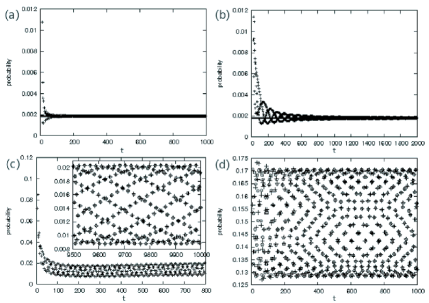
Figure 2: Comparison between theoretical values with circles and numerical estimations with crosses of $W_{t,3}$ with $C=e^{i\varphi}H$. The probability $P(X_{t,0}=1)$ is plotted. The initial state is $\psi_{0}=e^{i10\pi/180}/\sqrt{3}$, $\psi_{1}=e^{i30\pi/180}/\sqrt{3}$, $\psi_{2}=e^{i340\pi/180}/\sqrt{3}$ and (a) $\varphi=0$, (b) $\varphi=40\pi/180$, (c) $\varphi=50\pi/180$, (d) $\varphi=80\pi/180$. Since $|c|=1/\sqrt{2}$, $\varphi=45\pi/180$ is a critical point for the oscillatory behavior. In the large figure of (c), theoretical value are omitted.

From Theorem 1, the condition for the existence $L^{r}_{c}(x,t)$ is $-|c|<\cos\phi<|c|$. Therefore, in this case, the oscillation emerges when $\pi/4<\varphi<3\pi/4$. Remark that from Theorem 1 we can see the following relation,

$$\sum_{r\in\mathbb{K}_{\kappa}}L_{c}^{r}(x,t)=2b_{\kappa}^{2}\mathrm{Re}\left[\Gamma_{\times}(x,t)\left(\sum_{j\in\mathbb{K}_{\kappa}}\overline{\psi_{j}}\right)\left(\sum_{r\in\mathbb{K}_{\kappa}}\sum_{j\in\mathbb{K}_{\kappa}}(\psi_{j}-\psi_{r})\right)\right]=0,$$

This means that the oscillation disappears when we take the probability summed over all vertices with a same distance from the origin. In addition, since $P(W_{t,\kappa}=0)=\sum_{j}P(X_{t,j}=0)$, the probability of the origin does not oscillate for any condition. We also find that the distribution has an exponentially decay with $x$ from Theorem 1. The probability $P(X_{10000,0}=x)$ is shown in Fig. 3.

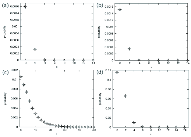
Figure 3: Comparison between theoretical values with circles and numerical estimations with crosses of $W_{t,3}$ with $C=e^{i\varphi}H$. The probability $P(X_{10000,0}=x)$ is plotted. The initial state is $\psi_{0}=e^{i10\pi/180}/\sqrt{3}$, $\psi_{1}=e^{i30\pi/180}/\sqrt{3}$, $\psi_{2}=e^{i340\pi/180}/\sqrt{3}$ and (a) $\varphi=0$, (b) $\varphi=40\pi/180$, (c) $\varphi=50\pi/180$, (d) $\varphi=80\pi/180$.

In order to state the weak convergence theorem, at first we define some parameters depending on the initial state. For $r\in\mathbb{K}_{\kappa}$, we put

$$\theta^{r}_{1}(\boldsymbol{\psi})=\left|\psi_{r}\right|^{2},$$ (3.14)

$$\theta^{r}_{2}(\boldsymbol{\psi})=\sum_{j\in{\mathbb{K}_{\kappa}}\setminus\{r\}}\overline{\psi_{r}}\psi_{j},$$ (3.15)

$$\theta^{r}_{3}(\boldsymbol{\psi})=\sum_{j\in{\mathbb{K}_{\kappa}}\setminus\{r\}}\left|\psi_{j}\right|^{2}+\sum_{j,k\in{\mathbb{K}_{\kappa}}\setminus\{r\}\atop j\neq k}\left(\psi_{j}\overline{\psi_{k}}+\overline{\psi_{j}}\psi_{k}\right).$$ (3.16)

Next, we introduce the following notations. Terms $C_{m}$ and $C^{r}_{d}$ are delta measures which are caused by localization and $C^{r}_{d}(x)$ is a weight on density function $f_{K}(x)$ which is formed a typical shape of one dimensional quantum walks.

$$C_{m}=\frac{b_{\kappa}^{2}|c|(|c|-\cos{\phi})}{2K_{-}}\left|\sum_{j\in\mathbb{K}_{\kappa}}\psi_{j}\right|^{2},\;\;C_{p}^{r}=\frac{b_{\kappa}^{2}|c|(|c|+\cos{\phi})}{2K_{+}}\left|\sum_{j\in\mathbb{K}_{\kappa}}(\psi_{j}-\psi_{r})\right|^{2},$$

$$C_{d}^{r}(x)=\frac{\Gamma_{1}(x)\theta^{r}_{1}(\boldsymbol{\psi})+2{\rm Re}(\Gamma_{2}(x)\theta^{r}_{2}(\boldsymbol{\psi}))+\Gamma_{3}(x)\theta^{r}_{3}(\boldsymbol{\psi})}{(K_{+}-(1-x^{2})\sin^{2}{\phi})(K_{-}-(1-x^{2})\sin^{2}{\phi})}x^{2},$$

$$\Gamma_{1}(x)=4a_{\kappa}|c|(|a|^{2}-x^{2})\cos{\phi}\sin^{2}{\phi}$$

$$\;\;\;\;\;\;\;\;\;\;\;\;\;\;\;\;+\left(a_{\kappa}^{2}+2a_{\kappa}|c|\cos{\phi}+1\right)\left(1+|c|^{2}-2|c|^{2}\cos^{2}{\phi}-(1-x^{2})\sin^{2}{\phi}\right),$$

$$\Gamma_{2}(x)=-2b_{\kappa}|c|(|a|^{2}-x^{2})ie^{i\phi}\cos{\phi}\sin{\phi}$$

$$\;\;\;\;\;\;\;\;\;\;\;\;\;\;\;\;+b_{\kappa}(a_{\kappa}+|c|e^{i\phi})(1+|c|^{2}-2|c|^{2}\cos^{2}{\phi}-(1-x^{2})\sin^{2}{\phi}),$$

$$\Gamma_{3}(x)=b_{\kappa}^{2}(1+|c|^{2}-2|c|^{2}\cos^{2}{\phi}-(1-x^{2})\sin^{2}{\phi}).$$

The weak convergence theorem is derived as follows.

Theorem 2 (Weak convergence)

For $\kappa\geq 1$, $r\in{\mathbb{K}_{\kappa}}$, as $t\to\infty$

$$P\left(u\leq\frac{{X_{t,r}}}{t}\leq v\right)\to\int_{u}^{v}\rho_{W}^{r}(x)dx.$$

The limit measure is defined by

$$\rho_{W}^{r}(x)=\left\{I_{[-1,|c|)}\left(\cos{\phi}\right)C_{m}+I_{(-|c|,1]}\left(\cos{\phi}\right)C_{p}^{r}\right\}\delta_{0}(x)+C_{d}^{r}(x)f_{K}(x),$$

where

$$f_{K}(x)=\frac{I_{[0,a)}(x)\sqrt{1-|a|^{2}}}{\pi(1-x^{2})\sqrt{|a|^{2}-x^{2}}}.$$

The function $C_{d}^{0}(x)f_{K}(x)$ and the scaled numerical values are shown in Fig. 4.

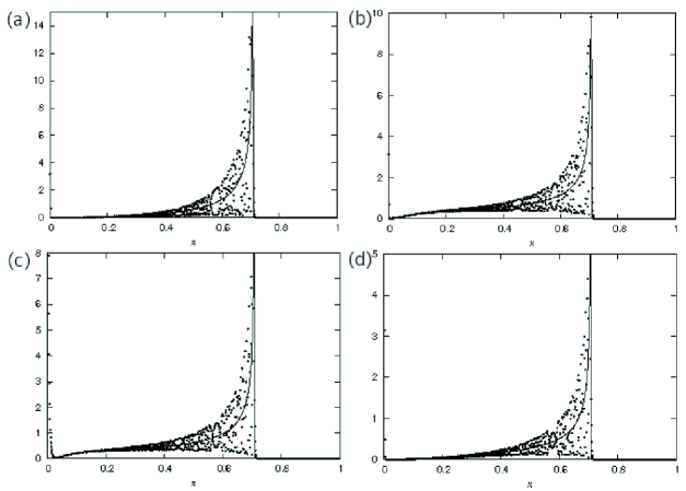
Figure 4: Comparison between theoretical values with line and numerical estimations with dots of $W_{t,3}$ with $C=e^{i\varphi}H$. Density function $C_{d}^{0}(x)f_{K}(x)$ and scaled numerical values at time $2000$ are plotted. In theoretical values, the delta measure is omitted. Since localization has an exponentially decay, the scaled numerical values corresponding to localization converge to the delta measure at the infinite time. The initial state is $\psi_{0}=e^{i10\pi/180}/\sqrt{3}$, $\psi_{1}=e^{i30\pi/180}/\sqrt{3}$, $\psi_{2}=e^{i340\pi/180}/\sqrt{3}$ and (a) $\varphi=0$, (b) $\varphi=40\pi/180$, (c) $\varphi=50\pi/180$, (d) $\varphi=80\pi/180$.

Same as other one-dimensional cases [13, 14, 15, 16, 17], this distribution has scaling order $t$ and the typical density function of quantum walks $f_{K}(x)$. The delta measures $C_{m}$ and $C^{r}_{p}$ are caused by localization, i.e., $C_{m}=\sum_{x}L_{m}(x)$ and $C^{r}_{p}=\sum_{x}L^{r}_{p}(x)$.

The above expressions of both theorems seem to be complicated, however for the following cases, they are written in simpler forms.

Corollary 3 ($\phi=0$)

For $x\in\mathbb{Z}_{+}\cup\{0\}$, $r\in{\mathbb{K}_{\kappa}}$ and $\phi=0$,

$$P({X_{t,r}}=x)\sim\\ \left(\frac{1+(-1)^{t+x}}{2}\right)\frac{b_{\kappa}^{2}|c|^{2}}{1+|c|^{2}}\left\{\delta_{0}(x)+(1-\delta_{0}(x))\left(\frac{2}{1+|c|}\right)\left(\frac{1-|c|}{1+|c|}\right)^{x-1}\right\}\left|\sum_{j\in\mathbb{K}_{\kappa}}(\psi_{j}-\psi_{r})\right|^{2},$$

and ${X_{t,r}}/t$ converges weakly to a limit measure $\rho_{W_{(0)}}^{r}$ as $t\to\infty$, where

$$\rho_{W_{(0)}}^{r}(x)=\\ \frac{b_{\kappa}^{2}|c|}{2(1+|c|)}\left|\sum_{j\in\mathbb{K}_{\kappa}}(\psi_{j}-\psi_{r})\right|^{2}\delta_{0}(x)+\frac{1}{|a|^{2}}\left(\left|(|c|-1)\psi_{r}+b_{\kappa}\sum_{j\in\mathbb{K}_{\kappa}}\psi_{j}\right|^{2}+|a|^{2}|\psi_{r}|^{2}\right)x^{2}f_{K}(x).$$

Proof.

From Theorem 1, when $\phi=0$, we have $P({X_{t,r}}=x)\sim(1+(-1)^{t+x})L_{p}^{r}(x)/2$. Also Theorem 2 implies $\Gamma_{1}(x)=|a|^{2}(a_{\kappa}^{2}+2a_{\kappa}|c|+1)$, $\Gamma_{2}(x)=|a|^{2}b_{\kappa}(a_{\kappa}+|c|)$, $\Gamma_{3}(x)=|a|^{2}b_{\kappa}^{2}$, and $K_{+}K_{-}=|a|^{4}$. After some calculations of $\theta^{r}_{1}(\boldsymbol{\psi}),\ \theta^{r}_{2}(\boldsymbol{\psi}),\ \theta^{r}_{3}(\boldsymbol{\psi})$, we have the desired conclusion. ∎

From the definition of $W_{t,\kappa}$, $W_{t,1}$ is simply a quantum walk on a half line with a reflecting wall on the origin. In the next corollary, we denote $X_{t,0}\equiv X_{t}$ to assert that the walk is defined on a half line.

Corollary 4 (Half line)

For $x\in\mathbb{Z}_{+}\cup\{0\}$,

$$P\left({X_{t}}=x\right)\sim I_{[-1,|c|)}\left(\cos{\phi}\right)\left(\frac{1+(-1)^{t+x}}{2}\right)\\ \times\frac{4|c|^{2}(\cos{\phi}-|c|)^{2}}{K_{-}^{2}}\left\{\delta_{0}(x)+(1-\delta_{0}(x))\left(\frac{|a|^{2}}{K_{-}}\right)^{x-1}\left(1+\frac{|a|^{2}}{K_{-}}\right)\right\},$$

and ${X_{t}}/t$ converges weakly to a limit measure $\rho_{X}$ as $t\to\infty$, where

$$\rho_{X}(x)=I_{[-1,|c|)}\left(\cos{\phi}\right)\frac{2|c|(|c|-\cos{\phi})}{K_{-}}\delta_{0}(x)+\frac{2(1-|c|\cos{\phi})}{K_{-}-(1-x^{2})\sin^{2}{\phi}}x^{2}f_{K}(x).$$

Proof.

For $\kappa=1$, we have $b_{1}=2/\kappa=2$, $a_{1}=b_{1}-1=1$, $\theta^{0}_{1}(\boldsymbol{\psi})=1$ and $\theta^{0}_{2}(\boldsymbol{\psi})=\theta^{0}_{3}(\boldsymbol{\psi})=0$. From Theorem 1, we get $L_{p}^{0}(x)=0$ and $L_{c}^{0}(x,t)=0$, thus we should consider only $L_{m}^{0}(x)$ as localization factor of $X_{t}$. From Theorem 2, we have $C_{p}^{0}=0$ and

$$\Gamma_{1}(x)=2(1-|c|\cos{\phi})\left\{K_{+}-(1-x^{2})\sin^{2}{\phi}\right\}.$$ (3.17)

Combining $C_{m}$ and $C_{d}^{r}(x)$ with Eq. (3.17) implies $\rho_{X}(x)$. ∎

Remark that we get another proof of Corollary 4 by considering ${W_{t,\kappa}}$ with the symmetric initial state.

We can adopt Corollary 3 for ${V_{t,\kappa}}$ with no perturbation, i.e., $\tilde{c}=1$. In $\phi=0$ case, the formula for the $r$th half line is directly expressed by $\psi_{0},\psi_{1},\ldots,\psi_{\kappa-1}$ instead of $\theta_{1}^{r}(\boldsymbol{\psi}),\theta_{2}^{r}(\boldsymbol{\psi}),\theta_{3}^{r}(\boldsymbol{\psi})$. Both cases of $\phi=0$ and half line, the oscillatory term $L_{c}^{r}(x,t)$ appearing in Theorem 1 vanishes.

4 Proofs of Theorems 1 and 2

In order to prove Theorems 1 and 2, we consider a reduction of ${W_{t,\kappa}}$ on a half line. For ${W_{t,\kappa}}$ with arbitrary initial states, we can not construct the reduction of the walk directly, since the states with the same distance from the origin have different amplitudes. To solve this problem, we introduce ${W_{t,\kappa}^{\prime}}$ which is a quantum walk with an enlarged basis of ${W_{t,\kappa}}$. After that, we construct ${X_{t}^{*}}$ as a reduction of ${W_{t,\kappa}^{\prime}}$ on a half line. To analyze ${X_{t}^{*}}$, we give the generating function of the states. By using it, we obtain the limit states and the characteristic function of ${W_{t,\kappa}}$.

4.1 Reduction to a half line

Let $\Psi_{t}(x)$ be the state of the quantum walk ${W_{t,\kappa}}$ at time $t$ and position $x$. We denote the initial state $\Psi_{0}(0)$ as $\boldsymbol{\psi}=\sum_{j\in\mathbb{K}_{\kappa}}\psi_{j}|0,\epsilon_{j}\rangle$. Now we rewrite $\boldsymbol{\psi}$ using a new orthogonal basis $\{|\epsilon_{j}^{\prime}\rangle;j\in\mathbb{K}_{\kappa}\}$ as

$$\boldsymbol{\psi}=\sum_{j\in\mathbb{K}_{\kappa}}\left(\sum_{r\in\mathbb{K}_{\kappa}}\psi_{r}\langle\epsilon^{\prime}_{r}|\otimes I_{W}\right)|\epsilon_{j}^{\prime}\rangle|0,\epsilon_{j}\rangle=\sum_{j\in\mathbb{K}_{\kappa}}\Lambda(\boldsymbol{\psi})|\epsilon_{j}^{\prime}\rangle|0,\epsilon_{j}\rangle,$$

where $I_{W}$ is the identity operator on $\mathscr{H}^{({\mathbb{J}_{\kappa}})}$ and we defined as

$$\Lambda(\boldsymbol{\psi})=\sum_{r\in{\mathbb{K}_{\kappa}}}\psi_{r}\langle{\epsilon_{r}^{\prime}}|\otimes I_{W}.$$

Now let $\mathscr{H}^{\prime}$ be a Hilbert space spanned by an orthonormal basis $\{|{{\epsilon_{j}^{\prime}}}\rangle;\ j\in{\mathbb{K}_{\kappa}}\}$. Then we define ${W_{t,\kappa}^{\prime}}$ as a quantum walk on $\mathscr{H}^{\prime}\otimes\mathscr{H}^{({\mathbb{J}_{\kappa}})}$ with the evolution operator $U_{J}^{\prime}=(I_{\kappa}\otimes S_{J})(I_{\kappa}\otimes F_{J})=I_{\kappa}\otimes U_{J}$ and the initial state $\sum_{j\in{\mathbb{K}_{\kappa}}}|{{\epsilon_{j}^{\prime}}}\rangle|{0,\epsilon_{j}}\rangle$, where $I_{\kappa}$ is the identity operator on $\mathscr{H}^{\prime}$. Let $l_{0}=\{\epsilon_{0},\epsilon_{1},\ldots,\epsilon_{\kappa-1}\}$ and $l_{x}=\{Up,Down\}$ for $x\in V({\mathbb{J}_{\kappa}})\setminus\{0\}$. Then the state of quantum walk ${W_{t,\kappa}^{\prime}}$ at time $t$ and position $x$ is written as $\Psi_{t}^{\prime}(x)=\sum_{j\in{\mathbb{K}_{\kappa}},u\in l_{x}}\alpha_{t}^{\prime}({\epsilon_{j}^{\prime}},x,u)|{{\epsilon_{j}^{\prime}}}\rangle|{x,u}\rangle$, where $\alpha^{\prime}_{t}(a,b,c)$ is the amplitude of the base $|{a,b,c}\rangle$ at time $t$. From the construction we obtain the following lemma.

Lemma 2 (Enlarging basis)

For any $t\geq 0$ and $x\in V({\mathbb{J}_{\kappa}})$,

$$\Psi_{t}(x)=\Lambda(\boldsymbol{\psi})\Psi_{t}^{\prime}(x).$$

Proof.

We show the equation by induction with respect to $t$. At $t=0$, by definition of $\Lambda(\boldsymbol{\psi})$, it is trivial. For fixed $t\geq 1$, we assume $\Psi_{t}(x)=\Lambda(\boldsymbol{\psi})\Psi_{t}^{\prime}(x)$, then for $x\in V({\mathbb{J}_{\kappa}})$,

$$U_{J}^{\prime}\Psi^{\prime}_{t}(x) = (I_{\kappa}\otimes U_{J})\sum_{j\in{\mathbb{K}_{\kappa}},u\in l_{x}}\alpha_{t}^{\prime}({\epsilon_{j}^{\prime}},x,u)|{{\epsilon_{j}^{\prime}}}\rangle|{x,u}\rangle$$

$$= \sum_{j\in{\mathbb{K}_{\kappa}},u\in l_{x}}\alpha_{t}^{\prime}({\epsilon_{j}^{\prime}},x,u)|{{\epsilon_{j}^{\prime}}}\rangle\left(U_{J}|{x,u}\rangle\right),$$

$$U_{J}\Psi_{t}(x) = U_{J}\Lambda(\boldsymbol{\psi})\Psi_{t}^{\prime}(x)$$

$$= U_{J}\Lambda(\boldsymbol{\psi})\sum_{j\in{\mathbb{K}_{\kappa}},u\in l_{x}}\alpha_{t}^{\prime}({\epsilon_{j}^{\prime}},x,u)|{{\epsilon_{j}^{\prime}}}\rangle|{x,u}\rangle$$

$$= U_{J}\sum_{j\in{\mathbb{K}_{\kappa}},u\in l_{x}}\psi_{j}^{\prime}\alpha_{t}^{\prime}({\epsilon_{j}^{\prime}},x,u)|{x,u}\rangle$$

$$= \sum_{j\in{\mathbb{K}_{\kappa}},u\in l_{x}}\psi_{j}^{\prime}\alpha_{t}^{\prime}({\epsilon_{j}^{\prime}},x,u)U_{J}|{x,u}\rangle$$

$$= \Lambda(\boldsymbol{\psi})\sum_{j\in{\mathbb{K}_{\kappa}},u\in l_{x}}\alpha_{t}^{\prime}({\epsilon_{j}^{\prime}},x,u)|{{\epsilon_{j}^{\prime}}}\rangle\left(U_{J}|{x,u}\rangle\right)$$

$$= \Lambda(\boldsymbol{\psi})U^{\prime}_{J}\Psi^{\prime}_{t}(x).$$

This relation holds for any $x$, so we conclude $\Psi_{t+1}(x)=\Lambda(\boldsymbol{\psi})\Psi_{t+1}^{\prime}(x)$. ∎

For $x\in V({\mathbb{J}_{\kappa}})$, we define the probability of “${W_{t,\kappa}^{\prime}}=x$” by $P({W_{t,\kappa}^{\prime}}=x)=\|\Lambda(\boldsymbol{\psi})\Psi_{t}^{\prime}(x)\|^{2}$. Then it follows form Lemma 2 that $P({W_{t,\kappa}^{\prime}}=x)=P({W_{t,\kappa}}=x)$ for any $x\in V({\mathbb{J}_{\kappa}})$. For ${W_{t,\kappa}^{\prime}}$, the information of the initial state is covered by $\Lambda(\boldsymbol{\psi})$. In other words, for any initial state of ${W_{t,\kappa}}$, it is enough to consider the initial state $\sum_{j\in{\mathbb{K}_{\kappa}}}|{{\epsilon_{j}^{\prime}}}\rangle|{0,\epsilon_{j}}\rangle$ on ${W_{t,\kappa}^{\prime}}$. Consequently, the states of the quantum walk ${W_{t,\kappa}^{\prime}}$ have a good symmetry, so we can treat the reduction of the walk.

Now we introduce ${X_{t}^{*}}$ as a reduction of ${W_{t,\kappa}^{\prime}}$ on a half line. Here ${X_{t}^{*}}$ is defined on a Hilbert space generated by the following new basis. For all $l\in\{Up,Down\}$ and $x\in\mathbb{Z}_{+}$,

$$|{Own,0,\epsilon}\rangle=\sum_{j\in{\mathbb{K}_{\kappa}}}|{{\epsilon_{j}^{\prime}},0,\epsilon_{j}}\rangle,$$

$$|{Other,0,\epsilon}\rangle=\frac{1}{\sqrt{\kappa-1}}\sum_{j\in{\mathbb{K}_{\kappa}}}\sum_{k\in{\mathbb{K}_{\kappa}}\setminus\{j\}}|{{\epsilon_{k}^{\prime}},0,\epsilon_{j}}\rangle,$$

$$|{Own,x,l}\rangle=\sum_{j\in{\mathbb{K}_{\kappa}}}|{{\epsilon_{j}^{\prime}},{h_{j}}(x),l}\rangle,$$

$$|{Other,x,l}\rangle=\frac{1}{\sqrt{\kappa-1}}\sum_{j\in{\mathbb{K}_{\kappa}}}\sum_{k\in{\mathbb{K}_{\kappa}}\setminus\{j\}}|{{\epsilon_{k}^{\prime}},{h_{j}}(x),l}\rangle.$$

On this basis, we obtain the one-step time evolution. For $x\in\mathbb{Z}_{+}$,

$$U_{J}^{\prime}\ :\ \begin{array}[]{l}|{Own,0,\epsilon}\rangle\to a_{\kappa}|{Own,1,Down}\rangle+\sqrt{\kappa-1}b_{\kappa}|{Other,1,Down}\rangle,\\ |{Other,0,\epsilon}\rangle\to\sqrt{\kappa-1}b_{\kappa}|{Own,1,Down}\rangle-a_{\kappa}|{Other,1,Down}\rangle,\\ |{Own,x,Up}\rangle\to a|{Own,x-1,Up}\rangle+c|{Own,x+1,Down}\rangle,\\ |{Other,x,Up}\rangle\to a|{Other,x-1,Up}\rangle+c|{Other,x+1,Down}\rangle,\\ |{Own,x,Down}\rangle\to b|{Own,x-1,Up}\rangle+d|{Own,x+1,Down}\rangle,\\ |{Other,x,Down}\rangle\to b|{Other,x-1,Up}\rangle+d|{Other,x+1,Down}\rangle.\end{array}$$

The subspace generated by this basis is invariant under the operation $U_{J}^{\prime}$. Moreover the initial state of ${W_{t,\kappa}^{\prime}}$ can be written as $|{Own,0,\epsilon}\rangle$. Therefore we can write the evolution operator of ${X_{t}^{*}}$ as $U_{H}^{*}=F_{H}^{*}S_{H}^{*}$. The coin operator $F_{H}^{*}$ is defined by

$$F_{H}^{*}=\left[\begin{array}[]{cc}a_{\kappa}&\sqrt{\kappa-1}b_{\kappa}\\ \sqrt{\kappa-1}b_{\kappa}&-a_{\kappa}\\ \end{array}\right]\otimes|{0}\rangle\langle{0}|\otimes 1+\sum_{x\in\mathbb{Z}_{+}}I_{2}\otimes|{x}\rangle\langle{x}|\otimes C.$$

For $m\in\{Own,Other\}$, $l\in\{Up,Down\}$, the shift operator $S^{*}$ is defined by

$$S_{H}^{*}|{m,0,\epsilon}\rangle=|{m,1,Down}\rangle,$$

$$S_{H}^{*}|{m,1,l}\rangle=\left\{\begin{array}[]{ll}|{m,0,\epsilon}\rangle,&l=Up,\\ |{m,2,Down}\rangle,&l=Down,\\ \end{array}\right.$$

$$S_{H}^{*}|{m,x,l}\rangle=\left\{\begin{array}[]{ll}|{m,x-1,Up}\rangle,&l=Up,\\ |{m,x+1,Down}\rangle,&l=Down,\\ \end{array}\right.\ x\geq 2.$$

Throughout this paper, we put $|{Own}\rangle={}^{T}[1,0]$ and $|{Other}\rangle={}^{T}[0,1]$. An expression of ${X_{t}^{*}}$ using weights is shown by Fig. 5 and Eqs. (.45)-(.55) in Appendix.

Let $\Psi_{t}^{*}(x)$ be the state of the quantum walk ${X_{t}^{*}}$. Now we define for $r\in{\mathbb{K}_{\kappa}}$,

$$\Lambda_{r}(\boldsymbol{\psi})=\left(\psi_{r}\langle{Own}|+\sqrt{\kappa-1}\sum_{j\in{\mathbb{K}_{\kappa}}\setminus\{r\}}\psi_{j}\langle{Other}|\right)\otimes I_{W}.$$

Then we introduce ${X_{t,r}}$ whose probability of “${X_{t,r}}=x$” is defined by

$$P({X_{t,r}}=x)=\|\Lambda_{r}(\boldsymbol{\psi})\Psi_{t}^{*}(x)\|^{2}.$$ (4.22)

This probability is described by the state of $W_{t,\kappa}$ in the following,

$$P({X_{t,r}}=x)=\left\{\begin{array}[]{ll}|\alpha_{t}(0,\epsilon_{r})|^{2},&x=0,\\ \|\Psi_{t}({h_{r}}(x))\|^{2},&\mathrm{otherwise.}\\ \end{array}\right.$$

Hence the relation between the probabilities of “${W_{t,\kappa}}={h_{r}}(x)$” and “${X_{t,r}}=x$” is obtained as

$$P({W_{t,\kappa}}={h_{r}}(x))=\left\{\begin{array}[]{ll}\sum\limits_{j\in{\mathbb{K}_{\kappa}}}P(X_{t,j}=0),&x=0,\\ P({X_{t,r}}=x),&\mathrm{otherwise.}\\ \end{array}\right.$$

Note that $\sum_{j\in{\mathbb{K}_{\kappa}}}\sum_{x\in\{0\}\cup\mathbb{Z}_{+}}P(X_{t,j}=x)=1$.

In Subsections 4.2 and 4.3, we analyze $\Psi_{t}^{*}(x)$ by the generating function.

4.2 Proof of Theorem 1

We compute the limit state of ${X_{t}^{*}}$ from the generating function which is defined by

$$\tilde{\Psi}^{*}(x;z)=\sum_{t=0}^{\infty}\Psi_{t}^{*}(x)z^{t}=\sum_{\begin{subarray}{c}l\in\{Own,Other\}\\ m\in\{Up,Down\}\end{subarray}}\tilde{\alpha}^{*}(l,x,m;z)|{l,x,m}\rangle.$$

From Appendix, we see that there exists $0<r_{1}<1$ so that for any $z$ with $|z|<r_{1}$,

$$\tilde{\alpha}^{*}(Own,x,Up;z)=\left\{\begin{array}[]{ll}-\frac{d}{ac}(\lambda(z)-az)(\mu(z)+a_{\kappa})\Phi(x;z),&x>0,\\ -(\mu(z)+a_{\kappa})\mu(z)\Phi(x;z),&x=0,\end{array}\right.$$ (4.27)

$$\tilde{\alpha}^{*}(Other,x,Up;z)=\left\{\begin{array}[]{ll}-\frac{d\sqrt{\kappa-1}}{ac}(\lambda(z)-az)b_{\kappa}\Phi(x;z),&x>0,\\ -\sqrt{\kappa-1}b_{\kappa}\mu(z)\Phi(x;z),&x=0,\end{array}\right.$$ (4.30)

$$\tilde{\alpha}^{*}(Own,x,Down;z)=\left\{\begin{array}[]{ll}-z(\mu(z)+a_{\kappa})\Phi(x;z),&x>0,\\ 0,&x=0,\end{array}\right.$$ (4.33)

$$\tilde{\alpha}^{*}(Other,x,Down;z)=\left\{\begin{array}[]{ll}-z\sqrt{\kappa-1}b_{\kappa}\Phi(x;z),&x>0,\\ 0,&x=0,\end{array}\right.$$ (4.36)

$$\Phi(x;z)=\left\{\frac{d\lambda(z)}{a}\right\}^{x-1}\frac{w_{+}^{2}w_{-}^{2}\left(\eta_{+}(z)+\sqrt{\nu(z)}\right)\left(\eta_{-}(z)-\sqrt{\nu(z)}\right)}{4(1-c^{2})(z^{2}-w_{+}^{2})(z^{2}-w_{-}^{2})},$$ (4.37)

where

$$\lambda(z)=\frac{\Delta z^{2}+1-\sqrt{\Delta^{2}z^{4}+2\Delta(1-2|a|^{2})z^{2}+1}}{2dz},$$

$$\mu(z)=\frac{d\lambda(z)-\Delta z}{c}z,$$

$$\nu(z)=(1+\Delta z^{2})^{2}-4\Delta|a|^{2}z^{2},$$

$$\eta_{\pm}(z)=2c\pm 1\mp\Delta z^{2},$$

$$w_{\pm}^{2}=\mp\frac{c(1\pm c)}{\Delta(|a|^{2}-1\mp c)},$$

$$\Delta=ad-bc.$$

Note that $|w_{\pm}^{2}|=\left|(1\pm c)/(\overline{1\pm c})\right|=1$. From Cauchy’s theorem, we have for $0<r<r_{1}<1$,

$$\Psi_{t}^{*}(x)=\frac{1}{2\pi i}\oint_{|z|=r}\tilde{\Psi}^{*}(x;z)\frac{dz}{z^{t+1}}.$$

Therefore as $t\to\infty$

$$-\Psi_{t}^{*}(x)\sim{\rm Res}(\tilde{\Psi^{*}}(x;z),w_{+})w_{+}^{-(t+1)}+{\rm Res}(\tilde{\Psi^{*}}(x;z),-w_{+})(-w_{+})^{-(t+1)}\\ +{\rm Res}(\tilde{\Psi^{*}}(x;z),w_{-})w_{-}^{-(t+1)}+{\rm Res}(\tilde{\Psi^{*}}(x;z),-w_{-})(-w_{-})^{-(t+1)},$$

where ${\rm Res}(f(z),w)$ is the residue of $f(z)$ for $z=w$. Taking the residues of the generating function, we can compute $\Psi_{t}^{*}(x)$. After some calculations with Eq.(9) and $\Psi^{*}_{t}(x)$, the proof of Theorem 1 is complete.

4.3 Proof of Theorem 2

In order to prove Theorem 2, we calculate the Fourier transform of the generating function as $\hat{\tilde{\Psi}}^{*}(s;z)=\sum_{x}\tilde{\Psi}^{*}(x;z)e^{isx}$ by Eqs. (4.27)-(4.36). Then we obtain the characteristic function from the following relation

$$E\left[e^{i\xi{X_{t,r}}}\right] = \sum_{x\in\mathbb{Z}}\langle\Lambda_{r}(\boldsymbol{\psi})\Psi_{t}^{*}(x),\Lambda_{r}(\boldsymbol{\psi})\Psi_{t}^{*}(x)\rangle e^{i\xi x}$$ (4.38)

$$= \sum_{x,y\in\mathbb{Z}}\langle\Lambda_{r}(\boldsymbol{\psi})\Psi_{t}^{*}(x),\Lambda_{r}(\boldsymbol{\psi})\Psi_{t}^{*}(y)\rangle e^{i\xi x}\int_{0}^{2\pi}e^{ik(x-y)}\frac{dk}{2\pi}$$

$$= \int_{0}^{2\pi}\left\{\sum_{x,y\in\mathbb{Z}}\langle\Lambda_{r}(\boldsymbol{\psi})\Psi_{t}^{*}(x),\Lambda_{r}(\boldsymbol{\psi})\Psi_{t}^{*}(y)\rangle e^{ik(x-y)}e^{i\xi x}\right\}\frac{dk}{2\pi}$$

$$= \int_{0}^{2\pi}\langle\Lambda_{r}(\boldsymbol{\psi})\hat{\Psi}_{t}^{*}(s),\Lambda_{r}(\boldsymbol{\psi})\hat{\Psi}_{t}^{*}(s+\xi)\rangle\frac{ds}{2\pi},$$

where $\langle\boldsymbol{u},\boldsymbol{v}\rangle$ is the inner product of vectors $\boldsymbol{u}$ and $\boldsymbol{v}$.

Now we write the Fourier transform of the generating function as

$$\hat{\tilde{\Psi}}^{*}(s;z)=\sum_{\scriptsize{\begin{matrix}l\in\{Own,Other\}\\ m\in\{Up,Down\}\end{matrix}}}\hat{\tilde{\alpha}}^{*}(l,m;s;z)|{l,m}\rangle.$$

From Eqs. (4.27)-(4.36), we have $\hat{\tilde{\Psi}}^{*}(s;z)$ as

$$\hat{\tilde{\alpha}}^{*}(Own,Up;s;z)=\left(-\mu(z)+\frac{d}{ac}(\lambda(z)-az)\Phi_{2}(s;z)\right)(a_{\kappa}+\mu(z))\Phi_{1}(s;z),$$

$$\hat{\tilde{\alpha}}^{*}(Own,Down;s;z)=\left(-\mu(z)+\frac{d}{ac}(\lambda(z)-az)\Phi_{2}(s;z)\right)\sqrt{\kappa-1}b_{\kappa}\Phi_{1}(s;z),$$

$$\hat{\tilde{\alpha}}^{*}(Other,Up;s;z)=z(a_{\kappa}+\mu(z))\Phi_{1}(s;z)\Phi_{2}(s;z),$$

$$\hat{\tilde{\alpha}}^{*}(Other,Down;s;z)=z\sqrt{\kappa-1}b_{\kappa}\Phi_{1}(s;z)\Phi_{2}(s;z),$$

where

$$\Phi_{1}(s;z)=\frac{w_{+}^{2}w_{-}^{2}}{4(1-c^{2})}\frac{\left(\eta_{+}(z)+\sqrt{\nu(z)}\right)\left(\eta_{-}(z)-\sqrt{\nu(z)}\right)}{(z^{2}-w_{+}^{2})(z^{2}-w_{-}^{2})},$$

$$\Phi_{2}(s;z)=\frac{e^{ik}\left(\zeta(s;z)-\sqrt{\nu(z)}\right)}{2\Delta(z-v_{+}(s))(z-v_{-}(s))},$$

$$\zeta(s;z)=2ae^{-is}z-1-\Delta z^{2},$$

$$v_{\pm}(s)=\frac{ae^{-is}+\overline{a}\Delta e^{is}\pm\sqrt{(ae^{-is}+\overline{a}\Delta e^{is})^{2}-4\Delta}}{2\Delta}.$$

Here we can rewrite $v_{\pm}(s)$ as

$$v_{\pm}(s)=e^{-i\rho}(|a|\cos{\gamma(s)}\pm\sqrt{|a|^{2}\cos^{2}{\gamma(s)}-1})=e^{-i\rho}e^{\pm i\theta(s)},$$

where we take $\Delta=e^{2i\rho}$, $a=|a|e^{i\sigma}$, $\gamma(s)=s-\sigma+\rho$, $\cos{\theta(s)}=|a|\cos{\gamma(s)}$. Note that $|v_{\pm}(s)|=1$. Now $||\hat{\tilde{\Psi}}^{*}(s;z)||^{2}<\infty$ for $0<|z|<r_{1}$, we can rewrite $\hat{\tilde{\Psi}}^{*}(s;z)=\sum_{t\geq 0}\hat{\Psi}^{*}_{t}(s)z^{t}$. So we have for $0<r<r_{1}$

$$\hat{\Psi}_{t}^{*}(s)=\frac{1}{2\pi i}\oint_{|z|=r}\hat{\tilde{\Psi}}(s;z)\frac{dz}{z^{t+1}}.$$

Therefore we get the Fourier transform of the state $\hat{\Psi}_{t}^{*}(s)$ as follows:

$$-\hat{\Psi}_{t}^{*}(s)\sim\psi_{w_{+}}(s)(w_{+})^{-(t+1)}+\psi_{-w_{+}}(s)(-w_{+})^{-(t+1)}\\ \hskip 42.67912pt+\psi_{w_{-}}(s)(w_{-})^{-(t+1)}+\psi_{-w_{-}}(s)(-w_{-})^{-(t+1)}\\ \hskip 42.67912pt+\psi_{v_{+}}(s)(v_{+}(s))^{-(t+1)}+\psi_{v_{-}}(s)(v_{-}(s))^{-(t+1)},$$ (4.39)

where $\psi_{\pm w_{\pm}}(s)={\rm Res}(\hat{\tilde{\Psi}}(s;z);\pm w_{\pm})$ and $\psi_{v_{\pm}}(s)={\rm Res}(\hat{\tilde{\Psi}}(s;z);v_{\pm}(s))$.

Finally we compute the characteristic function by Eqs.(4.38) and (4.39). Now we have

$$\int_{0}^{2\pi}\left(\|\Lambda_{r}(\boldsymbol{\psi})\psi_{w_{+}}(s)\|^{2}+\|\Lambda_{r}(\boldsymbol{\psi})\psi_{-w_{+}}(s)\|^{2}\right)\frac{ds}{2\pi}=C_{p}^{r},$$

$$\int_{0}^{2\pi}\left(\|\Lambda_{r}(\boldsymbol{\psi})\psi_{w_{-}}(s)\|^{2}+\|\Lambda_{r}(\boldsymbol{\psi})\psi_{-w_{-}}(s)\|^{2}\right)\frac{ds}{2\pi}=C_{m},$$

$$\int_{0}^{2\pi}\left(\langle\Lambda_{r}(\boldsymbol{\psi})\psi_{w_{+}}(s),\Lambda_{r}(\boldsymbol{\psi})\psi_{-w_{+}}(s)\rangle+\langle\Lambda_{r}(\boldsymbol{\psi})\psi_{-w_{+}}(s),\Lambda_{r}(\boldsymbol{\psi})\psi_{w_{+}}(s)\rangle\right)\frac{ds}{2\pi}=0,$$

$$\int_{0}^{2\pi}\left(\langle\Lambda_{r}(\boldsymbol{\psi})\psi_{w_{-}}(s),\Lambda_{r}(\boldsymbol{\psi})\psi_{-w_{-}}(s)\rangle+\langle\Lambda_{r}(\boldsymbol{\psi})\psi_{-w_{-}}(s),\Lambda_{r}(\boldsymbol{\psi})\psi_{w_{-}}(s)\rangle\right)\frac{ds}{2\pi}=0.$$

Noting that $e^{i(t+1)\theta(s+\xi/t)}=e^{i(t+1)\theta(s)+i\xi h(s)+o(t^{-1})}$, where $h(s)=d\theta(s)/ds$, the above equation and Eq.(4.38) with the Riemann-Lebesgue lemma imply

$$\lim_{t\to\infty}E\left[e^{i\xi{X_{t,r}}/t}\right]=C_{p}^{r}+C_{m}+\int_{0}^{2\pi}e^{-i\xi h(s)}p(s)\frac{ds}{2\pi}+\int_{0}^{2\pi}e^{i\xi h(s)}q(s)\frac{ds}{2\pi},$$ (4.40)

where $p(s)=\|\Lambda_{r}(\boldsymbol{\psi})\psi_{v_{+}}(s)\|^{2}$ and $q(s)=\|\Lambda_{r}(\boldsymbol{\psi})\psi_{v_{-}}(s)\|^{2}$. Moreover, from a change of variable for last two terms in Eq. (4.40), we have

$$\int_{0}^{2\pi}\left(e^{-i\xi h(s)}p(s)+e^{i\xi h(s)}q(s)\right)\frac{ds}{2\pi}=\int_{0}^{\infty}e^{i\xi x}w(x)f_{K}(x)dx.$$

After some calculations for $w(x)$ with $p(s)$ and $q(s)$, we have the desired conclusion.

5 Summary and discussions

We introduced a quantum walk with an enlarged basis to consider a reduction of quantum walks with arbitrary initial state. This method is based on an idea canceling the asymmetry caused from initial state by a new tensor product. From our results in this paper, we discuss two interesting points. First, we found the oscillating probability as localization. From Theorem 1, the oscillatory term is expressed by $L_{c}^{r}(x,t)$. We can see that this term vanishes with some initial states or local coins. For example, we consider ${V_{t,\kappa}}$, which is a quantum walk on $\mathbb{T}_{\kappa}$ with local coin operators $G_{\kappa}$ with additional complex phase $\tilde{c}$ at the origin. If $\tilde{c}=1$ Corollary 3 implies that the oscillation does not occur with arbitrary initial state. Also if the initial state is symmetric, the walk is reduced on a half line. Then it follows from Corollary 4 that no oscillatory behavior arise with any complex phase $\tilde{c}$. Thus the initial state and differences on complex phase of local coins are important factors for the oscillatory behavior on localization. Especially in quantum walks on the one-dimensional lattice with homogeneous local coins, localization does not occur [13, 14, 15]. If localization occurs with perturbations of local coin operators on the one-dimensional lattice, there seems to be a condition that an oscillatory behavior arises in localization. Second, ${W_{t,\kappa}}$ has the scaling order $t$ and the limit measure has the density function $f_{K}(x)$ which is a half-line version of one appearing in the quantum walk on a line [13, 14, 15]. This is a typical property of quantum walks [8, 16, 17]. To show the universality of the limit theorems for quantum walks is one of the interesting future’s problems.

Acknowledgments. We thank Noriko Saitoh and Jun Kodama for useful discussions. N.K. is supported by the Grant-in-Aid for Scientific Research (C) (No. 21540118).

Appendix

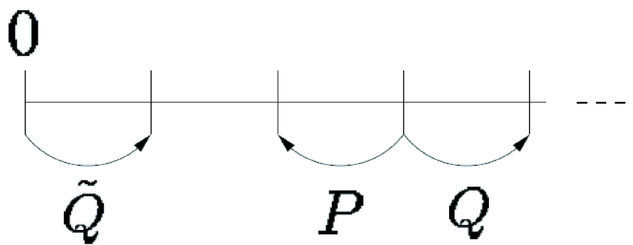
Figure 5: Quantum walk with enlarged bases ${X_{t}^{*}}$ on a half line

We calculate the generating function of $\Psi_{t}^{*}(x)$ by using the method in [23]. To simplify notations, for $l\in\{Own,Other\}$, we denote $|l,0,\epsilon\rangle=|l,0,Up\rangle$ and construct $|l,0,Down\rangle$ as a dummy base, which always has value $0$ as its amplitude, so that the local coin operator on the origin has $2\times 2$ matrix. To indicate the evolution operator of the walk, we use an expression using weights (see Fig.5), where

$$\tilde{Q}=\left[\begin{array}[]{cc}a_{\kappa}&\sqrt{\kappa-1}b_{\kappa}\\ \sqrt{\kappa-1}b_{\kappa}&-a_{\kappa}\\ \end{array}\right]\otimes\left[\begin{array}[]{cc}0&0\\ 1&0\\ \end{array}\right],$$ (.45)

$$P=I_{2}\otimes\left[\begin{array}[]{cc}a&b\\ 0&0\\ \end{array}\right]\ ,\ Q=I_{2}\otimes\left[\begin{array}[]{cc}0&0\\ c&d\\ \end{array}\right],$$ (.50)

$$\Psi_{0}^{*}(0)=\left[\begin{array}[]{c}1\\ 0\\ \end{array}\right]\otimes\left[\begin{array}[]{c}1\\ 0\\ \end{array}\right].$$ (.55)

We define the generating function for the state by

$$\tilde{\Psi}^{*}(x;z)=\sum_{t=0}^{\infty}\Psi_{t}^{*}(x)z^{t}.$$

In order to compute $\tilde{\Psi}^{*}(x;z)$, we first define the transition amplitude $\tilde{\Xi}(0\to x;\tau)$ as the weight of all paths starting from $0$ ending at $x$ after $\tau$ steps, and $\Xi(0\to x;\tau)$ as the weight of all paths on another walk defined by $Q_{0}^{\prime}=Q$. For example, $\tilde{\Xi}(0\to 2;4)=QPQ\tilde{Q}+PQQ\tilde{Q}+Q\tilde{Q}P\tilde{Q}$ and $\Xi(0\to 2;4)=QPQQ+PQQQ+QQPQ$. From $\tilde{\Xi}(0\to 0;\tau_{1})$ and $\Xi(0\to x-1;\tau_{2})$, we can obtain $\tilde{\Xi}(0\to x;\tau_{1}+\tau_{2}+1)$ as Fig.6. Then we get $\tilde{\Psi}^{*}(x;z)$ from the generating function for $\tilde{\Xi}(0\to x;\tau)$.

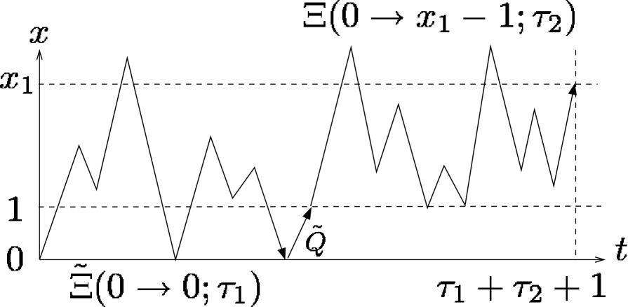
Figure 6: $\tilde{\Xi}(0\to x_{1};\tau_{1}+\tau_{2}+1)$

We now calculate the generating function for $\Xi(0\to x;\tau)$. Since the first operator should be $Q$ on the half line, the weights of paths form $Q\cdots Q$ or $P\cdots Q$. So we express $\Xi(0\to x;\tau)$ as a linear combination of $Q$ and $R$:

$$\Xi(0\to x;\tau)=b^{q}(0\to x;\tau)Q+b^{r}(0\to x;\tau)R+\delta_{0}(x)\delta_{0}(\tau)I_{2}\otimes I_{2}$$

where $R=I_{2}\otimes\left[\begin{array}[]{cc}c&d\\ 0&0\\ \end{array}\right]$ and we define $b^{q}(0\to x;0)=b^{r}(0\to x;0)=0$. The generating function for $\Xi(0\to x;\tau)$ is defined by

$$\sum_{\tau=0}^{\infty}\Xi(0\to x;\tau)z^{\tau}=B^{q}(0\to x;z)Q+B^{r}(0\to x;z)R+\delta_{0}(x)I_{2}\otimes I_{2},$$

with $B^{q}(0\to x;z)=\sum_{\tau=0}^{\infty}b^{q}(0\to x;\tau)z^{\tau}$ and $B^{r}(0\to x;z)=\sum_{\tau=0}^{\infty}b^{r}(0\to x;\tau)z^{\tau}$. Since the left-hand tensor product of $P$ and $Q$ is $I_{2}$, the generating function for $\Xi(0\to x;\tau)$ corresponds to the result in [23], i.e., for sufficiently small $z$,

$$B^{q}(0\to x;z)=\left\{\frac{d}{a}\lambda(z)\right\}^{x}\frac{1}{d},\ x\geq 1,$$

$$B^{q}(0\to 0;z)=0,$$

$$B^{r}(0\to x;z)=\left\{\frac{d}{a}\lambda(z)\right\}^{x}\frac{\lambda(z)-az}{acz},\ x\geq 0,$$

$$\lambda(z)=\frac{\Delta z^{2}+1-\sqrt{\Delta^{2}z^{4}+2\Delta(1-2|a|^{2})z^{2}+1}}{2dz}.$$ (.56)

Here we take $\lambda(z)$ for the smaller solution of the absolute value of

$$\lambda^{2}(z)-\frac{1}{d}\left(\Delta z+\frac{1}{z}\right)\lambda(z)+\frac{a}{d}=0.$$ (.57)

Note that for sufficiently small $z$ we can write $\lambda(z)$ by Eq. (.56). Moreover since $|a/d|=1$, we can take $r_{0}<1$ such that $|\lambda(z)|<1$ for $|z|<r_{0}$. Next we calculate the generating function for $\tilde{\Xi}(0\to 0;\tau)$. To do so, we introduce a new notation $\tilde{\Xi}(0\to 0;\tau;n)$ as the weight of all paths starting from the origin reaching the origin $n$ times before ending at the origin at time $\tau$. Now we consider $\tilde{\Xi}(0\to 0;\tau;0)$. For $\tau\geq 2$, we obtain $\tilde{\Xi}(0\to 0;\tau;0)$ as (see Fig.7)

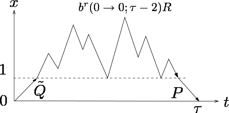
Figure 7: $\tilde{\Xi}(0\to 0;\tau;0)$

$$\tilde{\Xi}(0\to 0;\tau;0) = (1-\delta_{2}(\tau))P\{b^{r}(0\to 0;\tau-2)R\}\tilde{Q}+\delta_{2}(\tau)P\tilde{Q}$$

$$= \{(1-\delta_{2}(\tau))abb^{r}(0\to 0;\tau-2)+\delta_{2}(\tau)b\}\tilde{R},$$

where $\tilde{R}=\left[\begin{array}[]{cc}a_{\kappa}&\sqrt{\kappa-1}b_{\kappa}\\ \sqrt{\kappa-1}b_{\kappa}&-a_{\kappa}\\ \end{array}\right]\otimes\left[\begin{array}[]{cc}1&0\\ 0&0\\ \end{array}\right]$ and for $\tau<2$ we define $\tilde{\Xi}(0\to 0;\tau;0)=0$. Therefore we get the generating function for $\tilde{\Xi}(0\to 0;\tau;0)$ as

$$\sum_{\tau=0}^{\infty}\tilde{\Xi}(0\to 0;\tau;0)z^{\tau}=(adB^{r}(0\to 0;z)+b)z^{2}\tilde{R}=B^{\tilde{r}}(0\to 0;z;0)\tilde{R}.$$

Similarly, for $\tau\geq 4$ we have $\tilde{\Xi}(0\to 0;\tau;1)$ as

$$\tilde{\Xi}(0\to 0;\tau;1)=\sum_{\tau_{1}+\tau_{2}+4=\tau}\{(1-\delta_{2}(\tau_{1}))abb^{r}(0\to 0;\tau_{1})+\delta_{2}(\tau_{1})b\}\tilde{R}\\ \times\{(1-\delta_{2}(\tau_{2}))abb^{r}(0\to 0;\tau_{2})+\delta_{2}(\tau_{2})b\}\tilde{R},$$

and for $\tau<4$ we define $\tilde{\Xi}(0\to 0;\tau;1)=0$. Thus the generating function for $\tilde{\Xi}(0\to 0;\tau;1)$ is obtained by

$$\sum_{\tau=0}^{\infty}\tilde{\Xi}(0\to 0;\tau;1)z^{\tau}=\{(adB^{r}(0\to 0;z)+b)z^{2}\}^{2}\tilde{R}_{I}=B^{\tilde{r}_{I}}(0\to 0;z;1)\tilde{R}_{I},$$

where $\tilde{R}_{I}=I_{2}\otimes\left[\begin{array}[]{cc}1&0\\ 0&0\\ \end{array}\right]$. Recursively we have the following formulae: for $n\geq 0$,

$$B^{\tilde{r}}(0\to 0;z;n)=\left(\frac{1+(-1)^{n}}{2}\right)\{(adB^{r}(0\to 0;z)+b)z^{2}\}^{n+1},$$ (.58)

$$B^{\tilde{r}_{I}}(0\to 0;z;n)=\left(\frac{1+(-1)^{n+1}}{2}\right)\{(adB^{r}(0\to 0;z)+b)z^{2}\}^{n+1}.$$ (.59)

From Eqs. (.58) and (.59), we get the generation function for $\tilde{\Xi}(0\to 0;\tau)$ by summing over $n$. Here $(dB^{r}(0\to 0;z)-\Delta z)z^{2}=(d\lambda(z)-\Delta z)z/c$, so we see that for $z$ with $|z|<r_{1}\equiv{\rm min}(|c|,r_{0})$,

$$|(d\lambda(z)-\Delta z)z/c|^{2}\leq(|d\lambda(z)|^{2}+|z|^{2})|z/c|^{2}<|d|^{2}+|c|^{2}=1.$$

Therefore for $z$ such that $|z|<r_{1}$,

$$\sum_{\tau=0}^{\infty}\tilde{\Xi}(0\to 0;\tau)z^{\tau}=B^{\tilde{r}}(0\to 0;z)\tilde{R}+B^{\tilde{r}_{I}}(0\to 0;z)\tilde{R}_{I}+I_{2}\otimes I_{2},$$

$$B^{\tilde{r}}(0\to 0;z)=\sum_{n=0}^{\infty}B^{\tilde{r}}(0\to 0;z;n)=\frac{(d\lambda(z)-\Delta z)z/c}{1-\{\tilde{c}(d\lambda(z)-\Delta z)z/c\}^{2}},$$

$$B^{\tilde{r}_{I}}(0\to 0;z)=\sum_{n=0}^{\infty}B^{\tilde{r}_{I}}(0\to 0;z;n)=\frac{\{(d\lambda(z)-\Delta z)z/c\}^{2}}{1-\{(d\lambda(z)-\Delta z)z/c\}^{2}}.$$

For $x\geq 1$, $\tilde{\Xi}(0\to x;\tau)$ is written by $\tilde{\Xi}(0\to 0;\tau)$ and $\Xi(0\to x;\tau)$ (see Fig.6) as

$$\tilde{\Xi}(0\to x;\tau)=\sum_{\tau_{1}+\tau_{2}+1=\tau}\Xi(0\to x-1;\tau_{2})\tilde{Q}\tilde{\Xi}(0\to 0;\tau_{1})+\delta_{0}(\tau)\delta_{0}(x)I_{2}\otimes I_{2}.$$

From the generating function for $\tilde{\Xi}(0\to 0;\tau)$ and $\Xi(0\to x;\tau)$, we can compute the generating function for $\tilde{\Xi}(0\to x;\tau)$ as follows: for $x\geq 1$,

$$\sum_{\tau=0}^{\infty}\tilde{\Xi}(0\to x;\tau)z^{\tau}=\{B^{q}(0\to x-1;z)Q+B^{r}(0\to x-1;z)R+\delta_{1}(x)I_{2}\otimes I_{2}\}\tilde{Q}z$$

$$\hskip 113.81102pt\times\{B^{\tilde{r}}(0\to 0;z)\tilde{R}+B^{\tilde{r}_{I}}(0\to 0;z)\tilde{R}_{I}+I_{2}\otimes I_{2}\}+\delta_{0}(x)I_{2}\otimes I_{2}.$$

Then we obtain the generating function $\tilde{\Psi}^{*}(x;z)$ as follows:

$$\tilde{\Psi}^{*}(x;z)=\sum_{\tau=0}^{\infty}\tilde{\Xi}(0\to x;\tau)z^{\tau}\Psi_{0}^{*}(x).$$

References

- [1] Y. Aharonov, L. Davidovich, N. Zagury (1993), Quantum random walks, Phys. Rev. A, 48, 1687
- [2] D. Meyer (1996), From quantum cellular automata to quantum lattice gases, J. Stat. Phys., 85, 551-574
- [3] E. Farhi, S. Gutmann (1998), Quantum computation and decision trees, Phys. Rev., A 58(2), 915-928
- [4] A.M. Childs, R. Cleve, E. Deotto, E. Farhi, S. Gutmann, D.A. Spielman (2003), Exponential algorithmic speedup by quantum walk, Proc. 35th ACM Symposium on Theory of Computing, 59-68
- [5] N. Shenvi, J. Kempe, K.B. Whaley (2003), A quantum random walk search algorithms, Phys Rev. A, 68(6), 062311
- [6] A. Ambainis, A.M. Childs, B.W. Reichardt, R. S̆palek, S. Zhang (2007), Any AND-OR formula of size N can be evaluated in time on a quantum computer, Proc. 48th IEEE Symposium on Foundations of Computer Science, 363-372
- [7] N. Inui, N.Konno, E. Segawa (2005), One-dimensional three-state quantum walk, Phys. Rev. E, 72, 056112
- [8] K. Chisaki, M. Hamada, N. Konno, E. Segawa (2009), Limit theorems for discrete-time quantum walks on trees, Interdiscip. Inform. Sci. 15, 423-429
- [9] N. Konno (2010), Localization of an inhomogeneous discrete-time quantum walk on the line, Quantum Inf. Proc., 9, 405-418
- [10] Y. Shikano, H. Katsura (2010), Localization and fractality in inhomogeneous quantum walks with self-duality, Phys. Rev. E, 82, 031122
- [11] M.J. Cantero, F.A. Grünbaum, L. Moral, L. Verázquez (2010), Matrix valued szegö polynomials and quantum random walks, Commun. Pure and Appl. Math., 63, 464-507
- [12] M.J. Cantero, F.A. Grünbaum, L. Moral, L. Verázquez (2010), One dimensional quantum walks with one defect, arXiv:1010.5762
- [13] N. Konno (2002), Quantum random walks in one dimension, Quantum Inf. Proc., 1, 345-354
- [14] N. Konno (2005), A new type of limit theorems for the one-dimensional quantum random walk. J. Math. Soc. Jpn., 57, 1179-1195
- [15] G. Grimmett, S. Janson, P.F. Scudo (2004), Weak limits for quantum random walks, Phys. Rev. E, 69, 026119
- [16] T. Miyazaki, M. Katori, N. Konno (2007), Wigner formula of rotation matrices and quantum walks. Phys. Rev. A 76, 012332
- [17] E. Segawa, N. Konno (2008), Limit theorems for quantum walks driven by many coins. Int. J. Quantum Inf., 6, 1231-1243
- [18] N. Konno, E. Segawa (2011), Localization of discrete-time quantum walks on a half line via the CGMV method, Quantum Inf. Comput., 11(5,6), 0485–0495.
- [19] N. Konno (2006), Continuous-time quantum walks on trees in quantum probability theory, Inf. Dim. Anal. Quantum Probab. Rel. Topics, 9, 287-297
- [20] H. Krovi, T.A. Brun (2007), Quantum walks on quotient graphs, Phys. Rev. A, 75, 062332
- [21] B. Tregenna, W. Flanagan, R. Maile, V. Kendon (2003), Controlling discrete quantum walks: coins and initial states, New J. Phys., 5, 83
- [22] I. Carneiro, M. Loo, X. Xu, M. Girerd, V. Kendon, P.L. Knight (2005), Entanglement in coined quantum walks on regular graphs, New J. Phys., 7, 156
- [23] T. Oka, N. Konno, R. Arita, H. Aoki (2005), Breakdown of an electric-field driven system: a mapping to a quantum walk, Phys. Rev. Lett., 94, 100602