Nonlinear wave-wave interactions in quantum plasmas

Abstract

Wave-wave interaction in plasmas is a topic of important research since the 16th century. The formation of Langmuir solitons through the coupling of high-frequency (hf) Langmuir and low-frequency (lf) ion-acoustic waves, is one of the most interesting features in the context of turbulence in modern plasma physics. Moreover, quantum plasmas, which are ubiquitous in ultrasmall electronic devices, micromechanical systems as well as in dense astrophysical environments are a topic of current research. In the light of notable interests in such quantum plasmas, we present here a theoretical investigation on the nonlinear interaction of quantum Langmuir waves (QLWs) and quantum ion-acoustic waves (QIAWs), which are governed by the one-dimensional quantum Zakharov equations (QZEs). It is shown that a transition to spatiotemporal chaos (STC) occurs when the length scale of excitation of linear modes is larger than that of the most unstable ones. Such length scale is, however, to be larger (compared to the classical one) in presence of the quantum tunneling effect.  The latter induces strong QIAW emission leading to the occurrence of collision and fusion among the patterns at an earlier time than the classical case. Moreover, numerical simulation of the QZEs reveals that many solitary patterns can be excited and saturated through the modulational instability (MI) of unstable harmonic modes. In a longer time, these solitons are seen to appear in the state of STC due to strong QIAW emission as well as by the collision and fusion in stochastic motion. The energy in the system is thus strongly redistributed, which may switch on the onset of Langmuir turbulence in quantum plasmas.

LABEL:FirstPage1 LABEL:LastPage#1102

I Introduction

Quantum Zakharov equations (QZEs) QZEs describe the nonlinear interaction of high-frequency (hf) quantum Langmuir waves (QLWs) and the low-frequency (lf) quantum ion-acoustic waves (QIAWs) in quantum plasmas. This set of equations basically extends the classical Zakharov equations (CZEs) CZEs with higher-order dispersive terms associated with the Bohm potential. Unlike CZEs, QZEs have been deduced using a quantum fluid model under the similar quasineutral assumption and the multiple time scale technique.  Recently, much attention has been paid to investigate the dynamics of QZEs  in the context of e.g., the formation of Langmuir solitons through modulational instability (MI) as well as Langmuir turbulence through the process of chaos (See, e.g., Refs. Variational-Haas ; LieSymmetry ; ExactSolution ; Temporal ; Spatiotemporal1 ). The statistical properties of the QZEs have been analyzed using kinetic treatment and to show that the quantum coupling parameter ($H$) can be responsible for reducing the MI growth rate MI-Marklund . The latter is , however, shown to be maximized in the limit of $H=0$. A variational approach was conducted to study the quantum effects on localized solitary structures Variational-Haas .  Moreover, some general periodic solution using Lie point symmetries LieSymmetry , some exact solutions ExactSolution as well as both temporal Temporal and spatiotemporal dynamics Spatiotemporal1 in the context of chaos and Langmuir turbulence  of the QZEs have been investigated in the recent past.  Furthermore, a comprehensive work on the dynamics of Langmuir wave packets in three spatial dimensions 3DQZEs as well as some investigations on arrest of Langmuir wave collapse WaveCollapse by the quantum effects can be found in the recent works.

Notice that when the wave electric field is strong such that it approaches the decay instability threshold, the interaction of QLWs and the QIAWs is said to be in ‘weak turbulence’, and then QLWs are essentially scattered off QIAWs. On the other hand, when the electric field intensity is so strong that the MI threshold is exceeded, the interaction results in ‘strong turbulence’ regime in which QLWs are typically trapped by the density cavities associated with the QIAWs. Such phenomena can frequently occur in plasmas. Moreover, the transfer of energy to few stronger modes with small spatial scales can take place due to a chaotic process, and this energy transfer can be faster when the chaotic process in a subsystem of the QZEs is well developed Temporal .

In the present work, we will investigate the full QZEs numerically especially when the wave number of modulation is small enough from its critical value. The latter, in turn, excites many unstable harmonic modes which in a longer time collide and fuse into fewer new incoherent patterns due to QIAW emission. We will show that since the critical wave number of modulation (below which the MI sets in) depends on the quantum coupling parameter $H,$ the length scale of excitation for the transition from temporal chaos (TC) to spatiotemporal chaos (STC) is to be larger than the classical case. Moreover, lower the values of $H<1$, the higher is the number of unstable harmonic modes. Furthermore, we will show that the solitary waves thus formed due to MI will lose their strength after a long time through random collision and fusion among the patterns under strong QIAW emission. This process becomes quicker whenever the density correlation due to quantum fluctuation becomes strong with higher values of the quantum parameter $H$. The STC state is then said to emerge, and the energy of the system is thus redistributed to new incoherent patterns as well as to few stronger modes with small length scales.

II Spatiotemporal evolution of QZEs

The nonlinear interaction of QLWs and QIAWs is described by the following one-dimensional QZEs QZEs .

$$i{\frac{\partial E}{\partial t}}+{\frac{\partial^{2}E}{\partial x^{2}}}-H^{2}{\frac{\partial^{4}E}{\partial x^{4}}}=n\,E\,,$$ (1)

$${\frac{\partial^{2}n}{\partial t^{2}}}-{\frac{\partial^{2}n}{\partial x^{2}}}+H^{2}{\frac{\partial^{4}n}{\partial x^{4}}}={\frac{\partial^{2}|E|^{2}}{\partial x^{2}}}\,,$$ (2)

where $E=E(x,t)$ is the slowly varying wave envelope of the hf electric field and $n=n(x,t)$ is the lf plasma density perturbation due to QIAW fluctuation.  Also, $H={\hbar\,\omega_{i}/}k_{B}\,T_{e},$which is associated with the Bohm potential, represents the ratio of the ion plasmon energy to the electron thermal energy. Here $\hbar$ is the scaled Planck’s constant, $k_{B}$ is the Boltzmann constant, $T_{e}$ is the electron temperature and $\omega_{i(e)}=\sqrt{n_{0}e^{2}/m_{i(e)}\varepsilon_{0}}$ is the ion (electron) plasma frequency with $n_{0}$ denoting the constant background density and $m_{i(e)}$ the ion (electron) mass. The electric field $E$ is normalized by $\sqrt{16m_{e}n_{0}k_{B}T_{e}/m_{i}\varepsilon_{0}}$ , the density $n$ by $4m_{e}n_{0}/m_{i}$. Moreover, the space and time variables are rescaled by $(\lambda_{e}/2)\sqrt{m_{i}/m_{e}}$ and $m_{i}/2m_{e}\omega_{e}$, where $\lambda_{e}$ is the electron Debye length.   Note that by disregarding the term $\propto H^{2}$ in Eqs. (1) and (2), one recovers the well-known CZEs CZEs . The latter have been widely studied in the context of solitons, chaos and Langmuir turbulence in many areas of plasma physics (see, e.g., Refs. STC1 ; STC2 ; Spatiotemporal2 ). It is thus of natural interest to investigate the QZEs in the quantum realm, which may be useful for understanding the onset of plasma wave turbulence at nanoscales in both laboratory and astrophysical plasmas.

The growth rate of MI can be obtained from Eqs. (1) and (2) by assuming the perturbations of the form exp$(ikx-i\omega t)$ from a spatially homogeneous pump electric field $E_{0}$ as MI-Marklund

$$\Gamma=\frac{1}{\sqrt{2}}\left[\digamma k^{2}\sqrt{\digamma^{2}+8|E_{0}|^{2}-2\digamma^{4}k^{2}(2-\digamma^{2}k^{2})}-\digamma^{2}k^{2}(1+\digamma^{2}k^{2})\right]^{1/2},$$ (3)

where $\digamma=1+H^{2}k^{2}$ and $k<\sqrt{2}E_{0}/\digamma.$ It can be shown that the growth rate is maximum at $H=0$ and decreases for increasing values of $H$ with cut-offs at lower wave numbers of modulation MI-Marklund .

In order to solve numerically the Eqs. (1) and (2) we choose the following initial condition Spatiotemporal1 ; Spatiotemporal2

$$E(x,0)=E_{0}\left[1+\beta\cos(kx)\right],\text{ }n(x,0)=-\sqrt{2}E_{0}k\beta\cos(kx),$$ (4)

where $E_{0}$ is the amplitude of the pump Langmuir wave field and $\beta$ is a constant of the order of $10^{-3}$ to emphasize that the perturbation is very small.  We use Runge-Kutta scheme with time step size $dt=0.0001$ and consider the grid size $2048$ so that $x=0$ corresponds to the grid position $1024$. The spatial derivatives are approximated with centered second-order difference approximations. The results are presented in Figs. 1-6 after the end of the simulation with $t=200$ and $E_{0}=2.$

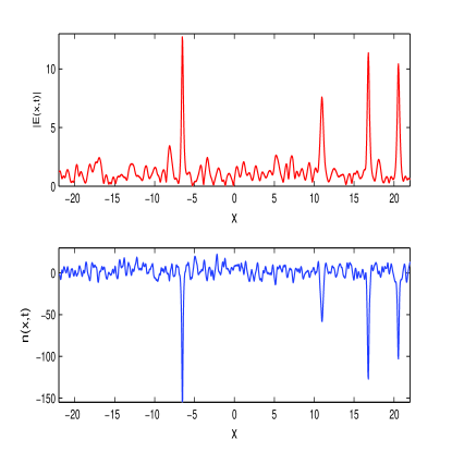
Figure 1: (Color online) The profiles of the wave electric field $E(x,t)$ (upper panel) and the associated density fluctuation $n(x,t)$ (lower panel) with respect to the space $x$ after time $t=200$ in the numerical simulation of the QZEs for $k=0.14$, $H=0$ and $E_{0}=2$.

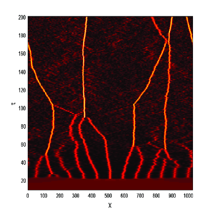
Figure 2: (Color online) Space-time contour plots of  $\left|E(x,t)\right|=$constant corresponding to the evolution as in Fig. 1. This shows that pattern selection leads to many solitary patterns which due to QIAW emission collide and get fused into few incoherent patterns after a long time. The STC state emerges.

Note that as above the MI sets in for wave numbers satisfying $0<k<k_{c},$ where $k_{c}$ is a real root of the cubic $H^{2}k^{3}+k-\sqrt{2}E_{0}=0,$ and $k=k_{c}$ defines the curve along which pitchfork bifurcation takes place. Moreover, the dynamics is subsonic in the regime $k_{c}/2<k<k_{c}$ where the MI growth rate is small. As $k$ is lowered from $k_{c}/2,$ many unstable modes with higher harmonic modes will be excited.  Again, the master mode can, in principle, result in the excitation of $N-1$ unstable harmonic modes where $N=[\bar{k}^{-1}]$ with $\bar{k}=k/\sqrt{2}E_{0}.$ There may also exist many solitary patterns with spatially modulated length $l_{m}=L/m,$ where $m=1$ is for master mode ($l_{1}=L=2\pi/k$) and $m=2,3,....,M$ are for the unstable harmonic modes. As a result, the envelope $E$ can be expressed as:

$$E(x,t)={\displaystyle\sum\limits_{m=1}^{M}}E_{m}(t)\exp(im\bar{k}x)+{\displaystyle\sum\limits_{m=M+1}^{\infty}}E_{m}(t)\exp(im\bar{k}x),$$ (5)

in which the first term on the right-side of Eq. (5) comes from the master mode and unstable harmonic modes with $M<N-1$ being due to pattern selection, whereas the second term is due to the nonlinear interaction among the patterns formed.

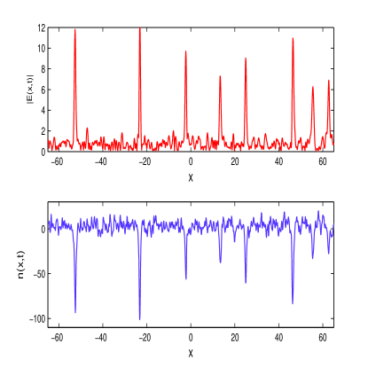
Figure 3: (Color online) The same as in Fig. 1, but for $H=0.2$, $k=0.048$ and other parameters remain the same as in Fig. 1.

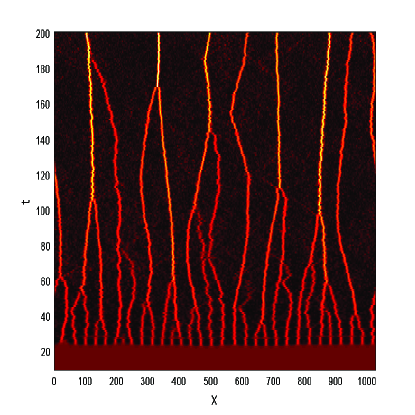
Figure 4: (Color online) Contours of  $\left|E(x,t)\right|=$constant with respect to space and time corresponding to the evolution as in Fig. 3. This shows that pattern selection leads to many more solitary patterns than the classical case (Fig. 2) which due to QIAW emission collide and get fused into few incoherent patterns after a long time. The collision is random and not confined between two patterns. Few stable modes are also excited. The system energy is then redistributed to new incoherent patterns and few stable modes with small length scales. The system is in the state of STC.

The profiles of the electric field and the density fluctuation at the end of simulation are shown in Fig.1 for $k=0.14$ and $H=0$. We observe an excited electric field of the order $|E|\sim 12$ highly correlated with density depletion $n\sim-152$ or $n/n_{0}\sim-0.33.$ From Fig. 2, we find that many solitary patterns are formed from the master mode and unstable harmonic modes by means of pattern selection. Two solitary patterns initially peaked in $100<x<200$ collide to form a new mode which again collides with the master pattern peaked at $x\sim 50$ and fuses into a new strong mode. After few more other collisions and fusions, there remain only four distorted patterns. The system is then said to emerge the STC state. When $k$ is further lowered many solitary trains are excited and saturated. As soon as the collisions and fusions among the solitary patterns take place and the new incoherent trains are formed under strong QIAW emission, these incoherent patterns then collide with some others repeatedly and finally there remain few incoherent patterns in stochastic motion with the greater part of the system energy. Meanwhile many stronger modes are also excited to share the energy. These are shown in Figs. 3, 4 and Figs. 5, 6 for different values of $H$: $H=0.2$ and $0.5$ respectively. We observe that though the number of remaining modes are the same for both the cases, however, many more (compared to Fig. 6) solitary patterns are seen to form initially (Fig. 4) which later participate into the collisions and fusions under QIAW emission. Moreover, the new incoherent patterns formed with the lapse of long time are more stronger as in Fig. 6 than those in Fig. 4. Furthermore, for higher values of $H$ (Fig. 6) the collisions and fusions take place at an earlier time than the case of lower $H$ (Fig.4). Thus, a certain amount of energy which was initially distributed among many solitary waves, will now be transferred to a few incoherent patterns as well as to some stable higher harmonic modes with short wave lengths. So, if initially there form many solitary pattern trains due to MI with different modulational lengths, collision and fusion among most them can lead to the STC state. There must exist a critical wavelength or wave number $k,$ at which the transition from temporal chaos to STC takes place. This value, in the quantum case ($H\neq 0$) is quite different from the classical one ($H=0$). For detail investigations readers are referred to works, e.g., in Refs. Spatiotemporal1 ; Spatiotemporal2 .

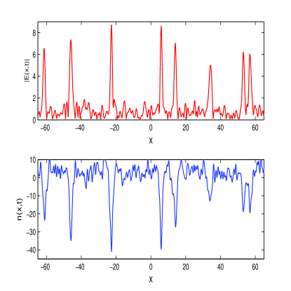
Figure 5: (Color online) The same as in Fig. 3, but for different $H=0.5$. Other parameters remain the same as in Fig. 3.

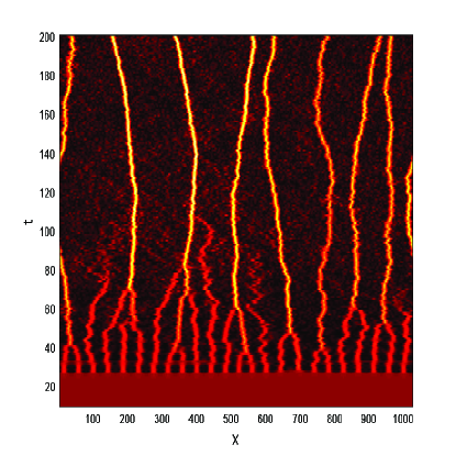
Figure 6: (Color online) Contours of  $\left|E(x,t)\right|=$constant with respect to space and time corresponding to the evolution as in Fig. 5. Here the pattern selection leads to many solitary patterns, but less than that in Fig. 4. Though, the collision is random and not confined between two patterns, but they fuse into new incoherent patterns in a shorter time than the case of $H=0.2$ (Fig. 4) due to strong QIAW emission. The system is also in the STC state.

III Conclusion

We have performed a simulation study of the QZEs to show that many coherent solitary patterns can be excited and saturated through the MI of unstable harmonic modes by a modulation wave number of QLWs. It is observed that there exist critical values of $k$ for which the motion of the coherent solitary patterns is in the state of TC or in STC. The transition from TC to STC occurs when $k\lesssim 0.14$ for $H=0$ or, for $k\lesssim 0.048\$when $H\gtrsim 0.2.$ It is shown that the dispersion due to quantum tunneling induces strong QIAW emission leading to collision and fusion among the patterns to occur at an earlier time than the classical case. The Collision and fusion among some trains take place and the new incoherent pattern trains are formed accompanying strong QIAW emission due to quantum effects. The STC state is then said to emerge. As a result, the system energy in the STC state is spatially redistributed in the process of pattern collision, fusion and distortion, which may switch on the onset of Langmuir turbulence in quantum plasmas.

IV Acknowledgments

This work was prepared in honor of Professor P. K. Shukla’s 60th birthday.  A. P. M gratefully acknowledges support from the Kempe Foundations, Sweden.

References

- (1) L. G. Garcia, F. Haas, J. Goedert, and L. P. L. Oliveira, Phys. Plasmas 12, 012302 (2005).
- (2) V. E. Zakharov, Sov. Phys. JETP 35, 908 (1972).
- (3) F. Haas, Phys. Plasmas 14, 042309 (2007).
- (4) X. Y. Tang and P. K. Shukla, Phys. Scr. 76, 665 (2007).
- (5) M. A. Abdou and E. M. Abulwafa, Z. Naturforsch., A: Phys. Sci. 63a, 646 (2008); S. A. El-Waki and M. A. Abdou, Nonlinear Anal. Theory, Methods Appl. 68, 235 (2008).
- (6) A. P. Misra, D. Ghosh, and A. R. Chowdhury, Phys. Lett. A 372, 1469 (2008); A. P. Misra, S. Banerjee, F. Haas, P. K. Shukla, and L. P. G. Assis, Phys. Plasmas 17, 032307 (2010).
- (7) A. P. Misra and P. K. Shukla, Phys. Rev. E 79, 056401 (2009).
- (8) M. Marklund, Phys. Plasmas 12, 082110 (2005).
- (9) F. Haas and P. K. Shukla, Phys. Rev. E 79, 066402 (2009).
- (10) G. Simpson, C. Sulem, and P. L. Sulem, Phys. Rev. E 80, 056405 (2009).
- (11) F. B. Rizzato, G. I. de Oliveira, and R. Erichsen, Phys. Rev. E 57, 2776 (1998).
- (12) X. T. He, C. Y. Zheng, and S. P. Zhu, Phys. Rev. E 66, 037201 (2002).
- (13) S. Banerjee, A. P. Misra, P. K. Shukla, and L. Rondoni, Phys. Rev. E 81, 046405 (2010).