Search for light-speed anisotropies using Compton scattering of high-energy electrons

Abstract

Based on the high sensitivity of Compton scattering off ultra relativistic electrons, the possibility of anisotropies in the speed of light is investigated. The result discussed in this contribution is based on the $\gamma$-ray beam of the ESRF’s GRAAL facility (Grenoble, France) and the search for sidereal variations in the energy of the Compton-edge photons. The absence of oscillations yields the two-sided limit of $1.6\times 10^{-14}$ at $95\,\%$ confidence level on a combination of photon and electron coefficients of the minimal Standard Model Extension (mSME). This new constraint provides an improvement over previous bounds by one order of magnitude.

Experimental searches for anisotropies in $c$ and, more generally, for Lorentz violating (LV) processes are currently motivated by theoretical studies in the context of quantum gravity. Recent approaches to Planck-scale physics can indeed accommodate minuscule violations of Lorentz symmetry [1].

The present result is based on a laboratory experiment using only photons and electrons in an environment where gravity is negligible. Lorentz violation can then be described by the single-flavor QED limit of the flat-spacetime mSME [2, 5]. In this framework, photons have a modified dispersion relation:

$$\omega=(1-\vec{\kappa}\cdot\hat{\lambda})\,\lambda+{\mathcal{O}}(\kappa^{2})\;.$$ (1)

Here, $\lambda^{\mu}=(\omega,\lambda\hat{\lambda})$ denotes the photon 4-momentum and $\hat{\lambda}$ is a unit 3-vector. The space-time constant mSME $\vec{\kappa}$ vector specifies a preferred direction in the Universe which violates Lorentz symmetry, and can be interpreted as generating a direction-dependent refractive index of the vacuum $n(\hat{\lambda})\simeq 1+\vec{\kappa}\cdot\hat{\lambda}$.

The basic experimental idea is that in a terrestrial laboratory the photon 3-momentum in a Compton-scattering process changes direction due to the Earth’s rotation. The photons are thus affected by the anisotropies in Eq. (1) leading to sidereal effects in the kinematics of the process.

The experimental set-up at GRAAL involves counter-propagating incoming electrons and photons with 3-momenta $\vec{p}=p\,\hat{p}$ and $\vec{\lambda}=-\lambda\,\hat{p}$, respectively. The conventional Compton edge (CE) then occurs for outgoing photons that are backscattered at $180^{\circ}$, so that the kinematics is essentially one dimensional along the beam direction $\hat{p}$. Energy conservation for this process reads

$$E(p)+(1+\vec{\kappa}\cdot\hat{p})\,\lambda=E(p-\lambda-\lambda^{\prime})+(1-\vec{\kappa}\cdot\hat{p})\,\lambda^{\prime}\;,$$ (2)

where $\vec{\lambda}^{\prime}=\lambda^{\prime}\,\hat{p}$ is the 3-momentum of the CE photon, and 3-momentum conservation has been implemented. At leading order, the physical solution of Eq. (2) is

$$\lambda^{\prime}\simeq\lambda_{\rm CE}\left[\,1+\frac{2\,\gamma^{2}}{(1+4\,\gamma\,\lambda\,/\,m)^{2}}\,\vec{\kappa}\cdot\hat{p}\,\right]\,.$$ (3)

Here, $\lambda_{\rm CE}=\frac{4\,\gamma^{2}\,\lambda}{1+4\,\gamma\,\lambda\,/\,m}$ denotes the conventional value of the CE energy. Given the actual experimental data of $m=511\,$keV, $p=6030\,$MeV, and $\lambda=3.5\,$eV, yields $\gamma\simeq p/m=11800$ and $\lambda_{\rm CE}=1473\,$MeV. The numerical value of the factor in front of $\vec{\kappa}\cdot\hat{p}$ is about $1.6\times 10^{8}$. It is this large amplification factor (essentially given by $\gamma^{2}$) that yields the exceptional sensitivity of the CE to $\tilde{\kappa}_{o+}$.

Expressed in the Sun-centered inertial frame $(X,Y,Z)$ [4] and taking into account GRAAL’s latitude and beam direction, eq. (3) becomes

$$\lambda^{\prime}\simeq\tilde{\lambda}_{\rm CE}+0.91\,\frac{2\,\gamma^{2}\,\lambda_{\rm CE}}{(1+4\,\gamma\,\lambda\,/\,m)^{2}}\sqrt{\kappa_{X}^{2}+\kappa_{Y}^{2}}\,\sin\Omega t\,.$$ (4)

Incoming photons overlap with the ESRF beam over a $6.5\,$m long straight section. Due to their energy loss, scattered electrons are extracted from the main beam in the magnetic dipole following the straight section. Their position can then be accurately measured in the so-called tagging system located $50\,$cm after the exit of the dipole. This system is composed of a position-sensitive Si $\mu$-strip detector (128 strips of $300\,$$\mu$m pitch, $500\,$$\mu$m thick) associated to a set of fast plastic scintillators. A typical Si $\mu$-strip count spectrum near the CE is shown in Fig. 1 for the multiline UV mode ($364$, $351$, $333\,$nm) of the laser used in this measurement. The fitting function, also plotted, is based on the sum of 3 error functions plus background and includes 6 free parameters. The CE position (location of the central line), $x_{\rm CE}$, can be measured with an excellent resolution of $\sim 3\,\mu$m.

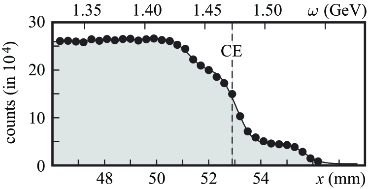
Figure 1: Si $\mu$-strip count spectrum near the CE and the fitting function (see text) vs. position $x$ and photon energy $\omega$. The three edges corresponding to the lines $364$, $351$, and $333\,$nm are clearly visible. The CE position $x_{\rm CE}$ is the location of the central line and is measured with a typical accuracy of $3\,$$\mu$m.

A sample of the time series of the CE positions relative to the ESRF beam covering $24\,$h is displayed in Fig. 2c, along with the tagging-box temperature (Fig. 2b) and the ESRF beam intensity (Fig. 2a). The sharp steps present in Fig. 2a correspond to the twice-a-day refills of the ESRF ring. The similarity of the temperature and CE spectra combined with their correlation with the ESRF beam intensity led us to interpret the continuous and slow drift of the CE positions as a result of the tagging-box dilation induced by the x-ray heat load.

To get rid of this trivial time dependence, raw data have been fitted with the sum of two exponential whose time constants have been extracted from the time evolution of the temperature data. The corrected and final spectrum is obtained by subtraction of the fitted function from the raw data, (Fig. 2d).

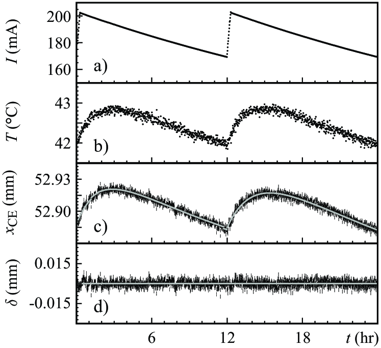
Figure 2: Time evolution over a day of a) ESRF beam intensity; b) tagging-box temperature; c) CE position and fitted curve; d) $\delta=x_{\rm CE}-x_{\rm fit}$. The error bars on position measurements are directly given by the CE fit.

The usual equation for the deflection of charges in a magnetic field together with momentum conservation in Compton scattering determines the relation between the CE variations $\frac{\Delta x_{\rm CE}}{x_{\rm CE}}$ and a hypothetical CE photon 3-momentum oscillation $\frac{\Delta\lambda^{\prime}}{\lambda^{\prime}}$:

$$\frac{\Delta x_{\rm CE}}{x_{\rm CE}}=\frac{p}{p-\lambda_{\rm CE}}\frac{\Delta\lambda^{\prime}}{\lambda^{\prime}}\,.$$ (5)

To search for a modulation, 14765 data points collected in about 1 week of data taking have been folded modulo a sidereal day (Fig. 3). The error bars are purely statistical and the histogram is in agreement with a null signal ($\chi^{2}=1.04$). To look for a harmonic oscillation ($A\sin(\Omega t+\phi)$), we have performed a statistical analysis based on the Bayesian approach. The resulting upper bound is $A<2.5\times 10^{-6}$ at $95\%$ CL.

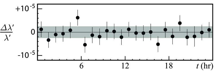
Figure 3: Full set of data folded modulo a sidereal day (24 bins). The error bars are purely statistical and agree with the dispersion of the data points ($\chi^{2}=1.04$ for the unbinned histogram). The shaded area corresponds to the region of non-excluded signal amplitudes.

We next consider effects that could conceal an actual sidereal signal. Besides a direct oscillation of the orbit, the two quantities that may affect the result are the dipole magnetic field and the momentum of the ESRF beam $p$. All these parameters are linked to the machine operation, and their stability follows directly from the accelerator performance. A detailed analysis of the ESRF database allows us to conclude that a sidereal oscillation of any of these parameters cannot exceed a few parts in $10^{7}$ and is negligible.

We can now conclude that our upper bound on a hypothetical sidereal oscillation of the CE energy is:

$$\Delta\lambda^{\prime}/\lambda^{\prime}<2.5\times 10^{-6}\quad(95\,\%\;{\rm CL})\,,$$ (6)

yielding the competitive limit $\sqrt{\kappa_{X}^{2}+\kappa_{Y}^{2}}<1.6\times 10^{-14}$ ($95\,\%$ CL) with Eq. (4) [6]. This limit improves previous bounds by a factor of ten and represents the first test of Special Relativity via a non-threshold kinematics effect in a particle collision [7].

References

- [1] See, e.g., V.A. Kostelecký and S. Samuel, Phys. Rev. D 39, 683 (1989); J. Alfaro, H.A. Morales-Técotl, and L.F. Urrutia, Phys. Rev. Lett. 84, 2318 (2000); S.M. Carroll et al., Phys. Rev. Lett. 87, 141601 (2001); J.D. Bjorken, Phys. Rev. D 67, 043508 (2003); V.A. Kostelecký et al., Phys. Rev. D 68, 123511 (2003); F.R. Klinkhamer and C. Rupp, Phys. Rev. D 70, 045020 (2004); N. Arkani-Hamed et al., JHEP 0507, 029 (2005).
- [2] D. Colladay and V.A. Kostelecký, Phys. Rev. D 55, 6760 (1997); Phys. Rev. D 58, 116002 (1998); V.A. Kostelecký and R. Lehnert, Phys. Rev. D 63, 065008 (2001); V.A. Kostelecký, Phys. Rev. D 69, 105009 (2004).
- [3] For recent reviews see, e.g., V.A. Kostelecký, ed., CPT and Lorentz Symmetry I-IV, World Scientific, Singapore, 1999-2008; R. Bluhm, Lect. Notes Phys. 702, 191 (2006); D.M. Mattingly, Living Rev. Rel. 8, 5 (2005).
- [4] V.A. Kostelecký and N. Russell, arXiv:0801.0287.
- [5] M.A. Hohensee et al., Phys. Rev. Lett. 102, 170402 (2009); Phys. Rev. D 80, 036010 (2009); B.D. Altschul, Phys. Rev. D 80, 091901 (2009).
- [6] J.-P. Bocquet et al., Phys. Rev. Lett. 104, 241601 (2010);
- [7] R. Lehnert, Phys. Rev. D 68, 085003 (2003).