Modelling the light variability of the Ap star $\varepsilon$ Ursae Majoris

Abstract

Aims. We simulate the light variability of the Ap star $ε$ UMa using the observed surface distributions of Fe, Cr, Ca, Mn, Mg, Sr, and Ti obtained with the help of the Doppler imaging technique.

Methods. Using all photometric data available, we specified light variations of $\varepsilon$ UMa modulated by its rotation from far UV to IR. We employed the LLmodels stellar model atmosphere code to predict the light variability in different photometric systems.

Results. The rotational period of $\varepsilon$ UMa is refined to $5\aas@@fstack{d}088631(18)$. It is shown that the observed light variability can be explained as a result of the redistribution of radiative flux from the UV spectral region to the visual caused by the inhomogeneous surface distribution of chemical elements. Among seven mapped elements, only Fe and Cr contribute significantly to the amplitude of the observed light variability. In general, we find very good agreement between theory and observations. We confirm the important role of Fe and Cr in determining the magnitude of the well-known depression around $5200$ Å by analyzing the peculiar $a$-parameter. Finally, we show that the abundance spots of considered elements cannot explain the observed variabilities in near UV and $\beta$ index, which probably have other causes.

Conclusions. The inhomogeneous surface distribution of chemical elements can explain most of the observed light variability of the A-type CP star $\varepsilon$ UMa.

1 Introduction

Chemically peculiar (CP) stars are main-sequence A- and B-type stars that have a number of characteristic photometric and spectroscopic anomalies. Slow rotation (and, consequently, weak meridional currents), globally structured magnetic fields, and weak convection allow a build up of the prominent abundance anomalies and inhomogeneities as a result of particle diffusion driven by the radiation field (first proposed by Michaud, 1970). These inhomogeneities are frequently seen as abundance spots on stellar surfaces (see, for example, Khokhlova et al., 2000; Kochukhov et al., 2004; Lehmann et al., 2007), and as clouds of chemical elements concentrated at different heights in stellar atmospheres (Ryabchikova et al., 2002, 2008; Kochukhov et al., 2006; Shulyak et al., 2009, and references therein).

Among the defining characteristics of CP stars, their light variability in different photometric systems still awaits quantitative explanation. That this variability is seen in independent systems, simultaneously in narrow- and broad-band bands, and in anti-phase in far-UV and optical spectral regions suggests that the global flux redistribution caused by the phase-dependent absorption is the probable cause of the observed phenomena (Molnar, 1973, 1975). If so, there may be a point (or points or even regions, see Mikulášek et al., 2007b ) in the spectra where the flux remains almost unchanged, and vary more or less in anti-phase on both sides from it. This region, called a “null wavelength region”, has been noted and confirmed by a number of studies (see, for example, Leckrone, 1974; Molnar, 1973; Jamar, 1977; Sokolov, 2000, 2006). However, that the truly “null wavelength region” in stars with more complex light curves may not exist (Sokolov, 2006, 2010). The connection between the abundance spots and flux redistribution has emerged as a natural explanation of the rotationally modulated light curves of CP stars, but the details of this relation still have to be determined on a solid theoretical basis.

With the appearance of detailed abundance Doppler images (DI) of the stellar surfaces (e.g., Lüftinger et al., 2003; Kochukhov et al., 2004; Lehmann et al., 2007) and advanced computers it became possible to numerically explore the role of uneven distributions of chemical elements as a source of the light variability. First, Krtička et al., (2007) succeeded in reproducing the light variability of a hot ($T_{\rm eff}=22000$ K) Bp star HD 37776 based on the DI maps of He and Si derived by Khokhlova et al., (2000). Later, Krtička et al., (2009) successfully fitted the light curves of a cooler ($T_{\rm eff}=14500$ K) Bp star HR 7224 using Fe and Si maps presented by Lehmann et al., (2007). The main result of both studies is a very good, parameter-free theoretical explanation of both the shapes and amplitudes of the observed light curves. The authors thus proved, on the one side, that an inhomogeneous surface distribution of chemical elements accounts for most of the light variability in these stars, and, on the other side, they independently confirmed the results of DI mapping. In spite of significant progress in this direction, the role of abundance spots (and individual elements) in CP stars cooler than B-type remains unknown.

In this paper, we continue to present results of the light-curve modelling of CP stars, concentrating on the brightest A-type CP star $\varepsilon$ UMa (HD 112185, HR 4905). This star has been studied extensively in the past and many good photometric observations are available, including the data obtained by space photometry experiments. The surface distributions of seven elements (Ca, Cr, Fe, Mg, Mn, Sr, Ti) were derived via the DI technique by Lüftinger et al., (2003), providing the necessary basis for theoretical modelling of the photometric variability.

2 Observations

The CP star $\varepsilon$ UMa is a well-known spectral, magnetic, and photometric variable star. The ${Ca\textsc{ii}}$ K line and profuse lines of ${Cr\textsc{ii}}$ vary oppositely in strength with a period of $5\aas@@fstack{d}0877$ (Guthnick, 1931, 1934; Struve & Hiltner, 1943; Swensson, 1944; Deutsch, 1947). Photometric variations are observed to have the same period, but to have double waves (Provin, 1953; Musielok et al., 1980; Pyper & Adelman, 1985, etc.) with the maximum light occurring at ${Ca\textsc{ii}}$ minimum chosen to be the phase 0.00. Far ultraviolet OAO-2 spectrometer observations of $\varepsilon$ UMa indicate strong light variations in the anti-phase with optical ones (Molnar, 1975; Mallama & Molnar, 1977).

Spectropolarimetry of $\varepsilon$ UMa has detected its very weak variable magnetic field whose maximum coincides with the optical light maximum (Borra & Lanstreet 1980; Bohlender & Landstreet, 1990; Donati & Semel, 1990; Wade et al., 2000).

Until now, almost all papers dealing with variations in the light of $\varepsilon$ UMa have used the Guthnick, (1931) ephemeris

$$\mathit{HJD}({Ca\textsc{ii}}\ \mathrm{min.\,int.})=2\,426\,437.01+5\aas@@fstack{d}0887\times E,$$ (1)

where $E$ is the epoch.

In this paper, we use light curves observed in different photometric systems. Strömgrem $\mathit{uvby}$ measurements were taken from Pyper & Adelman, (1985), and extended by 10-color medium-band Shemakha photometry with filters similar to standard $\mathit{uvby}$ filters (Musielok et al., 1980). $B$ and $V$ observations close to the Johnson standard were performed by Provin, (1953). Unfortunately, no reliable data has been obtained in the broad-band $U$ filter, the available $\mathit{UBV}$ observations of Srivastava, (1989) been ususable due to their excessive scatter. The same concerns available data in the $B_{\rm T}$ and $V_{\rm T}$ passbands from Tycho catalog, while Hipparcos $H_{\rm P}$ photometric measurements (ESA, 1997) are well calibrated and were used here in the light curve modelling.

We also used photometric data derived by Molnar, (1975) and Mallama & Molnar, (1977) using spectrometry of $\varepsilon$ UMa performed by the ultraviolet satellite OAO-2 (more about the project is given in Code et al., 1970). We also attempted to use spectroscopic observations obtained by the International Ultraviolet Explorer (IUE) and Copernicus space missions available via the Multimission Archive at STScl. Finally, we used a dataset of photometric observations carried out by the Wide Field Infrared Explorer (WIRE) obtained during June-July 2000, although we had to rejected several parts strongly affected by instrumental effects and instabilities (see Retter et al., 2004, for details).

3 Methods

3.1 Model atmospheres

To perform the model atmosphere calculations, we used the most recent version of the LLmodels  (Shulyak et al., 2004) stellar model atmosphere code. For all calculations, local thermodynamical equilibrium (LTE) and plane-parallel geometry were assumed. The VALD database (Piskunov et al., 1995; Kupka et al., 1999) was used as a main source of the atomic line data for computation of the line absorption coefficient. The VALD compilation contains information about $66\times 10^{6}$ atomic transitions. Most of them come from the latest theoretical calculations performed by R. Kurucz.

The global magnetic field of the star is very weak (of polar intensity on the order of a few hundred Gauss (Donati & Semel, 1990; Bohlender & Landstreet, 1990)), which allows us to ignore its possible effect on the variability of the outgoing flux.

3.2 Calculation of the light curve

In previous attempts to simulate the light curves of HD 37776 (Krtička et al., 2007) and HR 7224 (Krtička et al., 2009), the following approach has been taken:

1. The construction of a grid of model atmospheres for a number of abundances combinations that cover the parameter space provided by DI maps.

2. Interpolation of specific intensities (or fluxes) from the grid onto a combination of abundances for all meshes visible at a given phase of rotation. The resulting flux is then obtained by surface integration of specific intensities (or fluxes with assumed limb-darkening law).

This procedure is applied to every rotational phase and wavelength interval occupied by a given photometric filter. Although simple, this approach becomes challenging when modelling the light curves of $\varepsilon$ UMa. Indeed, in both cases of HD 37776 and HR 7224, only two elements were mapped (He and Si for the former; Fe and Si for the latter). To produce a smooth light curve, it was enough to compute a grid containing tens of models with different sets of abundances. Obviously, with the increasing number of mapped elements, the number of models needed to perform abundance interpolation can become comparable or even larger than the number of surface elements originally used in DI calculations.

Seven mapped elements of $\varepsilon$ UMa would require time-consuming computations. We instead use a slightly different approach. To reduce computational expenses, we decrease the resolution of DI maps by interpolating them from the original grid of longitudes and latitudes onto a more sparse one. Then, for every pair of new latitude and longitude, we compute a model atmosphere with individual abundances that represent a given surface mesh. Next, for every model (i.e. surface mesh), we compute the light curves in a particular photometric filter with the help of modified computer codes taken from Kurucz, (1993) and extended by Hipparcos photometry with passbands from Bessel, (2000). The expected magnitude at a given phase $c_{\rm phase}$ is obtained by surface integration of individual fluxes $F_{i}$ from all visible meshes

$$c_{\rm phase}=-2.5\log\left[\displaystyle\frac{1}{U}\displaystyle\int\limits_{\mathrm{\scriptstyle visible\;surface}}F_{i}\cos\theta_{i}u(\theta_{i})dS\right],$$ (2)

where $\theta$ is the angle between the normal to the surface element and the line of sight, $u(\theta)$ describes the limb darkening for a given filter, which we assume to be a quadratic law, i.e.,

$$u(\theta)=1-a(1-\cos\theta)-b(1-\cos\theta)^{2},$$ (3)

and $U$ is given by

$$U=\displaystyle\int\limits_{\mathrm{\scriptstyle visible\;surface}}u(\theta_{i})\cos\theta_{i}dS.$$ (4)

We adopted the same limb darkening coefficients regardless of the true surface elements. In particular, the quadratic coefficients $a$ and $b$ in each color were taken from the tables of Claret, (2000) for the solar abundance model. For the Hipparcos $H_{\rm P}$ filter, these coefficients were taken to be the average between the Johnson $B$ and $V$ filters. Since there is no definite filter curve for the WIRE star tracker, limb darkening coefficients for Johnson $V$ filter were used instead (H. Bruntt, private communication). Because of this uncertainty, the WIRE photometry is presented in this paper mainly for illustrative purposes.

The original resolution of DI maps of $\varepsilon$ UMa is $33$ latitude and $68$ longitude points equidistantly spaced between $[0,180]$ and $[0,360]$ spherical angles. To reduce the number of calculations, we decreased the resolution of maps to $15$ and $30$ latitude and longitude points, respectively. As proven by numerical tests, this decrease in resolution provides abundance maps smooth enough for an accurate representation of the light curves: we found no visible differences in light curves when computing all $2244$ models at the original resolution, and $450$ models from the reduced grid (see Sect. discussion for more details). Thus, in the remaining light curve modelling presented in this work we always used a lower number of $450$ surface elements than the $2244$ original.

Table 1 summarizes the basic stellar parameters adopted in the present study taken from Lüftinger et al., (2003). The abundances are given relative to the total number ot atoms, i.e. $\varepsilon_{\rm el}=log(N_{\rm el}/N_{\rm total})$.

Table 1: Stellar parameters of $\varepsilon$ UMa.

Effective temperature $T_{\rm eff}$	$9000$ K
Surface gravity $\log g$ (cgs)	$3.6$
Inclination angle $i$	$45^{\circ}$
Abundance ranges from DI maps
Ca	$[-6.149,-4.628]$
Cr	$[-8.270,-1.559]$
Fe	$[-6.529,-2.582]$
Mg	$[-5.686,-3.285]$
Mn	$[-6.281,-4.890]$
Sr	$[-11.515,-3.967]$
Ti	$[-8.478,-6.561]$

4 Results

4.1 Improved ephemeris

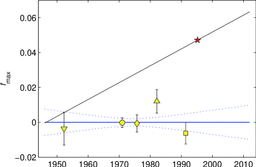
Figure 1: The dependence of the primary maximum phases derived from Eq. 7 on time. $\nabla$ – BV photometry (Provin, 1953), full circle – UV photometry from OAO-2 satellite (Molnar, 1975), $\Diamond$ – 10-color medium-band photometry (Musielok & Madej, 1988), $\Box$ – Hipparcos photometry (ESA, 1997), $\triangle$ ubvy photometry of Pyper & Adelman, (1985), the oblique line represents the Guthnick’s ephemeris from Eq. (1), and the star on it the phase position to which are referred the spectroscopic maps we used.

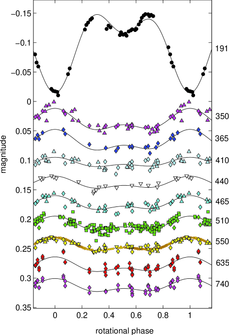
Figure 2: Observed light curves constructed from original data in several passdands, whose effective wavelengths in nm are given on the right. For clarity, individual LCs are shifted in their magnitudes. Full circles – UV photometry from OAO-2 satellite (Molnar, 1975), $\Diamond$ – 10-color medium-band photometry (Musielok et al., 1980), $\triangle$ ubvy photometry of Pyper & Adelman, (1985), $\nabla\ -\ \mathit{BV}$ (Provin, 1953), $\Box\ -$ Hipparcos photometry (ESA, 1997), and small full circles relate to broad-band photometry of WIRE (Retter et al., 2004) - each point is the median of 1600 individual time-consecutive measurements.

Table 2: Maximum phases according to individual sources of photometric data. $\Delta\varphi$ is the difference between new phases and phases evaluated according former ephemeris, see Eq. (8).

Year	max. phase	$\Delta\varphi$	$N$	source
1952.3	-0.004(10)	0.006	36	Provin, (1953)
1971.0	-0.000(3)	0.024	38	Molnar, (1975)
1975.7	-0.001(5)	0.028	179	Musielok et al., (1980)
1982.1	0.012(7)	0.035	39	Pyper & Adelman, (1985)
1991.4	-0.006(6)	0.044	175	ESA, (1997)
1995.2		0.047		Lüftinger et al., (2003)

Observational data used in the following analyzes of rotationally modulated variations of $\varepsilon$ UMa were obtained in the past 70 years during which the star has revolved more than five thousand times. Although we do not know the true uncertainty in the determination of the canonical rotational period $P=5\aas@@fstack{d}0887$ published by Guthnick, (1931) it can hardly be better than $\pm 0\aas@@fstack{d}0001$! This uncertainty manifests itself in the uncertainty of $0\aas@@fstack{p}1$ in the rotational phase determination, which is for reliable studies unacceptable.

This compelled us to improve the $\varepsilon$ UMa rotational period. For this purpose, we used all available reliable photometric data, especially the 36 $BV$ measurements of Provin, (1953), 38 synthetic magnitudes derived from spectrometric data in 191 nm by Molnar, (1973), 179 individual observations in the ten-color Shemakha medium-band system taken by Musielok et al., (1980), 80 Strömgreen $\mathit{uvby}$ measurements obtained by Pyper & Adelman, (1985), andthe 314 $B_{\mathrm{T}}V_{\mathrm{T}}$, and 122 $H_{\rm P}$ measurements derived from data of the Hipparcos satellite (ESA, 1997). Thus, we had 769 individual measurements covering the period of 1952–1993 (see Table 2); unfortunately measurements from the present time were absent. Measurements taken in various narrow- and broad-band filters were divided into 10 groups according to their effective wavelengths - see Table 3.

We also used a very extensive data-set of WIRE photometry (Retter et al., 2004), which was unfortunately unreliable in several ways:

1. We have been unable to interconnect the timing of its measurements with standard HJD timing.

2. Because of their large scatter and instabilities, we omitted the first part of measurements and then one day of measurements.

3. We found that consecutive measurements are not independent. We therefore aggregated WIRE measurements into groups of about 1600 members. Altogether we used 195 normal points with standard uncertainty of 0.55 mmag.

4. We identified significant trends in the observations, but which could be represented well by cubic polynomials and removed.

The double-waved light curves are more or less similar (see Fig. 2), differing only in their effective amplitudes $A_{c}$ (for a definition, see Mikulášek et al., 2007a ), where the subscript $c$ denotes the photometric passband. Light-curve magnitudes can then be expressed as

$$m_{cj}(t)\simeq\overline{m}_{cj}+\textstyle{\frac{1}{2}}\,A_{c}F(\vartheta),$$ (5)

where $m_{cj}(t)$ is the magnitude in color $c$ observed by the $j$-th observer, $\overline{m}_{cj}$ is the mean magnitude, which can be variable over the long term. This was the case for WIRE measurements, where we had to assume a cubic trend.

Table 3: Dependence of the effective amplitude of light variations on wavelength. $N$ denotes the number of measurements.

$\lambda_{\mathrm{eff}}$ [nm]	$A_{\mathrm{eff}}$ [mag]	$N$	effective filter
191	0.1232(25)	38	Molnar
350	-0.0336(22)	38	$u,\,U_{10}$
360	-0.0325(33)	18	$P_{10}$
410	-0.0147(27)	39	$v,\,X_{10}$
440	-0.0190(22)	175	$B,\,B_{\rm{T}}$
465	-0.0218(18)	38	$b,\,Y_{10}$
510	-0.0220(15)	140	$H_{p},\,Z_{10}$
550	-0.0209(01)	407	$V,\,y,\,V_{\rm{T}},\,V_{10},\,\mathit{WIRE}$
635	-0.0230(33)	37	$\mathit{HR}_{10},\,S_{10}$
740	-0.0205(28)	34	$\mathit{MR}_{10},\,\mathit{DR}_{10}$

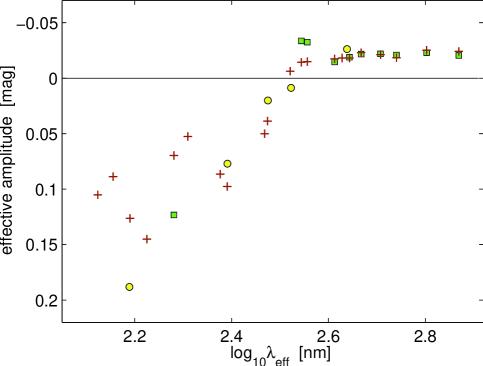
Figure 3: Effective amplitudes of observed light curves taken in various effective wavelengths. Squares correspond to the amplitudes of LCs taken in individual photometric filters, full circles are values adopted from Mallama & Molnar, (1977), and crosses are effective amplitudes of LCs modelled in this work.

Function $F(\vartheta)$ is the simplest normalised periodic function that represents the observed photometric variations of $\varepsilon$ UMa in detail. The phase of maximum brightness is defined to be 0.00, and the effective amplitude is defined to be 1.0. The function, being the sum of three terms, is described by two dimensionless parameters $\beta_{1}$ and $\beta_{2}$, where $\beta_{1}$ quantifies the difference in heights of the primary and the secondary maxima and $\beta_{2}$ expresses any asymmetry in the light curve

$$F(\vartheta,\,\beta_{1},\,\beta_{2})=\sqrt{1\!-\!\beta_{1}^{2}\!-\!\beta_{2}^{2}}\ \cos(2\,\pi\,\vartheta)+\,\beta_{1}\cos(4\,\pi\,\vartheta)+$$

$$\beta_{2}\left[\textstyle{\frac{2}{\sqrt{5}}}\,\sin(2\,\pi\,\vartheta)-\textstyle{\frac{1}{\sqrt{5}}}\sin(4\,\pi\,\vartheta)\right],$$ (6)

where $\vartheta$ is the phase function. The O-C diagram (see Fig. 1 and Table 2) indicates that the function is linear; thus, we assumed it to have the form

$$\vartheta=\left(t-M_{0}\right)/P,\quad\mathit{HJD}(\mathrm{max\,I})=M_{0}+P\times E,$$ (7)

where $P$ is the period of the linear fit and $M_{0}$ is the HJD time of the primary maximum nearest the weighted centre of all observations except WIRE ones. The time of basic primary maximum in WIRE timing is then $M_{0\rm{W}}$. All 39 model parameters were computed simultaneously by a weighted non-linear LSM regression applied to the complete observational material.

We found these parameters to be $P=5\aas@@fstack{d}088631(18),\ M_{0}=2\,442\,150.778(11),\mathrm{and}\ M_{0\rm{W}}=196\aas@@fstack{d}9647(31)$. The effective amplitudes $A_{c}$ are given in Table 3, $\beta_{1}=0.557(5)$, and $\beta_{2}=-0.056(7)$. The adequacy of the adopted linear model for the phase function given in Eq. (7) can be tested by studying the changes in the mutual phase LC maxima with time of observed light curves (see Fig. 1).

Rotational phases evaluated according to Guthnick’s ephemeris Eq. (1), $\varphi_{\rm{Guth}}$ can be transformed to new phases according to Eq. (7), $\varphi_{\rm{new}}$ by means of the relation

$$\varphi_{\rm{new}} =\varphi_{\rm{Guth}}+2.648\times 10^{-6}\,(t-2\,431\,960)$$ (8)

$$=\varphi_{\rm{Guth}}+9.670\times 10^{-4}\,(T-1946.4),\$$

where $t$ denotes the time in JD, $T$ the time in years, and their respectivefractions.

Figure 3 represents the dependence of effective amplitudes of observed light curves on their effective wavelengths. Values summarized in Table 3 were calculated using UV effective amplitudes derived by Mallama & Molnar, (1977) from spectrometric observations of the OAO-2 satellite. This figure clearly illustrate the dependence of the effective amplitude on wavelength. Mallama & Molnar, (1977) predicted that the ”zero point” should occur at a wavelength of 345 nm. However, the ”zero point” (if any) appears to occur at a slightly shorter wavelength.

Applying weighted LSM analysis to 28 measurements of the effective magnetic field published in Borra & Lanstreet (1980), Bohlender & Landstreet, (1990), Donati & Semel, (1990), and Wade et al., (2000), we concluded that the observed sinusoidal variations can be satisfactorily reproduced by the simple model of centered magnetic dipole inclined by the angle $\beta$ to the rotational axis (see Fig. 4). The north magnetic pole then passes the central meridian at the phase $\varphi=-0.002(21)$, and the amplitude of the magnetic field variations is 142(17) G, their mean value being 24(6) G. We found the relation between angles $\beta$ and the inclination of the rotational axis with respect to the observer $i$, to be $\tan(\beta)=3.0(9)\,\tan(i)$. Assuming (together with Lüftinger et al., 2003) that $i=45^{\circ}$, we found that $\beta=72^{\circ}(6^{\circ})$, thus the north magnetic pole is located close to the center of the leading photometric spot on $\varepsilon$ UMa, which is unlikely to be a coincidence.

The magnetic field of $\varepsilon$ UMa is the weakest measured magnetic field in magnetic CP stars which would be hardly detectable in any more rapidly rotating and fainter star. Its maximum (polar) surface magnetic field is weaker than $400$ Gauss. Thus we could neglect its influence in our computation.

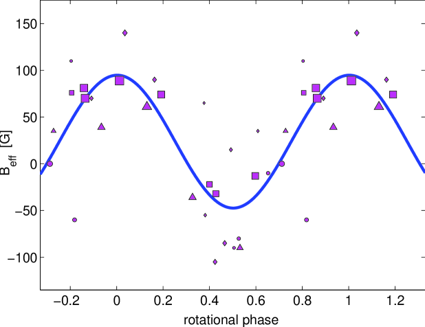
Figure 4: Effective magnetic field and its uncertainty in gauss versus rotational phase. Note that the field is extraordinarily weak and the phase of its maximum coincides exactly with the maximum of brightness. Measurements taken form: $\circ$ – Borra & Lanstreet (1980), $\Diamond$ – Bohlender & Landstreet, (1990), $\triangle$ – Donati & Semel, (1990), $\Box$ – Wade et al., (2000). Areas of individual markers correspond to the weight of the particular measurement, which is inversely proportional to the squares of their uncertainties.

4.2 Abundance anomalies and emergent flux

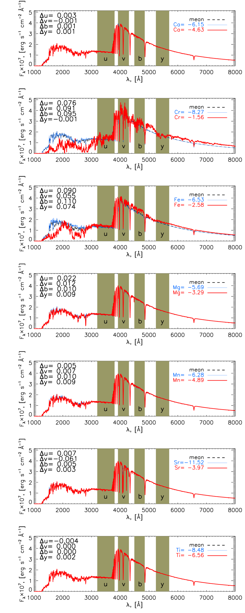
Figure 5: Effect of individual elements on the synthetic energy distribution. The difference in fluxes in Strömgren $uvby$ passbands between models computed with mean abundances and maximum abundance of the particular is presented on each plot. Fluxes were convolved with $FWHM=20$Å Gaussian for better view. The passbands (corresponding to the width of individual filter at half-maximum) of $uvby$ filters are indicated by grayed boxes.

Before presenting the results of the light curve modelling, we attempt to verify model predictions about the impact of individual elements on overall energy distribution. Figure 5 illustrates the synthetic energy distributions for models computed with maximum, minimum, and mean abundances of every element from DI maps. This exercise illustrates the maximum possible energy redistribution effect caused by enhanced chemistry inside a spot. From Fig. 5, one can note two general features. First, there are only two elements that have (on average) the strongest effect on radiative energy balance: Fe and Cr. This is mainly because they have the largest number of strong lines in the UV and thus effectively block radiation at those frequencies. Absorbed energy is then redistributed at optical wavelengths. This is illustrated by the positive delta’s of $uvby$ passbands shown on every plot. For Cr, the difference in the $y$-band between models computed with mean and maximum Cr abundance is almost zero due to the strong Cr absorption features around $5500$Å that keep fluxes almost unchanged for the highest abundance of $[\rm Cr]=-1.56$ dex. This never happens for Fe, which has a smooth flux excess in $uvby$ bands. Both elements contribute significantly to the $5200$Å flux depression frequently found in CP stars (see Kupka et al., 2003, and references therein).

Models with enhanced Mg, Mn, and Sr cause only marginal or small changes in photometric filters. Interestingly and in contrast to any other element, overabundant Sr leads to a noticeable flux deficiency in the $v$ parameter because of some very strong Sr ii $\lambda 4078,4162,4216$Å lines, while $uby$ passbands exhibit a far lower sensitivity to abundance changes (the same applies to the $v$ filter in the Ca enhanced model because of the Ca ii H & K lines, but with much smaller amplitude). This effect is even comparable to that of enhanced Fe. However, the mean abundance of Sr is only $-9.6$ and, on average, it is difficult to expect any noticeable impact of it on the resulting light curve. This is investigated in more detail later in this work. Finally, the contributions of Ca and Ti to the magnitudes of Strömgren photometry are very small.

Although the relative roles of different elements can be estimated by the aforementioned simulations, to obtain quantitative results it is still necessary to carry out accurate modelling of light curves by taking into account the individual contributions of all spotted elements.

4.3 Predicted light variation

Using DI maps of individual elements, we verified the relative contribution of each of them to the total light variation. The result is presented in Fig. 6. We note that WIRE data were smoothed over $200$ points to provide more or less a reasonable view, yet some instrumental effects are still visible.

As expected from the previous paragraph, among the seven mapped elements there are only two that strongly contribute to the amplitude of light curves in all presented photometric parameters: Fe and Cr. Next follows Mn, whose contribution can only be recognized by a keen eye (mostly in $b$ and $V$ filters). The impact of the remaining elements is negligible.

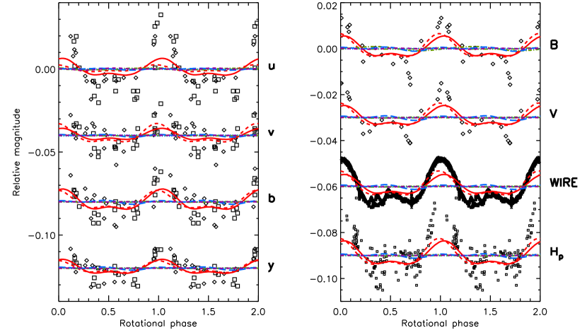
Figure 6: Differential effect of inhomogeneous surface distributions of individual elements on light variations of $\varepsilon$ UMa. Fe – full thick, Cr – dashed, Ca – dash-dotted, Mg – dash-dot-dotted, Mn – long dashed, Sr – dotted, Ti – thin dashed. Left panel: $\Box$ – Pyper & Adelman, (1985), $\Diamond$ – Musielok et al., (1980). Right panel: $\Diamond$ – Provin, (1953), $\triangle$ – Retter et al., (2004), $\Box$ – ESA, (1997). See online version for color figures.

The cumulative impact of all seven elements on the light curves of $\varepsilon$ UMa is presented in Fig. 7 (thick solid line). A very good agreement in terms of both the shape and amplitude of the light variability is found for almost all photometric bands (see Fig. 3). The only exceptions are passbands shortward of the Balmer jump, namely Strömgren’s $u$, Shemakha $U_{10},$ and $P_{10}$ for which the observed amplitude is approximately two times higher than the predicted one (see Fig. 3). In principle, this may be a signature of some other elements that were not mapped in Lüftinger et al., (2003), but still contribute to the light curve. Interestingly, a poorer fit to the $u$ passband than to others was also reported by Krtička et al., (2009) (see their Fig. 10). Nevertheless, the amplitudes in other passbands are well reproduced in both the present work and those cited above. Taking into account the large scatter in the observed points in general for the $ubvy$ system, it is difficult to explain the observed discrepancy in $u$-band in terms of impact of some missing element, at least without additional DI mapping, if ever possible. Finally, Hipparcos photometry exhibits significant scatter with a peak amplitude that is a little larger than the one theoretically predicted.

The forms of the simulated LCs agree with the observed ones very well, all of the modelled curves being systematically shifted with respect to the observed light curves by $+0\aas@@fstack{p}014$.

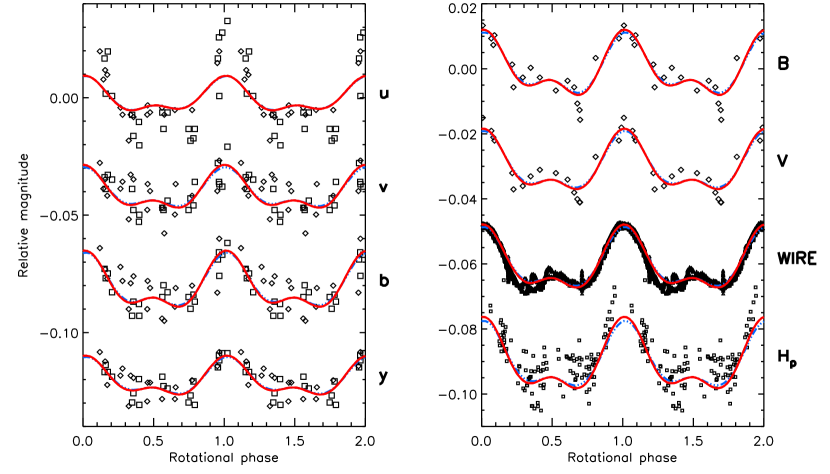
Figure 7: Same as in Fig. 6, but taking into account surface distributions of all elements simultaneously. Theoretical predictions are shown for linear (dash-dot-dotted) and quadratic limb darkening laws based on the assumptions of [M/H]=$+0.3$ (dashed), [M/H]=$0.0$ (full thick), and [M/H]=$-0.3$ (dash-dotted).

Figure 7 allows us to conclude that the inhomogeneous surface distribution of chemical elements, being derived spectroscopically with the help of DI techniques, can quantitatively describe the observed light variability detected in a number of independent photometric systems.

4.4 UV variations

As can be seen from Fig. 5, the main source of light variability is the energy redistribution from UV to visual due to the enhanced abundances of certain elements. Thus, the fluxes in these two spectral regions should display an anti-phase behaviour. This has been experimentally already reported for some CP stars (see Sokolov, 2000, 2006, for CU Vir and 56 Ari, respectively). Light curve modelling of HD 37776 and HR 7224 has also successfully predicted this characteristic signature of stellar spots.

For $\varepsilon$ UMa, we again had a problem with the lack of well-calibrated phase-resolved UV observations that could be used to study the effect of flux redistribution. The IUE archive mostly contains spectra obtained with a small aperture. This means that some of the stellar flux was missed during individual exposures, which is important to note in our study of the true variations in the continuum flux. Unfortunately, the only two spectra obtained with a large aperture (LWR06920RL and SWP07944RL) were obtained at the same rotational phase ($\varphi=0.166$).

Another possibility would be to use spectroscopic and photometric data obtained by the Copernicus OAO-2 satellite. This mission was equipped with a number of photometers in the UV and visual. The description of the photometric passbands can be found in Meade, (1999). For instance, when analysing the spectroscopic data of OAO-2 in the spectral region $1050-1830$Å, Molnar, (1975) detected significant flux variation caused by changes in line-blocking as a function of the rotational phase. An anti-phase variation in particular was reported for both spectroscopic ($1590-1690$Å) and photometric (OAO-2 $\lambda 1910$Å filter) observations relative to the optical data of Provin, (1953). Unfortunately, the available online co-added spectroscopic data from OAO-2 spectrometers contains spectra obtained at different wavelength and, even worse, at different phases. We were thus unable to choose a unique spectral region that had been observed at a sufficiently large number of rotational phases (the case would be a narrow region around $1200$Å, but only $6$ phases are available and with large errors). Nevertheless, to confirm the anti-phase behavior of the UV flux relative to the visual, we performed an exercise similar to those presented in Fig. 5 of Molnar, (1975), which illustrates the light curve of the OAO-2 $\lambda 1910$Å photometer. The predicted light curve was computed based on model fluxes in the region $1770$Å $\leq\leavevmode\nobreak\ \lambda\leavevmode\nobreak\ \leq\leavevmode\nobreak\ 2050$Å, which corresponds to the $FWHM$ of the OAO-2 S3F1 filter (see Meade, 1999). The theoretical magnitudes are shown in Fig. 8. The $V$-filter observations by Provin, (1953) are also plotted. The opposite variations in the optical and UV fluxes with respect to each other can be clearly seen. The double wave behavior of the simulated OAO-2 curve is in excellent agreement with those presented in Molnar, (1975), yet the theoretical amplitude is smaller by a factor of two. We emphasize that there is a systematical deviation between the predicted and observed magnitudes of the OAO-2 photometry, as illustrated in Fig. 3. Theoretical computations display a large scatter blueward of $\log\lambda=2.4$. At the same time, some predicted points do follow the observed linear trend of the dependence of amplitude on wavelength in UV region. This is the case for filters at $\log\lambda=2.23,2.4,2.5$. We note, however, that we did not attempt a detailed quantitative comparison between the observed and modelled light curves or their amplitudes (also because the original OAO-2 filter data, as well as the filter values, are not available online), but only confirmed the anti-phase variations in UV and optical fluxes from the modelling point of view.

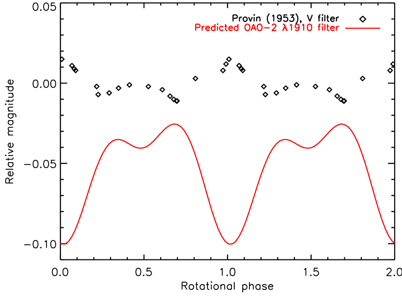
Figure 8: Simulated light curves in the region of Copernicus OAO-2 $\lambda 1910$Å filter and optical $V$-band photometry by Provin, (1953). The simulated light curve has been shifted along the y-axis for a clear visualization.

4.5 Variations in the peculiar $a$-system

The photometric parameter $a$ is often used as a measure of the peculiarity in CP stars. It was introduced by Maitzen, (1976) and corresponds to the well-known flux depression at $5200$Å frequently seen in spectra of CP stars. Using model atmosphere calculations, Kochukhov et al., (2005) noted and Khan & Shulyak, (2007) later confirmed (on the basis of more detailed computations) that Fe is the main contributor to the $5200$Å depression in the temperature range of CP stars. In addition, at low temperatures Si and Cr are also important. For HR 7224, Krtička et al., (2009) also identified the dominant role of Fe relative to Si. We carried out the same investigation and illustrate in Fig. 9 the impact of different elements on the variation in the $a$-index (note that, since the $a$-index is positive, the negative delta value in the plot correspond to the higher $a$ at corresponding phases). We thus confirm the major role of Fe, although, the contribution of Cr is very important too. Moreover, at phase $\varphi=0.7$ the contribution of Cr is comparable to that of Fe. A weak contribution of Ti can also be seen, but this fades relative to Fe and Cr. In general, the variation in the $a$-index appears to be small, on the order of a few mmag. A similar weak variation was reported for the hotter star HR 7224 (Krtička et al., 2009).

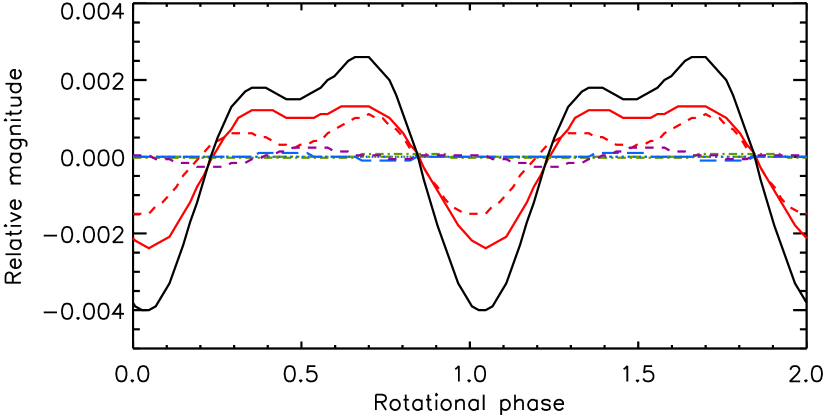
Figure 9: Impact of different elements on the light curve of the peculiar $a$ parameter. Fe – full thick, Cr – dashed, Ca – dash-dotted, Mg – dash-dot-dotted, Mn – long dashed, Sr – dotted, Ti – thin dashed. Cumulative impact of all elements is shown by the thick full thick line with highest amplitude.

4.6 Variation in hydrogen lines

We found a very small variation in the $\beta$ index on the standard system defined by Crawford & Mander, (1966) related to the Balmer H$\beta$ line, with a peak amplitude of $\approx 1.8$ mmag. This is an order of magnitude weaker than the variations reported by Musielok & Madej, (1988), and may be the signature of some additional mechanism affecting mainly profiles of hydrogen lines, as long as other photometric parameters are well fitted. For example, the rotational modulation of hydrogen lines may be caused by a non-zero magnetic pressure in the stellar atmosphere, as reported by Shulyak et al., (2010, 2007). An overview of other possible mechanisms can be found in Valyavin et al., (2004) and we refer the interested reader to this work for more details. Additional observations of the $\beta$ index from Musielok et al., (1980) have large errors and have significant scatter preventing the direct comparison with Musielok & Madej, (1988). Last but not least, the data from Musielok & Madej, (1988) contains only three points at the maximum of the $\beta$ light curve and a definite outlier at $\varphi=0.7$, which should be interpreted with caution. We thus conclude that, if true, the high amplitude of the observed variability in the $\beta$ index cannot be attributed to abundance anomalies alone.

5 Discussion

$\varepsilon$ UMa is the third CP star for which a model-based light-curve analysis predicts excellent agreement between theory and experiment, based on the assumption of the inhomogeneous surface distribution of chemical elements derived by DI techniques. The same analysis of two other and hotter Bp stars HD 37776 (Krtička et al., 2007) and HR 7224 (Krtička et al., 2009), but using slightly different methods, has also uniquely found that abundance spots may be a dominating mechanism of light variability in CP stars.

The maximum differences between the predicted and observed light curves are seen in Strömgren $u$ and Hipparcos $H_{\rm P}$ bands, as illustrated in Fig. 7. At the same time, other photometric parameters are fitted well enough to exclude any other element significantly influencing the light curves. For instance, $BV$ parameters from Provin, (1953) probably provide the closest fit, again, within the error bars of the observations (see three consecutive points at phase $1.0$, for instance). These error bars are larger for Strömgren passbands. Krtička et al., (2009) find the same larger discrepancy in $u$ but for the hotter star HR 7224. This ensures that the impact of any missed element is less significant, yet not negligible. In principle, taking into account the relative importance of different elements described in Khan & Shulyak, (2007), Si may represent such a missed element, but it could not be mapped in Lüftinger et al., (2003). The calibration of the $u$-band may also be problematic. Nevertheless, the remaining $vby$ passbands can be fitted much better without the need to involve other elements in the modelling.

As described above, to reduce computational time we decreased the resolution of the original DI maps from $2244$ surface elements to $450$. The characteristic difference in computed magnitudes between these two sets of maps was found to be $\Delta c\approx 6\times 10^{-4}$ mag, which is well below the detection limit.

The choice of the limb darkening model used to reconstruct the light curves in different photometric bands can also influence the amplitude of variations. In our study, we used a quadratic law with coefficients for every photometric band (except those described above in the paper) taken from the solar abundance model. However, neither metallicity nor the choice of limb-darkening law seem to significantly affect the light curves, nor can they explain the discrepancy in $u$. This is illustrated in Fig. 7 where, as an example, we overplot the predictions of the linear and quadratic limb darkening laws and the solar abundance model, as well as for the quadratic law with $[M/H]=+0.3$ and $[M/H]=-0.3$ models (note that the average metallicity derived from the DI maps is $[M/H]=+0.02$).

6 Conclusions

We have successfully simulated the light variability of Ap star $\varepsilon$ UMa caused by the inhomogeneous surface distribution of chemical elements detected by the DI maps of Lüftinger et al., (2003). A very close agreement in both the amplitude and shape of the light variability has been found for different and independent photometric systems. Our main conclusions are summarized below:

• The presence of abundance spots on the stellar surface is the major contributor to the light variability. We did not introduce any free parameters to improve the agreement between theory and observations.

• The light variability is due to the flux redistribution from the UV to visual region, which is initiated by the presence of abundance spots.

• We support the conclusion of Khan & Shulyak, (2007) that numerous lines of Fe and Cr are the main contributors to the well-known depression around $5200$Å.

• The variation in the theoretical $\beta$ index is very weak and approximately one order of magnitude smaller than the observed one. We thus conclude that inhomogeneous distribution of chemical elements alone cannot explain the observed light curve in the $\beta$ index.

• The strong contribution of Fe and Cr to the flux variations allows us to conclude that, as for the hotter Bp stars that have been analysed so far (HD 37776, $T_{\rm eff}=22000$ K and HR 7224, $T_{\rm eff}=14500$ K) in cooler Ap stars it is also very likely that only a few elements significantly contribute to the light variation: Fe and Cr in the case of $\varepsilon$ UMa. This must of course be tested in stars with values of $T_{\rm eff}$ lower than $T_{\rm eff}=9000$ K of $\varepsilon$ UMa.