Analysis of the MOST light curve of the heavily spotted K2IV component of the single-line spectroscopic binary II Pegasi

Abstract

Continuous photometric observations of the visible component of the single-line, K2IV spectroscopic binary II Peg carried out by the MOST satellite during 31 consecutive days in 2008 have been analyzed. On top of spot-induced brightness modulation, eleven flares were detected of three distinct types characterized by different values of rise, decay and duration times. The flares showed a preference for occurrence at rotation phases when the most spotted hemisphere is directed to the observer, confirming previous similar reports. An attempt to detect a grazing primary minimum caused by the secondary component transiting in front of the visible star gave a negative result. The brightness variability caused by spots has been interpreted within a cold spot model. An assumption of differential rotation of the primary component gave a better fit to the light curve than a solid-body rotation model.

1 Introduction

Studies of II Peg (HD 224085, Lalande 46867) began with the spectroscopic analysis of Sanford (1921). He found II Peg to be a late-type (K2), single-line spectroscopic binary (SB1) and determined its first orbital elements. Well defined, regular light variations were noticed by Chugainov (1976) who explained them by rotation of the primary component of II Peg with a cold spot on its surface. He also observed flares and concluded that this is a BY Dra-type binary system. However, subsequent photometric and spectroscopic observations by Rucinski (1977) and Vogt (1979) led these authors to conclude that the star is more akin to RS CVn-type systems, although with an invisible less-massive component; the distinguishing features of the BY Dra and RS CVn type binaries (with, respectively, dwarf and sub-giant components) were being defined at that time. Changes of equivalent width of the H_α line with orbital phase analyzed by Bopp & Noah (1980a) confirmed the RS CVn classification.

Since the 1980’s, II Peg was one of the most frequently observed RS CVn-type stars. A model of multiple spots was used for analysis of the available light-curve data sets for the first time by Bopp & Noah (1980b). The most detailed and complete study of II Peg was presented in a series of four papers by Berdyugina et al. (1998a, b, 1999a, 1999b). In the current paper we utilize most of the parameters derived in the first paper of this series which was based on high-resolution spectra used to define a high-quality radial velocity orbit. In brief, the essential physical parameters of the primary (visible) star were found to be: $T_{eff}=4,600\pm 100$ K, $\log~{}g=3.2\pm 0.2$, $[Fe/H]=-0.4\pm 0.1$, $v\,\sin i=22.6\pm 0.5$ km/s, $R_{1}=3.4\pm 0.2$ R_⊙, spectral type K2IV, with ephemeris for conjunction (visible star behind), $T_{conj}=2,449,582.9268(48)+6.724333(10)\times E$, where $E$ is an integer number of orbits.
From the analysis of TiO bands and simultaneous photometric observations, the fictitious, entirely unspotted visual magnitude of the primary star was estimated at a relatively bright level $V_{u}=6.9$; we return to this matter later in the paper as it affects the results of our spot modelling. The orbital inclination was estimated at $60^{\circ}\pm 10^{\circ}$, leading to the primary mass $M_{1}=0.8\pm 0.1$ M_⊙ and implying that the secondary star is probably a main-sequence, late-type dwarf (M0–M3V) with mass $M_{2}\approx 0.4\pm 0.1$ M_⊙. The presence of a white dwarf in this binary system was previously excluded by Udalski & Rucinski (1982) on the basis of ultraviolet observations made by the IUE spacecraft.

Berdyugina et al. (1998b) presented multi-epoch images of the primary component, obtained by means of the Doppler imaging technique. They found that the spot distribution and spot parameters obtained from the spectral analysis are in good accordance with those derived solely from analysis of photometric observations. Berdyugina et al. (1999b) discussed the “flip-flop” phenomenon, i.e. a shift of the maximum spot-activity to the opposite side of the stellar surface. The authors also concluded that – because the largest active area tends to be located on the hemisphere facing the secondary star – this component may play an important role in the magnetic phenomena in the system.

The current paper presents analysis of continuous observations of II Peg conducted using the MOST satellite during 31 days in September and October 2008 (Section 2), a circumstance which permitted us to address the following issues: (1) Study of frequency and orbital-phase localization/orientation of flares in the system (Section 3); (2) A search for grazing eclipses caused by the secondary (Section 4); (3) Determination of the differential rotation of the visible star as its minute signatures are better defined for a long observing run (Section 5).

2 Observations and data reduction

The optical system of the MOST satellite consists of a Rumak-Maksutov f/6 15 cm reflecting telescope. The custom broad-band filter covers the spectral range of 380 – 700 nm with effective wavelength falling close to Johnson’s V band. The pre-launch characteristics of the mission are described by Walker et al. (2003) and the initial post-launch performance by Matthews et al. (2004).

II Peg was observed from 15th September to 16th October 2008, in $HJD=2,454,725-2,454,756$, during 439 satellite orbits over 30.877 days. The individual exposures were 30 sec long. Only low stray-light orbital segments were used, lasting typically 25 min of the full 103 min satellite orbit. In spite of the high background, telemetry and South Atlantic Anomaly breaks, the almost continuous light curve is very well defined (Figure 1).

Figure 1: The light curve of II Peg in magnitudes. The horizontal scale is in heliocentric Julian Days (lower edge) and in orbital phase units (upper edge) with zero phase for conjunction with the visible star behind. The phases were calculated by means of the ephemeris determined by Berdyugina et al. (1998a) as given in Section 1.

Because II Peg is usually close to or slightly fainter than 7th magnitude, it was observed in the direct-imaging mode of the satellite (Walker et al., 2003). The CCD camera does not have a mechanical shutter which limits possibilities of obtaining calibration frames, as it is commonly practised during ground-based observations. However, Rowe et al. (2006a, b) proposed an excellent calibration procedure: Because the background level caused by the Earth stray light usually changes very significantly during the orbital motion of the satellite, it is possible to determine both the dark-level and the flat-field information for pixels within small images (rasters) around stars on a per-pixel basis. We removed first the background gradient visible in most frames and caused by nonuniform level of the stray light illumination and then reconstructed the dark and flat-field information for individual pixels on the basis of all available frames. The final steps were standard dark and flat-field corrections. This approach resulted in a considerable improvement of the photometric quality of the data. The implementation used our own scripts written in the IDL software environment. Aperture photometry was made by means of DAOPHOT II procedures (Stetson, 1987), as distributed by the IDL-astro library.

Figure 2: Enlargements of eight light-curve segments with eleven flares of II Peg. Groups of data points within each figure correspond to individual MOST orbits.

In spite of the above careful reductions, we still observed linear correlations between the star flux and the sky background level, most probably caused by a small photometric nonlinearity of the electronic system. The correlations showed a trend with time which could be approximated by simple linear functions of time. Corrections for the correlations produced a smooth light curve of II Peg with formal scatter of about 0.002 – 0.004 mag. However, the light curve may contain slow (10 days or longer), smooth, systematic trends at a level of about 0.01 magnitude which cannot be characterized and eliminated using the available data.

The nearby, constant, simultaneously observed stars in the unvigneted region of the CCD, GSC 02258–01385 and GSC 02258–01152, and the low amplitude ${\delta}$ Scuti-type star GSC 02258–00981, discovered by MOST, were used to determine transformations between the MOST and Johnson V magnitude systems. The $V_{T}$ and $B_{T}$ magnitudes taken from the TYCHO-2 catalogue were used, after conversion to the standard Johnson BV system. The maximum brightness magnitude of II Peg during the first half of the MOST observations was estimated at $V_{max}=7.45\pm 0.02$ (random) with the additional uncertainty of the system transformation of $\pm 0.03$ mag. We estimate that the combined uncertainty of the maximum V-magnitude of II Peg during the MOST observations does not exceed $\pm 0.06$. We note that the unspotted model prediction of Berdyugina et al. (1998a) was appreciably brighter, $V_{u}=6.9$.

We present the light curve of II Peg in Figure 1, where the V magnitudes are as determined above while the orbital phases were calculated by means of the ephemeris determined by Berdyugina et al. (1998a), as quoted in Section 1. The accumulated uncertainty of the orbital period over $E=765-769$ epochs between the original determination and the MOST observations results in a very small uncertainty of the phase, $\pm 0.002$, which can be neglected in the present context.

We note that during the MOST observations, the upper envelope of the light curve corresponding to the $V_{max}$ level slowly decreased from 7.45 to 7.46, while the amplitude of light changes, $\Delta V$, decreased from 0.145 to 0.12 magnitude. It is interesting to note that the light curve obtained by MOST is similar in its shape, maximum level and amplitude to the light curve obtained by Kaluzny (1984): $V_{max}$=7.46, $\Delta V$=0.12, as presented by Byrne et al. (1989) and Mohin & Raveendran (1993).

3 Flares

3.1 Previous observations

The astronomical literature contains a few previous reports of several very different flares observed for II Peg, including cases of non-detection even for long monitoring intervals:
(1) Bopp & Noah (1980a) observed sudden H_α enhancements which slowly decayed on time scales of days;
(2) Doyle et al. (1991) simultaneously detected a flare in X-rays and the Johnson U filter – the latter had a duration of more than 36 min;
(3) Mathioudakis et al. (1992) detected ten flares during 57.4 h of optical monitoring in the Johnson U and B filters, finding the rate of one flare per 5.9 h;
(4a) Doyle et al. (1993) observed two flares in their ultraviolet spectra, with one lasting about 3 hours;
(4b) The same work reported three optical flares, lasting 10.52, 101.00, and 9.08 min, with amplitudes 0.066 ($B$-band), 0.371 ($U$-band) and 0.207 ($U$-band) magnitude, respectively;
(5) Mohin & Raveendran (1993) found one flare in their optical spectra; they summarized the results obtained by other authors and concluded that II Peg shows a tendency to flare mainly when close to its minimum light;
(6) Henry et al. (1996) estimated a flaring rate of one flare per 4.45 h, what agrees well with the Mathioudakis et al. (1992) result. They noted that Byrne et al. (1994) monitored II Peg in 1992 in a $U$ filter and found no optical flares. Henry et al. (1996) concluded that II Peg appears to exhibit long-term changes in the level of optical flare activity;
(7) Berdyugina et al. (1999a) observed two flares in optical spectra, with rise times of a few hours, and very long decline times of 1.5 and 3 d. From H_α emission line profiles, they estimated that the flares had taken place above the visible pole, probably in connection with a large, single active region;
(8) Frasca et al. (2008) found a strong flare in spectra obtained close to light minimum, with duration time of at least 2 d.

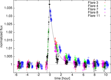
Figure 3: The mean flare made from five similar, long-lasting flares (numbers: 3, 4, 7, 8, 11), expressed in flux units. Time zero and maximum (1.037 continuum flux units) correspond to the estimated moment and mean maximum amplitude of the flare.

Figure 4: The long-lasting flare no.5 together with the subsequent flare no.6 .

3.2 MOST results

Three types of flares (Fig. 2) were detected during the MOST observations:
– Four “short” flares (nos. 1, 2, 9, 10) lasting about one or two MOST orbits (2 – 4 h), and with an amplitude of about 0.01 mag;
– Six “long” flares, very similar in shape, rise and decay time, and with amplitudes of about 0.04 mag; these flares were used to form a “mean flare” (see below);
– One particularly long-lasting flare, with duration of about one full day.
Because of the high-background data gaps at 103 min intervals and the typical MOST orbit coverage of 25 min, none of the ten flares of the first two types was observed from start to end. In particular, the four short flares could not be analyzed sufficiently thoroughly.

We attempted to construct a “mean flare” (in flux units) from the six, apparently more commonly occurring, long-duration flares, as shown in Figure 3. Because flare no.6 is affected by the preceding unusual flare no.5, we used the remaining five flares (i.e. nos. 3, 4, 7, 8, 11) for the construction. First, we expressed their intensities in contiunuum flux units (as defined by the underlying slow light variations caused by rotation of the spotted star, removed by dividing the data by low-order polynomials fitted to the quiescent parts of the light curve) and then we matched the individual flare start times manually to an uncertainty of about $\pm 2$ min. Then all flares were simply plotted together without any further scaling; the partially observed flares nos. 3 and 8 contributed only the decaying parts to such a mean flare.

The estimated rise time from the flat continuum to the maximum of the mean flare was found to be $25\pm 4$ min. The decline time, from the maximum back to the flat continuum, varied in the range of 5 to 10 h. The half-maximum duration time of the mean flare was one hour ($T_{0.5}\approx 59$ min, as defined in Kunkel (1973)) spanning the range between 50 min for flare no.8 and 74 min for flare no.7. The duration time was shorter for flare no.11, but it could not be uniquely determined from the available data. All these flares considered here most probably did not occur on the secondary component of II Peg, the M-dwarf, for which values of $T_{0.5}$ of the order of hundreds of seconds would be expected (Kunkel, 1973); the location was most likely the primary component or somewhere in the space between the stars.

In general, the first two types of flares observed by MOST, were similar to those observed before by Doyle et al. (1993) (items (4a) and (4b) in the previous section). The long-lasting flare (no.5), which started at $HJD=2,454,738.6$, close to light minimum, may be an analogue of flares observed to date as enhancements of optical spectral lines by Bopp & Noah (1980a), Berdyugina et al. (1999a) and Frasca et al. (2008). It differs markedly in its shape, rise time (6 h) and decay time (at least 18 h, possibly 24 h) from the remaining ten flares observed by MOST. It is shown among the other flares in Figure 2 and magnified in Figure 4.

The rate of eleven flares in the time span of 30.877 d gives a flaring rate of about one flare per 2.8 d. However, due to the breaks in the MOST observations, we cannot neglect the possibility of overlooking very short flares lasting only a few minutes; these would be flares similar to the two shortest observed by Doyle et al. (1993) and all of those observed by Mathioudakis et al. (1992).

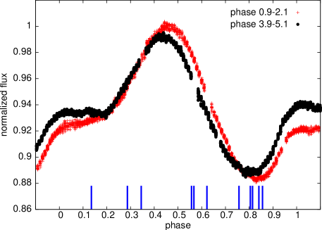
Figure 5: Individual flares are indicated by vertical marks along the horizontal (orbital phase) axis. Two sections of the light curve of II Peg, from the beginning (orbital phases 0.9 – 2.1) and the end (phases 3.9 – 5.1) of the MOST monitoring are shown for comparison. The light curve evolved mainly due to a drift in longitude of the spots at a rate faster than the orbital motion.

3.3 The phase distribution of flares

The phase distribution of flares in relation to the spot-modulated light curve can be inspected in detail in Figure 5. The flares appear not to be uniformly distributed in orbital phase: as many as five flares appeared within the light minimum, in the orbital phase interval 0.75 – 0.85. This supports the conclusion of Mohin & Raveendran (1993) that flares in II Peg are concentrated close to light minimum when the most heavily spotted side of the visible star is directed toward the observer. However, a Kolmogorov–Smirnov test for the deviation of the phase distribution from uniformity gave the probability that the distributions appear to be identical of 0.28. While this is a small number, it is not small enough to prove this assertion, which still requires confirmation.

4 A search for eclipses

High-precision photometry from space carries a potential for detection of eclipses caused by transits of the undetected secondary companion over the visible star. We estimated the expected depths and durations of primary eclipse in the Johnson V-band for several values of inclination using the Wilson-Devinney light curve synthetic code (Wilson, 1996) for the physical parameters obtained by Berdyugina et al. (1998a); this is shown in Fig. 6 and Fig. 7

A careful inspection of the MOST data revealed no indication of any eclipses, as can be seen in Figure 7. To analyze the conjunction segments of the light curve, trends introduced by spots were fitted within phase ranges 0.93 – 0.97 and 1.03 – 1.07 and then normalized light curves were analyzed in great detail. The data do not reveal any systematic, localized deviations which would have depths similar to those predicted in Fig. 6 to less than 0.1 per cent.

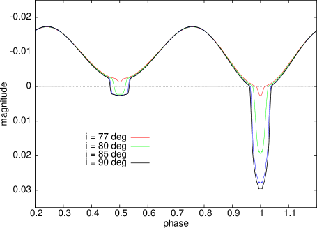
Figure 6: Synthetic light curves for II Peg computed using the stellar parameters obtained by Berdyugina et al. (1998a) for four different values of the orbital inclination.

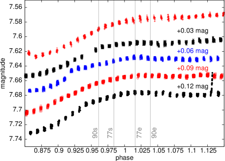
Figure 7: Segments of the MOST data close to predicted times of primary eclipse. The segments for four consecutive conjunctions (which show spot evolution in time) have been shifted down for clarity by the indicated magnitude amounts; the first conjunction is on top. The start (90s, 77s) and end (77e, 90e) phases of the eclipse, estimated for $i=90^{\circ}$ and $i=77^{\circ}$ are represented by four vertical lines. Note that, as discussed in Sec. 2, the current spectroscopic ephemeris is very accurate and predicts the conjunction phase to $\pm 0.002$.

Table 1: Results of the light curve models for a rigidly and a differentially rotating star for $i=60^{\circ}$. The ranges in resulting parameters for the two extreme values of the normalization parameter $F_{u}$, 1.19 and 1.33 (see the text) are given in brackets as estimates of parameter uncertainties.
a – assumed as constant during modelling,
b – determined using the constraints $R_{1}=3.4$ R_⊙ and $v\sin i=22.6$ km/s,
c – calculated using Eq.(1).

Prox. effects:	neglected (1)	neglected (2)	accounted (3)	accounted (4)
$F_{u}$	$1.26\pm 0.07^{a}$	$1.26\pm 0.07^{a}$	$1.26\pm 0.07^{a}$	$1.26\pm 0.07^{a}$
$k$	—	0.022 (0.033-0.021)b	—	0.0245 (0.04-0.0225)b
$P_{eq}~{}[d]$	—	$6.5940\pm 0.0005^{b}$	—	$6.5940\pm 0.0005^{b}$
$p_{1}~{}[d]$	6.6641 (6.6651 – 6.6635)	6.6748 (6.6684 – 6.6776)c	6.6733 (6.6738 – 6.6729)	6.6850 (6.6808 – 6.6867)c
$t_{1}~{}[hjd]$	25.903 (25.900 – 25.903)	25.534 (25.661 – 25.497)	25.824 (25.839 – 25.821)	25.535 (25.665 – 25.499)
${\phi}_{1}~{}[^{\circ}]$	74.2    (67.1 – 78.3)	47.9    (36.8 – 50.5)	71.9    (66.0 – 76.6)	48.2    (34.7 – 51.7)
$r_{1}~{}[^{\circ}]$	31.4    (24.8 – 39.9)	20.5    (17.9 – 21.7)	31.1    (25.8 – 39.5)	22.4    (18.8 – 24.4)
$p_{2}~{}[d]$	6.6641 (6.6651 – 6.6635)	6.7331 (6.7432 – 6.7309)c	6.6733 (6.6738 – 6.6729)	6.7429 (6.7484 – 6.7374)c
$t_{2}~{}[hjd]$	28.589 (28.509 – 28.641)	28.018 (27.912 – 28.057)	28.596 (28.539 – 28.645)	28.166 (28.045 – 28.220)
${\phi}_{2}~{}[^{\circ}]$	18.1    (13.6 – 21.3)	75.7    (55.0 – 79.7)	21.2    (17.7 – 24.4)	71.7    (49.1 – 76.6)
$r_{2}~{}[^{\circ}]$	15.0    (14.6 – 15.4)	27.4    (15.5 – 36.3)	16.5    (16.0 – 17.2)	26.4    (15.6 – 34.9)
$p_{3}~{}[d]$	—	—	—	—
$t_{3}~{}[hjd]$	—	—	—	—
${\phi}_{3}~{}[^{\circ}]$	-90a	-90a	-90a	-90a
$r_{3}~{}[^{\circ}]$	89a	89a	89a	89a
${\chi}^{2}_{red,weigh}$	13.79	11.75	14.72	12.28

5 Light curve analysis

In this investigation we modeled the MOST light curve in terms of dark spots which are internally invariable in time. We used the program StarSpotz, which was successfully applied to ${\epsilon}~{}Eri$ (Croll et al., 2006) and ${\kappa^{1}}~{}Cet$ (Walker et al., 2007), where differential rotation of the stars was found. The reader is directed to these papers for details of the model. The program is based on the program SpotModel (Ribárik, 2002) which utilizes the analytical models developed by Budding (1977) and Dorren (1987).

The assumption of the internal invariability of spots is most likely not fulfilled in the case of II Peg. As Doppler images obtained during 1994–2002 reveal (Berdyugina et al., 1998b, 1999b), the spots may constantly change their properties over time, in time scales of several rotation periods. The shortest time scales for appreciable spot changes could be as short as 2 months, which is comparable with the length of the MOST run of 31 days. The global, progressive light curve shape changes (Fig. 1) can be easily explained by differential rotation of the stellar surface with small, random changes of the spots well averaged over the time of observations.
A more detailed investigation of differential rotation should be supported by simultaneous high-resolution spectroscopic observations. Without them, as in the current investigation, we are unable to assert whether spots really remained sufficiently constant during the MOST observations. Additionally, whatever method of spot shape restoration is used (including the maximum entropy method), the results will always be subject to limitations imposed by the instrumental effects mentioned in Section 2.

5.1 Light curve modelling

After first trial runs it turned out that at least two cold spots on the hemisphere directed to the observer are necessary to give a reasonable explanation of the light variations.
Compatible with the non-detection of eclipses, we assumed: $i=60^{\circ}$, $R_{1}=3.4$ R_⊙ and $v\sin i=22.6$ km/s, as determined by Berdyugina et al. (1998a) (see also fig. 6 of their paper). Also, as fixed parameters for the light curve models, we assumed the linear limb-darkening coefficient $u=0.817$, adopted using the tables of Díaz-Cordovés et al. (1995). We also fixed the photospheric and spot temperatures at $T_{phot}=4,600$ K and $T_{spot}=3,600$ K, as based on the results of Berdyugina et al. (1998b, 1999b). This assumption was required to fix the spot-to-photosphere flux ratio $f$ for the bandpass of the MOST observations. $f=0.077\pm 0.015$ has been evaluated by means of the SPECTRUM programme (Gray, 2001) and Kurucz’s atmosphere models (Kurucz, 1993) using the MOST filter bandpass. The same value of $f$ was assumed for all spots. The remaining parameters of the model were, for each spot: (1) the initial moment $t$ (in $hjd\equiv HJD-2,454,700$), when the spot is exactly facing the observer, (2) the rotation period of the spot $p$ in days, (3) the latitude ${\phi}$, (4) the diameter $r$ in degrees and (5) the value of unspotted flux $F_{u}=1.26$.
The latter value was calculatted assuming the value of unspotted magnitude equal to $V_{u}=7.20$, as determined by Chugainov (1976) at the time when he observed a flat maximum, and also adopted by Mohin & Raveendran (1993). We note that Berdyugina et al. (1998b) suggested $V_{u}=6.9$, but for such a high brightness it is impossible to obtain a physically plausible fit to the light curve: We would have to postulate that we observed II Peg with almost the whole surface covered by black spots. As we described in Section 2, we observed $V_{max}=7.45\pm 0.06$, based on the MOST instrumental system, after transformation to the V-band using nearby stars. If the unspotted magnitude for II Peg is $V_{u}=7.20$, the unspotted flux at the time of the MOST observations would be $F_{u}=1.26\pm 0.07$ (using normalization of $F_{u}=1$ for $V_{max}=7.45$). This leads however to the difficulty of large radii of both spots with some overlap, which is not admitted by the model. We solved this problem assuming a third, very large ($r_{3}=89^{\circ}$) circular spot, covering practically the whole hemisphere directed away from the observer. This spot remained constant and – because of the low inclination – only partially visible. It represented the non-variable part of the spotted photosphere. This assumption is strongly supported by results obtained from the Doppler imaging technique: According to Neff et al. (1995), O’Neal & Neff (1997), Marino et al. (1999) and O’Neal et al. (1998) spots are always visible and they cover between 35 to 64 per cent of the hemisphere projected toward the observer. As mentioned in Section 2, the amplitude of light changes observed by MOST was $\Delta V=0.145-0.12$ magnitude. This was close to the smallest value noticed to date which, according to Mohin & Raveendran (1993), means that during the MOST observations spots covered a large fraction of the stellar surface.

The light curve used in the model utilized mean points formed for individual MOST orbits, after removal of all stellar flares. Typically 40 – 70 points contributed to one MOST-orbit average point. The formal normalized flux errors ($\sigma$) per point is about 0.0011 (median) and the full range of 0.0007 – 0.0022. Please note, that as discussed in Section 2, the light curve may contain a roughly 10 day-long smooth trend, a few times larger in amplitude than the formal normalized flux errors given above.

The spot model using the StarSpotz program assumes spherical stars. II Peg is a binary system where some light modulation is expected from ellipsoidal and reflection effects, so-called proximity effects. They are small in an absolute sense (less than 0.02 mag, see Figure 6) but cannot be neglected as, for the assumed $i=60^{\circ}$, they reach almost 9 per cent (0.012 mag) of the observed spot-modulation amplitude. Because of the uncertainty with the inclination ($\pm 10^{\circ}$), all physical parameters of II Peg are not fully known; this affects predictions of the proximity effects. To assess the impact of the proximity effects on the final results, particularly on the differential rotation of the visible star, we used two light curves, corrected and uncorrected for the proximity effects. Each of the two light curves was analyzed assuming a rigidly and a differentially rotating stellar surface.

The individual spot rotation periods $p_{1,2}$ were assumed to depend on the stellar latitude $\phi_{1,2}$, the rotational period on the equator $P_{eq}$ and differential rotation coefficient $k$ through:

$$p_{i}({\phi_{i}})=P_{eq}/(1-k\sin^{2}{\phi_{i}}),$$ (1)

where i=1,2.
The search procedure for $k$ consisted of two steps: first, for the assumed $R=3.4$ R_⊙, the proper value of $P_{eq}=6.5940\pm 0.0005$ d was found, providing the observed $v\,\sin i=22.6$ km/s; then – for the value of unspotted flux level $F_{u}=1.26$ – the differential rotation coefficients $k$, returning the smallest value of the reduced and weighted ${\chi}^{2}$ was derived. The formula given by Eq.(1) corresponds to the solar-type differential rotation law. Due to the low quality of our fits, most probably dominated by the inadequacies of the spot model (see Section 5.2), we did not consider other possible types of differential rotation.

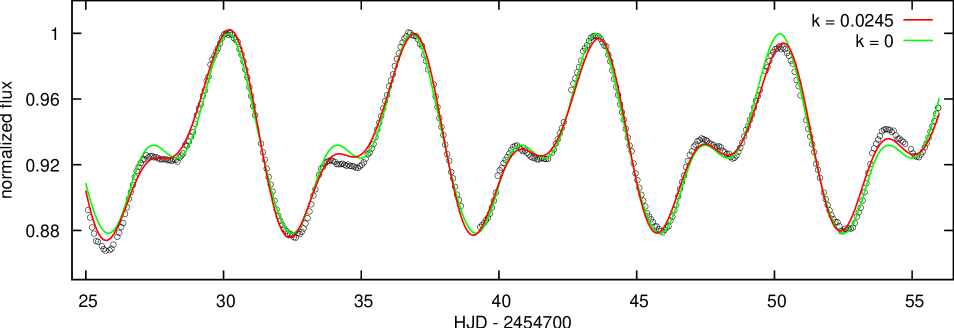
Figure 8: The fit to the light curve of II Peg (corrected for proximity effects) by the model with solid-body rotation ($k=0$, column 3 of Table 1) and with differential rotation ($k=0.0245$, column 4).

5.2 Results of the light curve modelling

The results of modelling are presented in Table 1. One can see in Figure 8 that the fit obtained for the case of differential rotation describes the light curve better than the solid-body rotation model. This applies to the general light curve evolution, and in particular to the progressive amplitude decrease, as discussed in Section 2. We also note that only for the differential-rotation models does the larger spot face the secondary star, similarly as obtained by Berdyugina et al. (1998b, 1999b).

To estimate the systematic errors of our models resulting from the large uncertainty of $V_{max}$ of $\pm 0.06$ mag, we repeated our solutions for two values of the unspotted flux level, $F_{u}=1.19$ and $F_{u}=1.33$. This choice affects the solutions strongly and the resulting spread in parameters can be taken as an indication of the uncertainty in our solutions. Note that the order in the range limits given in Table 1 is sometimes inverted but the first value always corresponds to the smaller value of $F_{u}$.

In general, the residuals – typically at a level of 0.004 of the mean flux – are much larger than formal errors of individual data points (typically 0.001). This has driven values of the formally derived, reduced, weighted $\chi^{2}$ (Table 1) to values well above unity indicating systematic trends in residuals, most probably reflecting the difference between the true and the circular shape of spots which was assumed in the model.
Because of the dominance of the systematic deviations over the random noise in the values of $\chi^{2}$, this parameter has only an indicative utility. Nevertheless, for each pair of solutions, with included (columns 3, 4) or excluded (columns 1, 2) proximity effects, the differential-rotation solution appears to be always better than the solid-rotation one. Taking these considerations into account, we select the solution in the last column of Table 1 as the final one, and we plot it in Figure 8.

5.3 Comparison with other results

Henry et al. (1995) determined the differential rotation parameter, $k=0.005\pm 0.001$, for II Peg using several multi-epoch light curves. Our result of $k=0.0245_{-0.0020}^{+0.0155}$ is in better accordance with the linear relation between parameters of RS CVn-type stars (Eq. 9 in Henry et al. (1995)): $\log k=-2.12(12)+0.76(6)\times\log P_{rot}-0.57(16)\times F$, where $F=R_{star}/R_{Roche}$. Using the parameters listed in Table 1, we have $P_{rot}\approx 6.7$ d, $F=3.4/7.1\approx 0.48$, leading to a prediction of $k=0.017$. However, when we take into account the scatter visible in fig. 28 of Henry et al. (1995), a broad range of $0.002<k<0.066$ is admitted for this value of $P_{rot}$. Interestingly, the value of $k$ determined in this paper for II Peg is similar to that estimated for the apparently single, but even faster rotating giant, FK Com ($k=0.016$ for $P=2.4$ d) by Korhonen et al. (2002).

6 Conclusions

Analysis of the almost-continuous, one month-long photometric monitoring of II Pegasi by the MOST satellite permits us to formulate the following conclusions:

1. Eleven flares were observed, one lasting about 24 h and six flares moderately long, lasting typically 5 to 10 hours. The characteristics of the four shortest flares were difficult to estimate.

2. The primary eclipse of the visible star by its companion (probably M-dwarf) was not detected, which gives an upper limit for the orbital inclination of the system of $76^{\circ}$.

3. From the analysis of the dark-spot modulated light curve, assuming $i=60^{\circ}$, $R_{1}=3.4$ R_⊙, $v\sin i=22.6$ km/s (Berdyugina et al., 1998a) and absence of internal variability of spots during the MOST observations, we obtained an estimate of the parameter measuring the differential rotation of the primary component of II Peg: $k=0.0245^{+0.0155}_{-0.0020}$. The error of $k$ reflects the major uncertainty in the unspotted brightness of the star so that the value of $k$ remains preliminary; it will improve with future ameliorations in values of the assumed stellar parameters which enter the model.

References

- Bopp & Noah (1980a) Bopp B.W., Noah P.V., 1980a, PASP, 92, 333
- Bopp & Noah (1980b) Bopp B.W., Noah P.V., 1980b, PASP, 92, 717
- Berdyugina et al. (1998a) Berdyugina S.V., Jankov S., Ilyin I., Tuominen I., Fekel F.C., 1998a, A&A, 334, 863
- Berdyugina et al. (1998b) Berdyugina S.V.,Berdyugin A.V., Ilyin I., Tuominen I., 1998b, A&A, 340, 437
- Berdyugina et al. (1999a) Berdyugina S.V., Ilyin I., Tuominen I., 1999a, A&A, 349, 863
- Berdyugina et al. (1999b) Berdyugina S.V., Berdyugin A.V., Ilyin I., Tuominen I., 1999b, A&A, 350, 626
- Budding (1977) Budding E., 1977, Ap&SS, 48, 207
- Byrne et al. (1989) Byrne P.B., Panagi P., Doyle J.G., Englebrecht C.A., McMahan R., Marang F., Wegner G., 1989, A&A, 214, 227
- Byrne et al. (1994) Byrne P.B., Lanzafame A.C., Sarro L.M., Ryans R., 1994, MNRAS, 270, 427
- Chugainov (1976) Chugainov P.F., 1976, Krymskaia Astrof. Obs., Izvestiia, 54, 89
- Croll et al. (2006) Croll B., Walker G., Kuschnig R., Matthews J., Rowe J., Walker A., Rucinski S., Hatzes A., Cochran W., Robb R., Guenther D., Moffat A., Sasselov D., Weiss W., 2006, ApJ, 648, 607
- Díaz-Cordovés et al. (1995) Díaz-Cordovés J., Claret A., Giménez A., 1995, A&AS, 110, 329
- Dorren (1987) Dorren J.D., 1987, ApJ, 320, 756
- Doyle et al. (1991) Doyle J.G., Kellett B.J., Byrne P.B., Avgoloupis S., Mavridis L.N., Seiradakis J.H., Bromage G.E., Tsuru T., Makishima K., McHardy I.M., 1991, MNRAS, 248, 503
- Doyle et al. (1993) Doyle J.G., Mathioudakis M., Murphy H.M., Avgoloupis S., Mavridis L.N., Seiradakis J.H., 1993, A&A, 278, 499
- Frasca et al. (2008) Frasca A., Biazzo K., Tas G., Evren S., Lanzafame A.C., 2008, A&A, 479, 557
- Gray (2001) Gray R.O., 2001, http://phys.appstate.edu/spectrum/spe- ctrum.html, Department of Physics and Astronomy, Appalachian State University
- Henry et al. (1995) Henry G.W., Eaton J.A., Hamer J., Hall, D.S., 1995, ApJSS, 97, 513
- Henry et al. (1996) Henry G.W., Newsom M.S., 1996, PASP, 108, 242
- Kaluzny (1984) Kaluzny J., 1984, IBVS, No. 2627
- Korhonen et al. (2002) Korhonen H., Berdyugina S.V., Tuominen I., 2002, A&A, 390, 179
- Kunkel (1973) Kunkel W.E., 1973, ApJSS, 213,25
- Kurucz (1993) Kurucz R., 1993, Atomic data for opacity calculations. Kurucz CD-ROM No. 1.–18., Cambridge Mass., Smithsonian Astrophysical Observatory
- Marino et al. (1999) Marino G., Rodonò M., Leto G., Cutispoto G., 1999, A&A, 352, 189
- Matthews et al. (2004) Matthews J.M., Kusching R., Guenther D.B., Walker G.A.H., Moffat A.F.J., Rucinski S.M., Sasselov D., Weiss W.W., 2004, Nature, 430, 51
- Mathioudakis et al. (1992) Mathioudakis M., Doyle J.G., Avgoloupis S., Mavridis L.N., Seiradakis J.H., 1992, MNRAS, 255, 48
- Mohin & Raveendran (1993) Mohin S., Raveendran A.V., 1993, A&A, 277, 155
- O’Neal & Neff (1997) O’Neal D., Neff J.E., 1997, AJ, 113, 1129
- O’Neal et al. (1998) O’Neal D., Saar S.H., Neff J.E., 1998, ApJ, 501, L73
- Neff et al. (1995) Neff J.E., O’Neal D., Saar S.H., 1995, ApJ, 452, 879
- Udalski & Rucinski (1982) Udalski A., Rucinski S.M., 1982, AcA, 32, 315
- Ribárik (2002) Ribárik G., 2002, Occasional Technical Notes from Konkoly Observatory, No.12
- Rucinski (1977) Rucinski S.M., 1977, PASP, 89, 280
- Rowe et al. (2006a) Rowe J.F., Matthews J.M., Kusching R., et al., 2006a, Mem S.A.It., 77, 282
- Rowe et al. (2006b) Rowe J.F., Matthews J.M., Seager S., et al., 2006b, ApJ, 646, 1241
- Sanford (1921) Sanford R.F., 1921, ApJ, 53, 201
- Stetson (1987) Stetson P.B., 1987, PASP, 99, 191
- Vogt (1979) Vogt S.S., 1979, PASP, 91, 616
- Walker et al. (2003) Walker G., Matthews J., Kuschnig R., Johnson R., Rucinski S., Pazder J., Burley G., Walker A., et al., 2003, PASP, 115, 1023
- Walker et al. (2007) Walker G., Croll B., Kuschnig R., Walker A., Rucinski S., Matthews J., Guenther D., Moffat A., Sasselov D., Weiss W., 2007, ApJ, 659, 1611
- Wilson (1996) Wilson R.E., 1996, Documentation of Eclipsing Binary Computer Model