M Dwarf Flares from Time-Resolved SDSS Spectra

Abstract

We have identified 63 flares on M dwarfs from the individual component spectra in the Sloan Digital Sky Survey using a novel measurement of emission line strength called the Flare Line Index. Each of the $\sim$38,000 M dwarfs in the SDSS low mass star spectroscopic sample of West et al. was observed several times (usually 3-5) in exposures that were typically 9-25 minutes in duration. Our criteria allowed us to identify flares that exhibit very strong H$\alpha$ and H$\beta$ emission line strength and/or significant variability in those lines throughout the course of the exposures. The flares we identified have characteristics consistent with flares observed by classical spectroscopic monitoring. The flare duty cycle for the objects in our sample is found to increase from 0.02% for early M dwarfs to 3% for late M dwarfs. We find that the flare duty cycle is larger in the population near the Galactic plane and that the flare stars are more spatially restricted than the magnetically active but non-flaring stars. This suggests that flare frequency may be related to stellar age (younger stars are more likely to flare) and that the flare stars are younger than the mean active population.

1 Introduction

Flares are explosive events caused by magnetic reconnection in stellar atmospheres (Haisch et al., 1991, and references therein). In the standard model, electrons are accelerated along magnetic field lines and impact the lower stellar atmosphere. This catastrophic release of magnetic energy causes emission from the radio to the X-ray (Hawley et al., 1995, 2003; Osten et al., 2005; Fuhrmeister et al., 2007; Berger et al., 2008). On M dwarfs, the most distinct observational characteristic is the tremendous increase in the blue and near-ultraviolet continuum emission, up to several magnitudes in a few minutes or less (Hawley & Pettersen, 1991; Eason et al., 1992; Kowalski et al., 2010). The initial burst, or impulsive phase, is also characterized in the optical spectrum by increases in chromospheric line emission, particularly in the hydrogen Balmer lines (Hawley & Pettersen, 1991; Martín & Ardila, 2001; Fuhrmeister & Schmitt, 2004). The impulsive phase is followed by a gradual decay phase which can last from tens of minutes to hours for the largest flares (Moffett, 1974; Zhilyaev et al., 2007).

The rate at which flares occur is of significant current interest. Recently, numerous planets have been discovered around M dwarfs, including some of only a few Earth masses (Udry et al., 2007; Charbonneau et al., 2009; Forveille et al., 2009; Mayor et al., 2009; Correia et al., 2010). The atmospheres of these planets may be greatly affected by the amount of high-energy radiation incident upon them. Cool, red M dwarfs produce little high-energy radiation during quiescence, so the flaring rate is an important factor in determining planet habitability (Heath et al., 1999; Segura et al., 2005; Tarter et al., 2007; Walkowicz et al., 2008; Segura et al., 2010).

Additionally, characterizing the M dwarf flaring rate is important for new instruments such as Pan-STARRS (Kaiser, 2004), the Palomar Transit Factory (Rau et al., 2009) and the Large Synoptic Survey Telescope (LSST Science Collaborations: Paul A. Abell et al., 2009), which will carry out large, all-sky surveys in the time-domain. Effectively selecting rare, exotic transients from the large sample of M dwarf flares that will be observed in these surveys requires reliable knowledge of expected flare characteristics and rates.

Traditionally, the frequency of flares on M dwarfs has been determined through time-resolved photometric monitoring of individual stars. Lacy et al. (1976) and Gershberg & Shakhovskaia (1983) have amassed several hundred hours of optical observations on dozens of the most magnetically active and well-known flare stars and have derived power law relationships between the total energy in the U band and the frequency of a flare, with less energetic flares occurring more frequently. Studies on individual stars have confirmed the power law form of the frequency distribution, albeit with a range of exponents (Walker, 1981; Pettersen et al., 1984; Robinson et al., 1995; Leto et al., 1997; Robinson et al., 1999). At ultraviolet wavelengths, Audard et al. (2000) and Sanz-Forcada & Micela (2002) found that the EUVE flare frequency distributions for active stars also had a power law form. In addition, Audard et al. (2000) demonstrated that large flares occur preferentially on the X-ray brightest stars.

Spectroscopic studies of flares have also investigated the flare rate, but with smaller samples and incomplete information on flare energies it is not possible to compute the flare frequency distribution as described above for photometric data. Instead the results are usually presented as “flare duty cycles”, meaning that during the entire period of observation, flares occur during a certain percentage of the time. Alternatively a “flare rate” (number of flares per hour) is sometimes given, but without reference to the energy distribution of the flares. Both the flare duty cycle and flare rate are strong functions of the observational sample, since such factors as the individual exposure time (compared to the typical flare timescale), the flare visibility in the line radiation compared to the continuum, and the flare energy will all be important in determining whether a particular observation is counted as flaring.

Reid et al. (1999) estimated a duty cycle of 7% from H$\alpha$ observations of the M9.5 dwarf BRI 0021-0214, while Crespo-Chacón et al. (2006) observed 14 small flares on AD Leonis, none of which produced measurable continuum increase, and determined a flare rate of $>0.7\mbox{ flares}/\mbox{hr}$. Schmidt et al. (2007) investigated a sample of 81 M dwarfs, each observed a few times and found a flare duty cycle of $\sim$5%, based on H$\alpha$ variability. Recently, Lee et al. (2010) reported a duty cycle of $\lesssim$ 5% for H$\alpha$ flares (defined as a brightness increase of a factor of ten) from time-resolved spectroscopic monitoring ($\sim$1 hour each) of 43 M dwarfs.

The small numbers of stars in most previous studies (both photometric and spectroscopic) did not allow examination of whether the flare rate is a function of stellar or Galactic parameters. However, Kowalski et al. (2009) used the repeat observations from the SDSS Stripe 82 photometry ($\sim$60 epochs per object spread over 10 years) to identify flares and determine flare rates. They identified 271 flares on more than 50,000 M dwarfs, a sample which is orders of magnitude larger than previous work and the first to contain significant numbers of both magnetically active and inactive stars. The vast majority of flares (but not all) in the Kowalski et al. (2009) study occurred on active stars, and they found that the flare star spatial distributions reflect the active star distributions as a function of spectral subtype (West et al., 2008).

It should be clear that the flare rates, flare duty cycles, and flare frequency distributions described above are distinctly different measurements, and are difficult to compare. In addition, the criteria used to define a flare differ depending upon the method of observation (photometry vs spectroscopy), the exposure time during which a flare may occur (resolved vs unresolved), the wavelength (optical vs near-ultraviolet), and the emission mechanism (continuum vs lines). The sample selection (spectral type distribution, Galactic height distribution, color selection, etc.) also has a strong influence on the number of flares found. Additionally, flares themselves are not homogeneous. Flares with the same energy exhibit apparent magnitude variations that depend on the brightness of the star during quiescence (the so-called “contrast” effect). On stars with the same quiescent brightness, flares of the same energy exhibit a wide range of light curve shapes, with some flares rising and decaying quickly, giving large changes in apparent magnitude, while others are slower, with smaller peak magnitude. Understanding how often an M dwarf is seen in a flaring state requires knowledge of many stellar, flare, and sample properties.

Spectroscopic flare data typically have longer exposure times, may contain unresolved flares, are usually at optical wavelengths, and are more likely to observe flares, especially small ones, through enhanced line emission. Flare rates and frequency distributions are therefore not good descriptions of the data, and we will use the flare duty cycle (the fraction of epochs classified as flares) in this work.

Here we present the first large, statistical study of spectroscopic flare duty cycles. The low mass stars in this study are taken from the Sloan Digital Sky Survey Data Release 5 (SDSS DR5; Adelman-McCarthy et al., 2007) low-mass star spectroscopic sample (West et al., 2008), which consists of over 38,000 objects between spectral types M0 and L0. All SDSS spectra are the result of coadding several (usually 3-5) individual exposures, typically (but not always) observed on the same night. The individual component exposure times were generally between 9 and 25 minutes. The individual spectra were made public as part of the SDSS Data Release 6 (Adelman-McCarthy et al., 2008). The repeated, shorter exposures are used to aid in cosmic ray rejection for the final combined SDSS spectrum. However, these repeat spectra can be used to examine the time variability of spectral features. We take advantage of the time sampling contained in the individual exposures to identify flares based on the strength and variability of spectral lines.

We have created a unique tool we use to identify flares: the Flare Line Index (FLI), which allows us to quantitatively measure spectral line strength in low signal-to-noise (SNR) spectra, where equivalent width measurements are not possible. We then used False Discovery Rate analysis (Miller et al., 2001) to identify flares based on exceptionally strong emission line strength. Additionally, we used FLI variability criteria to identify flares based on changes in emission line strength over the course of the exposures.

In §2 we further characterize our sample and describe our quality cuts. The tools for our analysis are described in detail in §3. The flare selection criteria are defined in §4, and the results are presented in §5. Finally, we conclude in §6.

2 The Sample

We began with the SDSS DR5 low-mass star sample of West et al. (2008), for which low mass stellar candidates were chosen from the SDSS DR5 spectroscopic catalog using the photometric color selection $r-i>0.53$ and $i-z>0.3$, along with a standard set of SDSS processing flags (SATURATED, BRIGHT, NODEBLEND, INTERP_CENTER, BAD_COUNTS_ERROR, PEAKCENTER, NOTCHECKED, and NOPROFILE were all required to be zero). Stars with $r$-band extinction $>$ 0.5, colors consistent with having a white dwarf companion (Smolčić et al., 2004), or measured radial velocity $>$ 500 km s^-1 were culled from the sample (see West et al. (2008) for more details).

The 38,717 spectra of individual objects in the DR5 sample that meet the above criteria consist of 142,032 individual exposures that were made available in DR6. The distribution of number of exposures per object and the exposure times are shown in Figure 1. Although most of the spectra for an object were observed consecutively on a single night, 27% of objects have additional exposures separated by two hours or more.

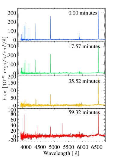
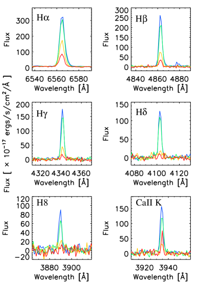
Figure 2: A sequence of spectra of a typical decay phase flare (left), with the time in minutes from the beginning of the first exposure. A detailed look at the emission lines (right, color corresponding to the exposure number on the left) reveals that H$\alpha$ and H$\beta$ remain in emission longer than the higher-order Balmer lines. Note that Ca II K increases during the third exposure, an effect not observed in the Balmer lines.

The SDSS spectra have wavelength coverage from 3800 to 9200 Å, and resolution ranging from 1800 to 2200. We therefore were able to measure five hydrogen Balmer lines (H8, H$\delta$,H$\gamma$, H$\beta$, H$\alpha$), as well as Ca II K. Ca II H and H$\epsilon$ are blended at this resolution and are not considered in our analysis. The wavelength regions used for the continuum and line regions are given in Table 1 (cf. Bochanski et al., 2007). An example of the data, Figure 2 shows the four exposures and line profiles from the six measured lines of a typical decay phase flare.

Table 1: Line and continuum regions

Line	Line Region (Å)	Continuum 1 (Å)	Continuum 2 (Å)
H8	3884.15 - 3898.15	3850 - 3880	3910 - 3930
Ca II K	3928.66 - 3938.66	3910 - 3925	3950 - 3960
H$\delta$	4097.00 - 4110.00	4030 - 4080	4120 - 4170
H$\gamma$	4331.69 - 4350.00	4270 - 4320	4360 - 4410
H$\beta$	4855.72 - 4870.00	4810 - 4850	4880 - 4900
H$\alpha$	6557.61 - 6571.61	6500 - 6550	6575 - 6625

2.1 Quality Cuts

2.1.1 Cosmic Rays

Cosmic Rays (CRs) were not removed from the individual component spectra in the SDSS DR6 spectroscopic pipeline, but individual pixels that contained likely CRs were flagged. We visually inspected many of the flagged pixels and found that the pipeline routines frequently misidentified stellar emission lines as CRs. Since flares produce strong and time variable emission that might be misclassified as CRs, we developed a separate criterion to identify pixels as CRs in the line regions, so as not to reject genuine emission: a pixel within the line region was called a CR if the difference between that pixel and the continuum level was more than ten times the standard deviation of the other pixels in the region. Our criterion identified CRs in the H$\alpha$ and H$\beta$ line regions in 0.55% and 0.69% of spectra respectively, as compared to 2.7% and 3.5% of the spectra that the SDSS pipeline flags identified. There were no significant variations in the rate of CRs detected at different spectral subtypes using either definition.

Although this criterion still allows some CRs to remain undetected and masquerade as emission lines, we require emission in both H$\alpha$ and H$\beta$ to identify an object as in a flaring state (see §4). This requirement greatly reduces the contamination by CRs, since two independent CR strikes on H lines in the same spectrum happen very rarely. Using the SDSS CR flags, we found that a “CR” is detected in both the H$\alpha$ and H$\beta$ regions in 0.3% of the spectra, compared to 0.007% with our CR criterion. All of the objects that met our flare criteria were inspected by eye, ensuring that no CRs led to an incorrect flare classification. Since the continuum regions are much wider than the line regions and are only used as an indicator of the continuum level and signal-to-noise ratio (SNR), we used the more conservative SDSS CR flags to mask any suspect pixels in all calculations involving the continuum regions.

2.1.2 Sample Separation by Signal-to-Noise Ratio

The large sample size allowed us to divide our objects into 3 quality bins based on the SNR. Because M dwarfs are red and often have low SNR in the blue portions of their spectra, our division into three bins identified those spectra that could be analyzed in both the H$\alpha$ and H$\beta$ regions. These divisions were also important for our False Discovery Rate analysis (see §3.2).

We made our cuts based on the continuum level in regions near the lines of interest because accurate emission line measurements depend on our ability to define the local continuum. The high signal-to-noise (HSN) sample includes objects where all component spectra have median continuum levels at least three times the standard deviation of the points in the continuum regions for both H$\alpha$ and H$\beta$. There are 43,788 spectra in the HSN sample, from 12,459 individual stars. Because earlier-type stars are both bluer and brighter, the HSN objects are almost entirely spectral types M0-4. The spectral type distribution of HSN spectra is shown in Figure 3.

Our medium signal-to-noise (MSN) sample is defined in a similar way to the HSN sample, except that we only require the median H$\alpha$ continuum level to be at least 3 times the standard deviation of the points in the region. The MSN spectra have very noisy continuum flux near H$\beta$. However, many of these objects exhibited H$\beta$ line emission that can be used in our flare analysis. Like the HSN sample, all of the spectra for each object were required to meet the MSN criteria in order to be included in the MSN sample. There are 68,203 spectra from 18,512 individual stars in the MSN sample. The spectral type distribution of the MSN spectra is also shown in Figure 3.

For completeness, we note that for $\sim$20% of the stars in the original sample, the individual component spectra have low SNR that did not meet the MSN cut. This LSN sample may well contain flares but cannot be used in the detailed analysis presented here.

2.2 Spectral Type Determination

The spectral type of each star was determined by West et al. (2008) from the co-added DR5 spectra using the Hammer spectral typing facility (Covey et al., 2007). The Hammer uses measurements of molecular bands and line strengths to estimate a spectral type and is accurate to within one subtype. We adopted the West et al. (2008) types for our analysis of the individual component spectra, which have lower SNR than the co-added spectra.

The Hammer is tuned to identify and classify M dwarfs during quiescence by fitting templates to molecular band depths and overall spectral shape. Large flares produce optical continuum emission that veils the molecular features and makes the spectral shape significantly bluer. Therefore, we verified that the sample does not exclude continuum flares that cause the star to be misidentified by the Hammer. We spectral typed the dM4.5e flare star YZ CMi during quiescence and during a giant flare of $\Delta$U $\sim$ -6 $mags$ (Kowalski et al., 2010). The quiescent spectral type returned by the Hammer was M4, while during some stages of the flare, types of M2 and M3 were found, still reasonably close to the quiet value. To further establish that the spectral type determination was not biased against flares, we also searched for flares in all spectroscopic objects whose photometric colors (taken at a different time than the spectroscopy) were consistent with M dwarfs (West et al., 2008; Kowalski et al., 2009), but were not identified as M dwarfs by the Hammer. There were no large, continuum-enhancement flares identified among these objects. These two tests confirm that we did not select against continuum flares by relying on automatic spectral typing.

3 Flare Analysis Tools

The unique SDSS data set provides an opportunity to observe the spectroscopic time evolution of a large number of flares. It does, however, present some challenges. First, the total length of consecutive observations is generally short ($\sim$45 minutes), and if a flare does occur, it may start before or at any time during the individual observations. Second, the time resolution is coarse: the duration of small flares is often less than the exposure time of one observation. Both of these factors make determining the time of the flare beginning, peak, or end ambiguous. Additionally, only the largest flares, which are rare, will be evident throughout an entire sequence of spectra. In the case of large flares that last for several hours, the observations may only cover a small fraction of the entire flare light curve. Finally, flares are more likely to be observed during the longer gradual phase, when the continuum enhancement is likely to be significantly diminished. On the other hand, the emission lines will remain enhanced throughout the flare. Given these challenges, we chose to concentrate on identifying flares based on strong and/or variable chromospheric line emission.

H$\alpha$ has been studied extensively in low mass stars, and is well known to vary on short timescales (Bopp & Schmitz, 1978; Gizis et al., 2002; Cincunegui et al., 2007; Walkowicz & Hawley, 2009; Lee et al., 2010), even outside of flares. Thus, if H$\alpha$ is solely used to identify flares, there is no way of distinguishing variability from flaring (except for the largest H$\alpha$ flares), given the small number of exposures and the relatively long exposure times in our sample. Although H$\beta$ variability has not been as well-studied on M dwarfs, any flare large enough to be seen in a 15-minute exposure should also show an increase in H$\beta$ emission, as evidenced by studies of individual flares, e.g. (Martín & Ardila, 2001; Fuhrmeister & Schmitt, 2004; Crespo-Chacón et al., 2006; Kowalski et al., 2010). Therefore we required both the H$\alpha$ and H$\beta$ lines to meet our flare criteria for line strength and/or variability (see §4 for details of the flare criteria). This requirement has the additional benefit of ensuring that cosmic rays are not falsely classified as flares.

3.1 Flare Line Index

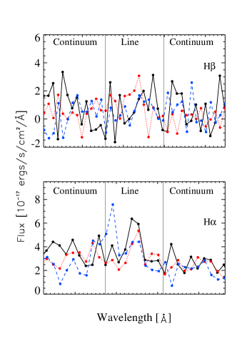
Figure 4: Three consecutive spectra (ordered by time: black/solid, red/dotted, blue/dashed) of an M5 star from the MSN sample that show no evidence of strong line flux in the H$\beta$ (top) and H$\alpha$ (bottom) line regions. The vertical lines mark the line regions used in the calculations. The EW values for the H$\beta$ are spuriously high in some exposures, while all of the FLI values are low. For the H$\alpha$ line, the FLI values are similar to the EW measurements. This demonstrates the usefulness of using FLI values when the continuum is weak or uncertain.

A commonly used measurement of emission line strength is the equivalent width (EW). However, EW measurements are problematic when the continuum flux near the line is weak and has low SNR. Figure 4 shows the H$\alpha$ and H$\beta$ line regions during a sequence of exposures of an M5 dwarf from our MSN sample. The H$\beta$ continuum flux is very close to zero, so division by the continuum to obtain EWs gives values of -3Å, 106Å, and 19Å  for the three consecutive exposures. While the star in Figure 4 is clearly not in a flaring state, the EW measurements for H$\beta$ are large and variable, as they might be during a flare. This issue could be avoided by limiting the sample to objects with high SNR in the H$\beta$ continuum (i.e., the HSN sample). However, including the MSN sample greatly increases our sample size. We therefore developed a new method for measuring line strength that is independent of the continuum strength. We define the Flare Line Index (FLI) as:

$$\mbox{FLI}=\bar{l}/\sigma,$$ (1)

where $\bar{l}$ is the mean value of the flux in the line region (for a specific emission line) minus the continuum flux (associated with the emission line; see Table 1) and $\sigma$ is the standard deviation of the continuum. The FLI measures the line strength in terms of its significance compared to the noise.

The FLI allows us to determine whether a line measurement is statistically significant even when the continuum is weak and/or uncertain. For the star in Figure 4, the FLI values for H$\beta$ are -0.3, 1.1, and 0.2, respectively. The differences in these values can be attributed to the noise in the spectra. The FLI values are neither as large nor as variable as the EW measurements of the same data. When the continuum is well-measured, as in the H$\alpha$ line, the FLI values and EW measurements are similar. The FLI does depend on the SNR of the spectra; stars with higher SNR have larger FLI values for the same emission line flux.

FLI values for both H$\alpha$ and H$\beta$ were computed for all spectra in the HSN and MSN samples and used in the subsequent analysis.

3.2 False Discovery Rate Analysis

Determining if an object is in a flaring state from a single spectrum is difficult because active stars have a range of nominal, non-flaring levels of H$\alpha$ activity. Also, there may be little difference between the emission line strengths of an active star in quiescence and those of a flaring star during a small flare or in the gradual phase of a large flare. We searched for flares based on the strength of the line emission, and on the variability in repeated spectral observations. We did not require that both criteria be met, since small flares may not have particularly strong lines, while large flares may not show much variability over the timescale of the SDSS observations.

We used False Discovery Rate (FDR; Miller et al., 2001) analysis to search for spectra with particularly strong emission lines that were outliers from the typical stellar distribution of FLI values. Our sample exhibits a continuous distribution of measured FLI values for both H$\alpha$ and H$\beta$, ranging from lines in absorption through emission and into the flare regime. FDR analysis is a quantitative method for determining a threshold value of a test statistic that separates real sources from a background (null) distribution for a given false-discovery rate. In our case, we sought to determine the FLI value above which stars were considered to be in a flaring state. The analysis uses an adaptive technique that establishes the threshold value based on the desired false positive rate, defined by the parameter $\alpha$. Our FDR method replaces an arbitrarily chosen confidence level (such as 3$\sigma$) with a known false positive rate and can select the outliers from our sample (as compared to the null) as flares while controlling the rate of false detections through the choice of $\alpha$. For our analysis, we limited the false positive rate to $\alpha=10\%$.

The key to using FDR analysis is to assemble a meaningful null distribution. In the case of identifying flares, the null distribution should be a set of spectra that have similar properties to our candidate flare sample, but contain no flares. Active M dwarf spectra (that are not flaring) will provide a good null sample for the flare analysis.

3.3 Constructing an Active Sample using FDR

The fraction of stars that are magnetically active increases from a few percent at spectral type M0 to nearly 100% at type M9 (Hawley et al., 1996; Gizis et al., 2000; West et al., 2004, 2008). Rather than simply adopting the active sample found by West et al. (2008), we tested the effectiveness of the FLI values and FDR analysis tools on our HSN and MSN samples by verifying that we could reproduce the West et al. (2008) results. Again, we require a null distribution to separate the active stars from the inactive ones. For this case, we adopted the DR5 composite spectra of inactive stars found by West et al. (2008) as the null distribution. We used the individual component spectra in the HSN and MSN samples as the test distribution. We carried out the analysis separately for each spectral type, although we found that the HSN sample only had sufficient numbers for the M0-3 types and the MSN sample for the M0-7 types (see Figure 3).

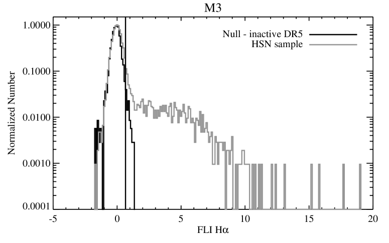
Figure 5: The distribution of FLI values for H$\alpha$ of the component spectra of M3 stars in the HSN sample (gray line) and the distribution of the null sample taken from the inactive DR5 integrated spectra (black line). The FDR-derived threshold value (vertical line) separates the inactive from the active and flaring spectra, which are seen as the high FLI value tail of the HSN sample.

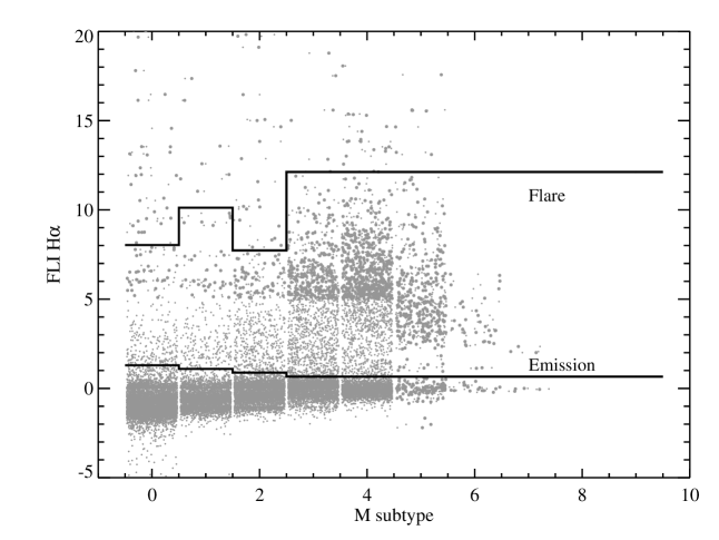
Figure 6: The H$\alpha$ FLI values from the HSN sample as a function of spectral subtype are shown as gray points. Each point has been given a random offset within its spectral type bin and enlarged where the point density is low for clarity. Most spectra have low FLI values, with the mean increasing with later spectral type, as expected from the activity fraction studies of West et al. (2004, 2006, 2008). The solid line labelled “Emission” indicates the FDR-derived threshold values separating active spectra from inactive ones, while the “Flare” line denotes the threshold values separating active stars from flares. Because our flare criteria require both H$\alpha$ and H$\beta$ to be above the relevant threshold value, not all points above the “Flare” line are categorized as flares in our sample.

An example of the FDR analysis for M3 stars is shown in Figure 5. The gray line represents the distribution of FLI values for the H$\alpha$ emission of the M3 dwarfs in the HSN sample (the test sample, which includes both active and inactive stars), while the black line represents the FLI distribution of the inactive M3 dwarfs from the DR5 composite spectra (the null sample, which contains only inactive stars). The distributions have been normalized to have the same peak value centered at FLI=0. The vertical line (at a FLI of 0.66) is the threshold value determined by the FDR analysis that divides active stars from inactive ones, with the false positive rate $\alpha$ set to 10%. The FLI emission threshold values we determined for the M0-3 spectral types in the HSN sample are shown in Figure 6 (labeled “Emission”). Note that for later types, the M3 value was adopted. Table 2 gives the H$\alpha$ FLI emission threshold values for both the HSN and MSN samples.

Using our FLI/FDR determination of activity, we found that 2.8% of the M0s are active and this fraction rises to 84% of M7-9 stars. These compare well to the active fractions reported by West et al. (2008), who found 2.6% and 90%, respectively. Although this agreement might be expected because we used the DR5 inactive spectra as our null distribution, we used a different test statistic (FLI instead of EW) and found our active sample using FDR analysis instead of defining an EW activity threshold of 1Å  on statistically significant emission lines in high SNR spectra (see West et al., 2004, for more details). The fact that we successfully recovered the same active stars gives us confidence that FLI values are a useful measure in cases where the EW is ill-defined, and that the FDR method can be used to distinguish between the distributions.

Table 2: FLI threshold values

	H$\alpha$						H$\beta$
	MSN			HSN			MSN		HSN
SpT	Emission	Flare		Emission	Flare		Flare		Flare
M0	1.12	2.97		1.29	8.03		0.61		3.44
M1	0.95	4.23		1.09	10.12		1.50		4.74
M2	0.96	7.76		0.88	7.73		2.20		7.43
M3	1.15	8.20		0.66	12.13		2.94		10.70
M4	0.76	9.73		…	…		6.12		…
M5	0.55	14.41		…	…		8.10		…
M6	0.68	10.80		…	…		7.52		…
M7	0.25	12.18		…	…		5.45		…

4 Flare Criteria

We used two separate methods to define whether or not an object in our sample contained a flare. The first was to use FDR analysis to determine which spectra had emission in both H$\alpha$ and H$\beta$ that was strong enough to be considered a flare. The other method was to find objects whose H$\alpha$ and H$\beta$ lines were both in emission and showed large variations together with time. These two methods are not mutually exclusive; flares that have strong emission lines that vary over the course of several exposures will meet both criteria.

4.1 Strong Emission Lines using FDR Analysis

We used the DR5 composite spectra of the active stars (i.e. those that met the emission threshold criteria determined from §3.3) as the null distribution for the flare FDR analysis.

Although the objects that make up the null distribution (the composite spectra) are the same objects that make up the test distribution (the individual exposures), the distributions are distinct in two significant ways. First, the signature of small flares that are only present in a subset of the exposures is diluted in the composite spectra. Second, outliers were removed from the null distribution by rejecting spectra that were not part of the continuous distribution of FLI values. A few small or diluted flares may still be present in the null distribution. However, any flares in the null will simply increase the threshold value determined in the analysis and decrease the number of objects classified as flares.

As in the active sample determination described in §3.3, we first normalized the null and test distributions, and then applied the FDR analysis separately to the HSN and MSN samples, for each M subtype. Again we found that the HSN sample analysis was limited to M0-3 types and the MSN sample to M0-7 types. The flare threshold values for both H$\alpha$ and H$\beta$ are given in Table 2, and are shown for the HSN sample in Figure 6. To be classified as a flare, we required that an individual spectrum had FLI values for both H$\alpha$ and H$\beta$ above the respective FDR flare threshold values. Thus, many of the spectra above the Flare line in Figure 6 were not found to be flares because they did not make the H$\beta$ cut. This effectively removed cases of H$\alpha$ activity that were not strong enough to be classified as flares.

4.2 Variable Emission Line Strength

We also identified flares by looking for variation in emission line strength among individual exposures of the same object. H$\alpha$ emission is known to vary outside of flaring (see discussion in §3); Gizis et al. (2002) and Lee et al. (2010) found that “quiescent” H$\alpha$ emission often varies by as much as 30% on short timescales (minutes-hours). This may well be due to low-level flaring, but it is not possible to classify unequivocally as flare emission due to the relatively poor time resolution of their data (and ours). We therefore concentrated on variability that exceeds this level (representing larger, definite flares), and developed the following flare criteria based on both the H$\alpha$ and H$\beta$ FLI values:

1. Mean FLI values $>$ 3 over all exposures for an object for both H$\alpha$ and H$\beta$; in these strong emission line spectra, we identified flares if both the H$\alpha$ and H$\beta$ FLI values for an object differed by more than 30% between the minimum and maximum values measured over the course of the exposures.

2. Mean FLI values $<$ 3 in both H$\alpha$ and H$\beta$; we identified flares in these weak emission line data using the criterion that max FLI - min FLI $>$ 3. We adopted an absolute change criterion because a 30% change is still within the noise when the mean FLI value is small. Since FLI is defined as $\bar{l}/\sigma$, this is essentially a 3$\sigma$ requirement (max FLI is 3$\sigma$ larger than min FLI).

3. Mean FLI values $>$ 3 in H$\alpha$ but $<$ 3 in H$\beta$; these objects have moderate emission strength in H$\alpha$ but weak emission in H$\beta$. We require that they meet both of the above variability criteria (max FLI - min FLI $>$ 3; percent change $>$ 30%) to be considered a flare.

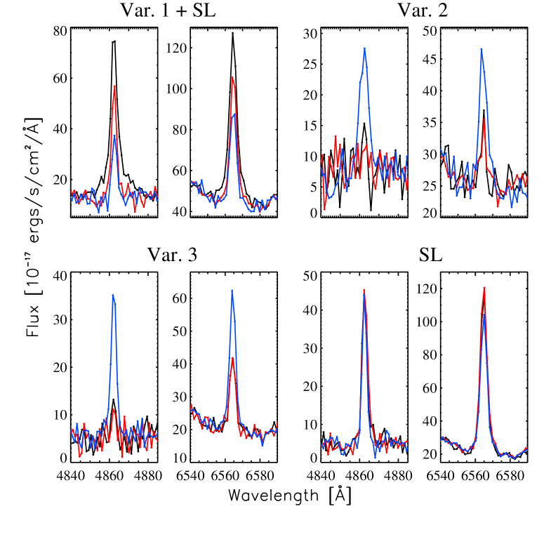
Figure 7: The H$\beta$ and H$\alpha$ lines of typical flares that meet each of the flare criteria (see §4.1 and 4.2 for details about the strong lines and variability criteria). Each panel shows all of the exposures for that object, with the black, red, and blue lines corresponding to the first, second, and third exposures, respectively. Note that the flare that meets the first variability criterion also meets the FDR strong lines criterion.

We examined objects that narrowly missed passing these flare criteria and confirmed that these quantitative measures are robust, and no real flares were omitted from the sample. Examples of flares that were identified based on each of these three conditions are shown in Figure 7. A large, decay-phase flare (top left) that met the first variability criterion (V1) also met the FDR strong lines criterion. The example flare that met the second variability criterion (V2, top right) demonstrated weak emission during the first two exposures, but had significantly stronger emission in the final exposure. The moderate quiescent emission example (bottom left) met the third variability criterion (V3) with a flare during the third exposure. The flare that met the FDR strong lines criterion (bottom right) showed very little change between exposures.

5 Results

Our automatic flare identification using the above methods resulted in 285 individual spectra on 72 M dwarfs being classified as flaring. We visually examined each spectrum and rejected 9 objects due to calibration errors, white dwarf companions, or cataclysmic variable signature. Our final flare sample therefore comprises 243 spectra on 63 stars. The properties of the 63 flaring stars are listed in Table 3.

Table 3: Properties of the flares in the SDSS Spectroscopic Sample

RA	Dec	SpT	Sample	# exp.	ID Method	Notes
40.71900	1.05628	M0	HSN	3	SL
355.34763	-0.64664	M1	HSN	5	V1
212.62507	38.67526	M2	HSN	3	SL
6.27294	0.26177	M3	MSN	3	SL
28.15489	0.94377	M3	HSN	3	SL + V1	rise
128.51469	23.71895	M3	HSN	3	V1
134.89224	28.22401	M3	HSN	3	V1
137.21883	25.20690	M3	HSN	3	SL + V1	decay
154.13328	36.06647	M3	HSN	3	V1
161.54023	42.75901	M3	HSN	6	V1	decay + quiet
179.32923	36.89933	M3	HSN	4	V1
231.35810	35.70936	M3	HSN	3	V1
246.65711	34.37560	M3	MSN	3	V2	has quiet
8.11627	-0.66997	M4	HSN	3	V1
13.71803	0.52899	M4	MSN	3	V3	has quiet
123.54478	7.83326	M4	HSN	4	V1
131.82185	3.01438	M4	HSN	8	V1	has quiet
138.47179	25.96210	M4	HSN	3	SL
138.91181	9.04170	M4	MSN	6	V3	has quiet
151.16178	39.81706	M4	HSN	3	V1	decay + quiet
178.31625	35.11017	M4	HSN	3	V1	rise
232.12920	38.05164	M4	MSN	4	SL
237.12605	51.50901	M4	HSN	3	V1	has quiet
238.82210	33.31065	M4	HSN	3	V1
358.33475	0.27060	M4	MSN	3	SL + V1	decay
24.02448	-1.12992	M5	MSN	5	SL + V1	has quiet
114.81201	31.09497	M5	MSN	3	V3	rise + quiet
115.68026	35.39034	M5	MSN	12	V3	has quiet
116.05362	41.68687	M5	MSN	8	V3	decay + quiet
116.72870	36.04137	M5	HSN	12	V1
123.96988	32.28493	M5	MSN	3	V3	rise + quiet
129.77425	6.91552	M5	MSN	4	V3	peak
136.04183	42.06829	M5	MSN	4	V1
136.09474	0.26750	M5	MSN	3	SL
156.27249	57.84446	M5	MSN	3	V2	has quiet
163.10690	37.36536	M5	HSN	3	V1	rise
181.06226	32.77287	M5	HSN	3	SL + V1	rise + quiet
196.07931	15.21429	M5	MSN	3	V1	decay
208.73389	48.89529	M5	MSN	4	V1
211.05023	4.04835	M5	MSN	3	V3	peak
213.01983	54.68985	M5	MSN	3	V1	has quiet
217.63041	57.17282	M5	HSN	3	V1
219.60447	39.63877	M5	MSN	4	V3	rise + quiet
225.05331	60.90313	M5	MSN	3	V1	peak
248.08604	23.94904	M5	HSN	3	V1	rise
3.28885	-0.43108	M6	MSN	3	SL + V1
53.72138	-7.31779	M6	MSN	3	SL + V1	cont. emission
118.05603	27.77888	M6	MSN	4	V2	rise + quiet
130.79823	35.31980	M6	MSN	3	V1	decay
143.62620	3.87247	M6	MSN	6	V3	decay
148.58678	34.44622	M6	MSN	3	V1
194.47690	3.55015	M6	MSN	3	SL + V1	cont. emission
195.65088	6.03001	M6	MSN	4	SL + V1	decay
240.34528	51.89663	M6	MSN	3	V1	peak
240.91342	38.51986	M6	MSN	3	SL
329.51701	-8.35545	M6	MSN	3	V3	has quiet
119.29499	42.94881	M7	MSN	4	SL
135.52879	0.55538	M7	MSN	4	V1	peak
180.38979	40.77934	M7	MSN	4	SL + V1	rise
193.30205	40.56684	M7	MSN	3	SL	decay
234.07976	33.08753	M7	MSN	3	SL + V1	decay
30.09824	0.64641	M8	MSN	3	SL
182.07041	8.75788	M9	MSN	4	SL + V3	has quiet

A summary of the number of stars and exposures that met each flare criterion is presented in Table 4, which also shows that the majority of flares come from the MSN sample. This is not unexpected, since there are many more stars in that sample. Our results suggest that flares in this sparsely sampled spectroscopic data set are most easily identified through emission line variability rather than the absolute strength of the emission lines.

Table 4: Flare identification by emission line strength and variability criteria

	SL			V1			V2			V3			SL + V1			SL + V3
	Stars	Exp.		Stars	Exp.		Stars	Exp.		Stars	Exp.		Stars	Exp.		Stars	Exp.
HSN	3	9		18	75		0	0		0	0		3	9		0	0
MSN	7	23		9	30		3	10		11	55		8	28		1	4
Total	10	32		27	105		3	10		11	55		11	37		1	4

5.1 Time Evolution of Flares

We first analyzed our flare sample to verify that the properties of the flares we identified are consistent with the characteristic time evolution seen in continuous monitoring observations. Because our data might capture any or all phases of a flare, we expected to see examples of flares in the rise, peak, and decay phases as well as a few large impulsive phase flares that show blue continuum flux enhancement.

5.1.1 Rise, Peak, and Decay Phase Flares

We defined decay-phase flares as those showing both H$\alpha$ and H$\beta$ in at least two consecutive exposures with diminishing FLI values. Rise-phase flares were defined in the opposite sense, with two or more consecutive exposures having increasing FLI values for both H$\alpha$ and H$\beta$. There were ten rise phase flares and 11 decay phase flares in the sample. Additionally, we saw five “peak” flares that show first increasing and then decreasing FLI values, which we interpret as flares that were seen through most of their evolution. We also identified flares that occurred in only a subset of the exposures, either in the final exposure of a sequence, or in cases where some of the exposures are separated by many hours or days from the other exposures. In 19 cases, at least one exposure was obtained that showed a quiescent spectrum with no sign of flaring. Flares with quiescent spectrum, as well as rise, decay, and peak phase flares are noted in the final column of Table 3. The time evolution of the flares we have identified is consistent with the known characteristics of flares.

5.1.2 The Balmer decrements of Rise and Decay Flares

Previous observations using time resolved spectroscopic monitoring have shown that the higher order Balmer lines show larger increases in flux during flares than the lower order lines. This results in the observed Balmer decrement (ratio of individual lines to a fiducial, often H$\beta$ as we adopt here) becoming flatter, since H$\gamma$ and the higher order lines strengthen relative to H$\beta$ (García-Alvarez et al., 2002; Allred et al., 2006, see also Figure 7 of Bochanski et al. 2007) This behavior can be explained by a model where flare heating increases the local electron density at chromospheric temperatures. The higher order Balmer lines are less optically thick than the lower order lines, so the increase in electron density causes a relatively larger increase in their emission. The H$\alpha$ line behavior relative to the other lines has previously been more difficult to measure during flares, since observations typically concentrated on the blue part of the spectrum (e.g. Hawley & Pettersen, 1991). Along with their blue spectra, (Eason et al., 1992) obtained data with a different instrument at lower time resolution showing that the H$\alpha$ line, being already very optically thick, does not respond strongly during a large flare in accord with models (Allred et al., 2006).

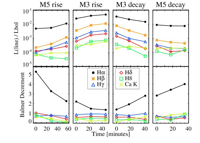
Figure 8: Line fluxes of emission lines normalized by the bolometric luminosity for two rise phase flares and two decay phase flares (top). Note that Ca II K (crosses) does not follow the same trend as the Balmer lines. The bottom panels show the Balmer decrements for the same flares. The H$\alpha$ decrement is smaller when the flare is closer to its peak (later for rise phase flares, and earlier for decay phase flares).

Figure 8 illustrates the line flux normalized to the bolometric luminosity for several lines (top), as well as Balmer decrements for four flares (bottom; two rise- and two decay-phase). The Balmer lines increase during the rise phase flares, and decrease during the decay phase flares, as expected. In the bottom panels, we see that for all of the Balmer lines except H$\alpha$, the decrements are flat throughout the flares. As expected, the H$\alpha$ decrement decreases during the rise-phase, when H$\beta$ is becoming relatively stronger, and increases during the decay-phase, as the atmosphere gradually returns to its quiescent temperature and density structure. Our observations are in accord with expectations, and actually represent truly simultaneous measurements with the same instrument of the entire Balmer decrement (including H$\alpha$) during stellar flares.

The Ca II K line responds less strongly, and rises and decays more slowly during flares, than the Balmer lines (Butler, 1991; Hawley & Pettersen, 1991), as is also evident from our observations.

5.1.3 Continuum Flux Enhancement

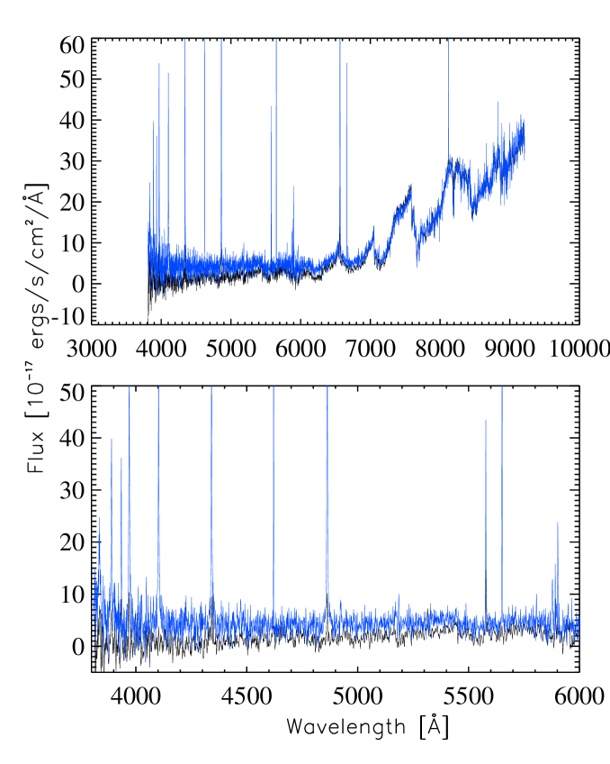
Figure 9: The spectrum of an M6 dwarf (R.A., Dec. = 194.47690, 3.55015) during quiescence (black) and during a flare (blue). This exposure captures at least part of the impulsive phase of the flare and shows a clear continuum enhancement in the blue portion of the spectrum (shown in the bottom panel), as well as strong emission lines.

Large flares cause strong blue continuum flux enhancement, with less dramatic effects at redder wavelengths. Only very strong flares caught in the impulsive phase would lead to a significant flux enhancement for the wavelength range and relatively long exposure times (which dilute the short-lived continuum burst) of the SDSS spectra. We expected to find only a small number of such flares, since large flares are rare and we are only sensitive to measuring continuum enhancement on HSN stars or very bright MSN stars, where we have a good measure of the quiescent continuum. Our sample contained two continuum flares, an example of which is shown in Figure 9. Both flares occurred during the third and final exposure of a series, and both show very strong emission lines. These are evidently large flares that were caught during the impulsive phase. We measured the flare-only spectrum by subtracting the quiescent (first) exposure obtained for each star from the flare exposure. We found that the continuum flux represented 88% and 90% of the total flare radiation, respectively, with the remainder of the energy coming from the line radiation. Hawley & Pettersen (1991) found that the continuum emitted 96% of the flare flux during the impulsive phase of their very large flare, and averaged 91% over the course of the flare. This suggests that our flare exposures may have included the impulsive phase and part of the decay phase of each flare. The existence of these continuum flare spectra in our sample, and the relative strength of the lines and continua, give us additional confidence that we are correctly identifying flares by our automatic algorithms.

5.2 Flare Duty Cycle

Figure 10 shows our observed flare duty cycle as a function of spectral type. The duty cycle increases with later spectral type, from 0.02% for M0 stars to 20% for M9 stars. The error bars were calculated from binomial statistics, and the number of flares identified at each spectral type is noted. The numbers in parentheses are the number of flares identified by the variability criteria. The much larger duty cycles for M7 and later are based on a small number of stars, and although there are many thousands of objects in the M0-M3 bins, there are very few flares. In order to improve the statistics, we binned by spectral type and found the duty cycles to be $0.022\pm 0.016\%$ of M0-1 stars; $0.077\pm 0.023\%$ for M2-3 stars; $0.56\pm 0.09\%$ for M4-6 stars; and $3\pm 1\%$ of M7-9 stars.

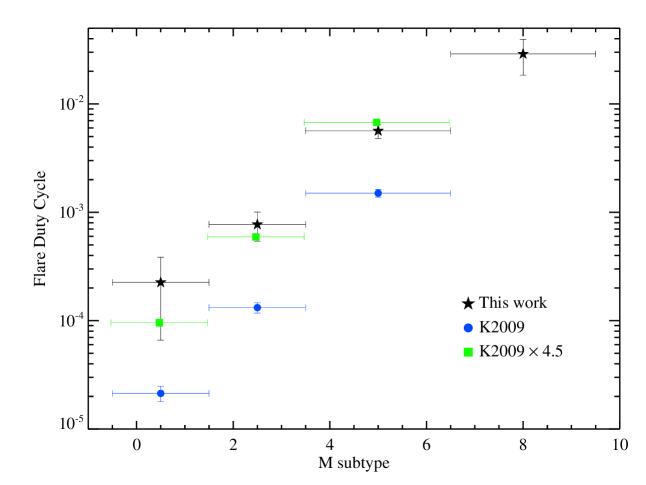
Figure 11: The flare duty cycle as measured by Kowalski et al. (2009, closed circles) and this study (stars), for spectral type bins M0-1, M2-3, M4-6, M7-9. Scaling the Kowalski et al. (2009) results by a factor of 4.5 (squares) makes them consistent with our results.

Kowalski et al. (2009) investigated flares in a large SDSS photometric sample. They required near simultaneous photometric enhancements in both the $u$ and $g$ filters, and employed a threshold of $|\Delta u|>$ 0.7 to define a flare. Figure 11 compares their flare duty cycle with our results for the binned data. We find a higher duty cycle, by a factor of $\sim$ 4.5, but the duty cycle as a function of spectral type has a similar trend in both studies. It is not surprising that the duty cycles are different, since the two studies use such different observations and threshold criteria. However, we can qualitatively estimate the effect of observing line versus continuum enhancements, and the effect of exposure time. The line emission remains enhanced for much longer than the continuum emission leading to a higher probability of observing flares in line emission. Longer exposure times increase the chance of a flare occurring during the exposure. Both of these factors lead to the observed higher duty cycle seen in our spectroscopic observations.

5.3 The Vertical Distribution of Flaring Stars in the Galaxy

Nearly all flares occur on magnetically active stars, as defined by H$\alpha$ in emission (Reid et al., 1999; Kowalski et al., 2009). As discussed in Section 3.3, the active fraction increases with spectral subtype. In addition, West et al. (2008) found that the active fraction decreases with vertical height from the Galactic Plane (denoted by $|$Z$|$) for all spectral types, which they attribute to an age effect, where older stars are less likely to be active. The age at which activity disappears changes with spectral type however, with later type M dwarfs remaining active for a longer time.

We limited our analysis of the vertical distribution of the flaring stars to just the M4-6 dwarfs, which show a large number of flares, and have a similar flaring fraction (see Figure 10). Earlier type stars have very few flares, and later type stars are too faint to be observed at large distances.

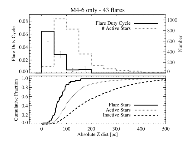
Figure 12: Top: The flare duty cycle as a function of distance from the Galactic midplane ($|$Z$|$) for M4-6 stars (black line). The number of active stars (West et al., 2008) in the sample is also shown (gray line, dotted, right axis). The fraction of objects that flare decreases rapidly with distance from the Galactic Plane. Bottom: the cumulative distribution of absolute Z distance for the flare, active, and inactive stars between subtype M4 and M6. These results indicate that flaring occurs preferentially closer to the Galactic Plane than the general active star population, and therefore on younger stars.

Figure 12 (top panel) shows the distribution of active M4-6 dwarfs and the fraction that showed flares as a function of vertical distance from the Galactic Plane. We repeated our analysis, adjusting both the bin size and bin positions and verified that the increase in flare fraction as a function of $|$Z$|$ is a real effect and not an artifact of the binning process. The bottom panel of Figure 12 shows the cumulative distributions of the flare stars (black line), the active stars (dotted gray line) and the inactive stars (dashed line). Although there are thousands of objects beyond $|$Z$|$=200 pc, none of them showed flares. Kowalski et al. (2009) and Welsh et al. (2007) also found that all of the flares on M4 dwarfs occur within 200pc of the Plane.

Our results indicate that flares occur on stars that are preferentially closer to the Plane than the inactive stars, and closer even than the active population. If we interpret this in terms of an age effect, it suggests that flare stars (which are a subset of the active population) are younger than the magnetically active stars as a whole. Evidently the frequency of flaring decreases as a star ages, although it still may exhibit quiescent chromospheric emission and therefore be counted as active.

6 Conclusion

We have presented the first study to systematically search for flares in a sample of tens of thousands of time-resolved spectroscopic observations from the SDSS Data Release 6. We developed two new techniques for identifying and analyzing flares in relatively low SNR spectra: the Flare Line Index (FLI) measurement and the application of the False Discovery Rate to flare spectra. FLI values provide a measure of emission line strength even when the continuum level is not well-measured. The FDR analysis distinguishes between the overlapping distributions in line strength of strong quiescent emission and genuine flares, providing a threshold FLI value for being considered a flare, while controlling the rate of false-positives. Using our measured FLI values for the H$\alpha$ and H$\beta$ lines, we applied the FDR analysis and a set of variability criteria to find flares.

We identified flares on 63 stars from the 30,971 total stars comprising both the HSN and MSN samples. The flares include examples of rise and decay phases, as well as some sequences of exposures that appear to trace the flare through its entire evolution. The Balmer decrements are consistent with results from time resolved spectroscopic monitoring of individual flares and expectations of models. We also found two flares that show continuum flux enhancements, which occur during the initial impulsive phase of large flares. Because the properties of the flares in our sample are consistent with previous findings, we are confident that our techniques, which we developed specifically to work with coarsely time-resolved spectroscopic observations, successfully identified flares.

We found that the flare duty cycle increases monotonically as a function of M dwarf spectral subtype, from $0.022\pm 0.016\%$ of M0-1 stars to $3\pm 1\%$ of M7-9 stars. The flare distribution as a function of spectral subtype is similar to the distribution of active stars, providing further evidence that most flares occur on active stars. Nearly all of the flares in the sample occur on stars near the Galactic Plane, a result that is consistent with other studies (i.e. Kowalski et al., 2009). Furthermore, we have shown that flares occur preferentially on stars closer to the Plane than the mean active population, indicating that flare frequency likely decreases with age.

This study represents an important step toward understanding the intrinsic flare frequency distribution as a function of stellar active lifetimes. Surveys that don’t have high time resolution and continuous coverage (from which the total flare energy can be computed) require detailed and nuanced Monte Carlo simulations in order to constrain the physical flare frequency distribution. Simulations which consider stellar samples in the Galactic context is the subject of ongoing study (Hilton et al., in prep).

The authors would like to thank J. Wisniewski, S. Schmidt, and J. Davenport for fruitful discussions that improved this paper. They would also like to thank D. Schlegel for assistance in obtaining the data. E.J.H., S.L.H. and A.F.K acknowledge support from NSF grant AST 08-07205.

Funding for the SDSS and SDSS-II has been provided by the Alfred P. Sloan Foundation, the Participating Institutions, the National Science Foundation, the U.S. Department of Energy, the National Aeronautics and Space Administration, the Japanese Monbukagakusho, the Max Planck Society, and the Higher Education Funding Council for England. The SDSS Web site is http://www.sdss.org/. The SDSS is managed by the Astrophysical Research Consortium for the Participating Institutions. The Participating Institutions are the American Museum of Natural History, Astrophysical Institute Potsdam, University of Basel, University of Cambridge, Case Western Reserve University, University of Chicago, Drexel University, Fermilab, the Institute for Advanced Study, the Japan Participation Group, Johns Hopkins University, the Joint Institute for Nuclear Astrophysics, the Kavli Institute for Particle Astrophysics and Cosmology, the Korean Scientist Group, the Chinese Academy of Sciences (LAMOST), Los Alamos National Laboratory, theMax-Planck- Institute for Astronomy (MPIA), the Max-Planck-Institute for Astrophysics (MPA), New Mexico State University, Ohio State University, University of Pittsburgh, University of Portsmouth, Princeton University, the United States Naval Observatory, and the University of Washington.

Figure 1: Histograms of the exposure times for all component spectra in the sample (left) and of the exposure times for the component spectra (right). The dashed histograms are for the entire West et al. (2008) sample, while the solid histograms are the stars considered in this study.

Figure 3: The distribution of spectral subtypes for the HSN (dotted), MSN (dashed), and total (solid) samples. As expected, the HSN sample mostly contains the earlier, and intrinsically brighter, spectral subtypes. Although the MSN sample has more later spectral subtype stars, there are relatively few beyond M6.

Figure 10: The flare duty cycle as a function of spectral type. The error bars are calculated from the binomial distribution. The number of flares in each bin is given, with the number of flares that meet the variability criteria given in parentheses. The flare fraction increases with spectral subtype as expected from previous studies, and is similar to the rise in the active fraction of M dwarfs.

References

- Adelman-McCarthy et al. (2008) Adelman-McCarthy, J. K., et al. 2008, ApJS, 175, 297
- Adelman-McCarthy et al. (2007) —. 2007, ApJS, 172, 634
- Allred et al. (2006) Allred, J. C., Hawley, S. L., Abbett, W. P., & Carlsson, M. 2006, ApJ, 644, 484
- Audard et al. (2000) Audard, M., Güdel, M., Drake, J. J., & Kashyap, V. L. 2000, ApJ, 541, 396
- Berger et al. (2008) Berger, E., et al. 2008, ApJ, 673, 1080
- Bochanski et al. (2007) Bochanski, J. J., West, A. A., Hawley, S. L., & Covey, K. R. 2007, AJ, 133, 531
- Bopp & Schmitz (1978) Bopp, B. W., & Schmitz, M. 1978, PASP, 90, 531
- Butler (1991) Butler, C. J. 1991, Memorie della Societa Astronomica Italiana, 62, 243
- Charbonneau et al. (2009) Charbonneau, D., et al. 2009, Nature, 462, 891
- Cincunegui et al. (2007) Cincunegui, C., Díaz, R. F., & Mauas, P. J. D. 2007, A&A, 469, 309
- Correia et al. (2010) Correia, A. C. M., et al. 2010, A&A, 511, A21+
- Covey et al. (2007) Covey, K. R., et al. 2007, AJ, 134, 2398
- Crespo-Chacón et al. (2006) Crespo-Chacón, I., Montes, D., García-Alvarez, D., Fernández-Figueroa, M. J., López-Santiago, J., & Foing, B. H. 2006, A&A, 452, 987
- Eason et al. (1992) Eason, E. L. E., Giampapa, M. S., Radick, R. R., Worden, S. P., & Hege, E. K. 1992, AJ, 104, 1161
- Forveille et al. (2009) Forveille, T., et al. 2009, A&A, 493, 645
- Fuhrmeister et al. (2007) Fuhrmeister, B., Liefke, C., & Schmitt, J. H. M. M. 2007, A&A, 468, 221
- Fuhrmeister & Schmitt (2004) Fuhrmeister, B., & Schmitt, J. H. M. M. 2004, A&A, 420, 1079
- García-Alvarez et al. (2002) García-Alvarez, D., Jevremović, D., Doyle, J. G., & Butler, C. J. 2002, A&A, 383, 548
- Gershberg & Shakhovskaia (1983) Gershberg, R. E., & Shakhovskaia, N. I. 1983, Ap&SS, 95, 235
- Gizis et al. (2000) Gizis, J. E., Monet, D. G., Reid, I. N., Kirkpatrick, J. D., Liebert, J., & Williams, R. J. 2000, AJ, 120, 1085
- Gizis et al. (2002) Gizis, J. E., Reid, I. N., & Hawley, S. L. 2002, AJ, 123, 3356
- Haisch et al. (1991) Haisch, B., Strong, K. T., & Rodono, M. 1991, ARA&A, 29, 275
- Hawley et al. (2003) Hawley, S. L., et al. 2003, ApJ, 597, 535
- Hawley et al. (1995) —. 1995, ApJ, 453, 464
- Hawley et al. (1996) Hawley, S. L., Gizis, J. E., & Reid, I. N. 1996, AJ, 112, 2799
- Hawley & Pettersen (1991) Hawley, S. L., & Pettersen, B. R. 1991, ApJ, 378, 725
- Heath et al. (1999) Heath, M. J., Doyle, L. R., Joshi, M. M., & Haberle, R. M. 1999, Origins of Life and Evolution of the Biosphere, 29, 405
- Kaiser (2004) Kaiser, N. 2004, in Presented at the Society of Photo-Optical Instrumentation Engineers (SPIE) Conference, Vol. 5489, Ground-based Telescopes. Edited by Oschmann, Jacobus M., Jr. Proceedings of the SPIE, Volume 5489, pp. 11-22 (2004)., ed. J. M. Oschmann, Jr., 11–22
- Kowalski et al. (2009) Kowalski, A. F., Hawley, S. L., Hilton, E. J., Becker, A. C., West, A. A., Bochanski, J. J., & Sesar, B. 2009, AJ, 138, 633
- Kowalski et al. (2010) Kowalski, A. F., Hawley, S. L., Holtzman, J. A., Wisniewski, J. P., & Hilton, E. J. 2010, ApJ, 714, L98
- Lacy et al. (1976) Lacy, C. H., Moffett, T. J., & Evans, D. S. 1976, ApJS, 30, 85
- Lee et al. (2010) Lee, K., Berger, E., & Knapp, G. R. 2010, ApJ, 708, 1482
- Leto et al. (1997) Leto, G., Pagano, I., Buemi, C. S., & Rodono, M. 1997, A&A, 327, 1114
- LSST Science Collaborations: Paul A. Abell et al. (2009) LSST Science Collaborations: Paul A. Abell, et al. 2009, ArXiv e-prints
- Martín & Ardila (2001) Martín, E. L., & Ardila, D. R. 2001, AJ, 121, 2758
- Mayor et al. (2009) Mayor, M., et al. 2009, A&A, 507, 487
- Miller et al. (2001) Miller, C. J., et al. 2001, AJ, 122, 3492
- Moffett (1974) Moffett, T. J. 1974, ApJS, 29, 1
- Osten et al. (2005) Osten, R. A., Hawley, S. L., Allred, J. C., Johns-Krull, C. M., & Roark, C. 2005, ApJ, 621, 398
- Pettersen et al. (1984) Pettersen, B. R., Coleman, L. A., & Evans, D. S. 1984, ApJS, 54, 375
- Rau et al. (2009) Rau, A., et al. 2009, PASP, 121, 1334
- Reid et al. (1999) Reid, I. N., Kirkpatrick, J. D., Gizis, J. E., & Liebert, J. 1999, ApJ, 527, L105
- Robinson et al. (1999) Robinson, R. D., Carpenter, K. G., & Percival, J. W. 1999, ApJ, 516, 916
- Robinson et al. (1995) Robinson, R. D., Carpenter, K. G., Percival, J. W., & Bookbinder, J. A. 1995, ApJ, 451, 795
- Sanz-Forcada & Micela (2002) Sanz-Forcada, J., & Micela, G. 2002, A&A, 394, 653
- Schmidt et al. (2007) Schmidt, S. J., Cruz, K. L., Bongiorno, B. J., Liebert, J., & Reid, I. N. 2007, AJ, 133, 2258
- Segura et al. (2005) Segura, A., Kasting, J. F., Meadows, V., Cohen, M., Scalo, J., Crisp, D., Butler, R. A. H., & Tinetti, G. 2005, Astrobiology, 5, 706
- Segura et al. (2010) Segura, A., Walkowicz, L., Meadows, V., Kasting, J., & Hawley, S. 2010, ArXiv e-prints
- Smolčić et al. (2004) Smolčić, V., et al. 2004, ApJ, 615, L141
- Tarter et al. (2007) Tarter, J. C., et al. 2007, Astrobiology, 7, 30
- Udry et al. (2007) Udry, S., et al. 2007, A&A, 469, L43
- Walker (1981) Walker, A. R. 1981, MNRAS, 195, 1029
- Walkowicz & Hawley (2009) Walkowicz, L. M., & Hawley, S. L. 2009, AJ, 137, 3297
- Walkowicz et al. (2008) Walkowicz, L. M., Johns-Krull, C. M., & Hawley, S. L. 2008, ApJ, 677, 593
- Welsh et al. (2007) Welsh, B. Y., et al. 2007, ApJS, 173, 673
- West et al. (2006) West, A. A., Bochanski, J. J., Hawley, S. L., Cruz, K. L., Covey, K. R., Silvestri, N. M., Reid, I. N., & Liebert, J. 2006, AJ, 132, 2507
- West et al. (2008) West, A. A., Hawley, S. L., Bochanski, J. J., Covey, K. R., Reid, I. N., Dhital, S., Hilton, E. J., & Masuda, M. 2008, AJ, 135, 785
- West et al. (2004) West, A. A., et al. 2004, AJ, 128, 426
- Zhilyaev et al. (2007) Zhilyaev, B. E., et al. 2007, A&A, 465, 235