Non-linear QCD dynamics in two-photon interactions at high energies

Abstract

Perturbative QCD predicts that the growth of the gluon density at high energies should saturate, forming a Color Glass Condensate (CGC), which is described in mean field approximation by the Balitsky-Kovchegov (BK) equation. In this paper we study the $\gamma\gamma$ interactions at high energies and estimate the main observables which will be probed at future linear colliders using the color dipole picture. We discuss in detail the dipole - dipole cross section and propose a new relation between this quantity and the dipole scattering amplitude. The total $\gamma\gamma$, $\gamma^{*}\gamma^{*}$ cross-sections and the real photon structure function $F_{2}^{\gamma}(x,Q^{2})$ are calculated using the recent solution of the BK equation with running coupling constant and the predictions are compared with those obtained using phenomenological models for the dipole-dipole cross section and scattering amplitude. We demonstrate that these models are able to describe the LEP data at high energies, but predict a very different behavior for the observables at higher energies. Therefore we conclude that the study of $\gamma\gamma$ interactions can be useful to constrain the QCD dynamics.

I Introduction

The high energy limit of perturbative QCD is characterized by a center-of-mass energy which is much larger than the hard scales present in the problem. The simplest process where this limit can be studied is the high energy scattering between two heavy quark-antiquark states, i.e. the onium-onium scattering. For a sufficiently heavy onium state, high energy scattering is a perturbative process since the onium radius gives the essential scale at which the running coupling $\alpha_{s}$ is evaluated. In the dipole picture dipole , the heavy quark-antiquark pair and the soft gluons in the limit of large number of colors $N_{c}$ are viewed as a collection of color dipoles. In this case, the cross section can be understood as a product of the number of dipoles in one onium state, the number of dipoles in the other onium state and the basic cross section for dipole-dipole scattering. At leading order (LO), the cross section grows rapidly with the energy ($\sigma\propto\alpha_{s}^{2}\,e^{(\alpha_{{I\!\!P}}-1)Y}$, where $(\alpha_{{I\!\!P}}-1)=\frac{4\alpha_{s}\,N_{c}}{\pi}\,\ln 2\approx 0.5$ and $Y=\ln\,s/Q^{2}$) because the LO BFKL equation bfkl predicts that the number of dipoles in the light cone wave function grows rapidly with the energy. Several shortcomings are present in this calculation. Firstly, in the leading order calculation the energy scale is arbitrary, which implies that the absolute value of the total cross section is therefore not predictable. Secondly, $\alpha_{s}$ is not running at LO BFKL. Finally, the power growth with energy violates $s$-channel unitarity at large energies. Consequently, new physical effects should modify the LO BFKL equation at very large $s$, making the resulting amplitude unitary.

A theoretical possibility to modify this behavior in a way consistent with the unitarity is the idea of parton saturation, where non-linear effects associated to high parton density are taken into account. The basic idea is that when the parton density increases (and the scattering amplitude tends to the unitarity limit), the linear description present in the BFKL equation breaks down and one enters the saturation regime. In this regime, the growth of the parton distribution is expected to saturate, forming a Color Glass Condensate (CGC), whose evolution with energy is described by an infinite hierarchy of coupled equations for the correlators of Wilson lines (For recent reviews see cgc ). In the mean field approximation, the first equation of this hierarchy decouples and boils down to a single non-linear integro-differential equation: the Balitsky-Kovchegov (BK) equation. In the last years the next-to-leading order corrections to the BK equation were calculated kovwei1 ; javier_kov ; balnlo through the ressumation of $\alpha_{s}N_{f}$ contributions to all orders, where $N_{f}$ is the number of flavors. Such calculation allows one to estimate the soft gluon emission and running coupling corrections to the evolution kernel. The authors have found that the dominant contributions come from the running coupling corrections, which allow us to determine the scale of the running coupling in the kernel. The solution of the improved BK equation was studied in detail in Ref. javier_kov . In bkrunning a global analysis of the small $x$ data for the proton structure function using the improved BK equation was performed (See also Ref. weigert ). In contrast to the BK equation at leading logarithmic $\alpha_{s}\ln(1/x)$ approximation, which fails to describe the HERA data, the inclusion of running coupling effects in the evolution renders the BK equation compatible with them (See also vic_joao ; alba_marquet ; vicmagane ).

A reaction which is analogous to the process of scattering of two onia discussed above is the off-shell photon scattering at high energy in $e^{+}\,e^{-}$ colliders, where the photons are produced from the lepton beams by bremsstrahlung (For a review see, e.g., Ref. nisius ). In these two-photon reactions, the photon virtualities can be made large enough to ensure the applicability of perturbative methods or can be varied in order to test the transition between the soft and hard regimes of the QCD dynamics. From the point of view of the BFKL approach, there are several calculations using the leading logarithmic approximation bartels ; gamboone and considering some of the next-to-leading corrections to the total $\gamma^{*}\gamma^{*}$ cross section gamboone ; gammaNLO ; victor_sauter ; papa . On the other hand, the successful description of all inclusive and diffractive deep inelastic data from HERA by saturation models GBW ; bgbk ; kw ; kmw ; fss04 ; fss06 ; kkt ; iim ; dhj ; gkmn ; mps07 ; marquet07 ; buw ; soyez ; watt08 suggests that these effects might become important in the energy regime probed by current colliders. This motivated the generalization of the saturation model to two-photon interactions at high energies performed in Ref. Kwien_Motyka , which has obtained a very good description of the data on the $\gamma\gamma$ total cross section, on the photon structure function at low $x$ and on the $\gamma^{*}\gamma^{*}$ cross section. The formalism used in Ref. Kwien_Motyka is based on the dipole picture dipole , with the $\gamma^{*}\gamma^{*}$ total cross sections being described by the interaction of two color dipoles, in which the virtual photons fluctuate into (For previous analysis using the dipole picture see, e.g., Refs. nik_photon ; dona_dosch ). The main assumption made in Kwien_Motyka is that the dipole-dipole cross section can be expressed in terms of dipole-proton cross section with the help of the additive quark model. This is a strong assumption which deserves a more detailed analysis. This is our first goal in this paper. In particular, we propose a more sophisticated connection between the dipole - dipole and dipole - proton scattering amplitudes. Our second goal is to compare the predictions obtained using Kwien_Motyka with those obtained with our approach. We also discuss the dependence of the results on the dipole scattering amplitude. Here we make use of the state-of-the art parametrization of the dipole scattering amplitude bkrunning . We compare the results with the currently available experimental data and provide estimates of the total cross sections and photon structure functions which will be measured in the future linear colliders. It is important to emphasize that in Kwien_Motyka the cross sections were estimated considering the GBW model GBW , which is inspired on saturation physics, and during the last years an intense activity in the area resulted in more sophisticated dipole - proton cross sections bgbk ; kw ; kmw ; fss04 ; fss06 ; kkt ; iim ; dhj ; gkmn ; mps07 ; marquet07 ; buw ; soyez ; watt08 , which could be used to estimate the $\gamma\gamma$ cross sections. In our study we also compare the predictions obtained using the solution of the BK equation with those from the phenomenological saturation model proposed in iim with free parameters updated in soyez .

Before introducing the required formulas, some comments are in order. Firstly, in our study the heavy quark contribution is not included, since the solution of the BK equation used in our calculations bkrunning has its free parameters fixed disregarding the contribution of heavy quarks to the inclusive and longitudinal structure functions. Recently, this solution was improved by including the charm and bottom contributions to these observables, which have strong effects on the fit parameters aamqs . As this solution is not yet public, we postpone for a future study the discussion of heavy quark production in $\gamma\gamma$ interactions. For consistence we also consider the phenomenological saturation model proposed in iim without the inclusion of heavy quarks. However, we also consider the updated version obtained in soyez , where the free parameters were fixed considering the more recent H1 and ZEUS data. Secondly, we are assuming in our study that fluctuations and correlations produced by the BK equation in the dilute regime (see, for instance, Refs. pom_loop ), where this equation reduces to the BFKL equation, can be neglected in the calculation of the dipole - dipole scattering cross section. This is a strong assumption. However, results obtained using a toy model in portugal , indicate that these effects are tamed by saturation in the high-density regime and by the running of coupling in the dilute regime. As in our model the scattering amplitude is given in terms of the solution of the BK equation including running coupling corrections, we expect the contribution of fluctuations to be small.

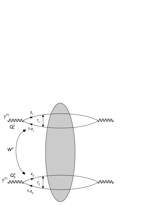
Figure 1: The diagram illustrating the $\gamma^{*}\gamma^{*}$ interaction in the dipole representation. See formula (1).

II The dipole picture for the two-photon cross section

Let us start presenting a brief review of the two-photon interactions in the dipole picture. At high energies, the scattering process can be seen as a succession in time of two factorizable subprocesses (See Fig. 1): i) the photon fluctuates into quark-antiquark pairs (the dipoles), ii) these color dipoles interact and produce the final state. The corresponding cross section is given by

$$\sigma_{ij}(W^{2},Q_{1}^{2},Q_{2}^{2})\;=\;\sum_{a,b=1}^{N_{f}}\int dz_{1}\int d^{2}\mbox{\boldmath$r$}_{1}\,|\Psi_{i}^{a}(z_{1},{\mbox{\boldmath$r$}_{1}})|^{2}\int dz_{2}\int d^{2}\mbox{\boldmath$r$}_{2}\,|\Psi_{j}^{b}(z_{2},{\mbox{\boldmath$r$}_{2}})|^{2}\;\sigma^{dd}_{a,b}(\mbox{\boldmath$r$}_{1},\mbox{\boldmath$r$}_{2},Y),$$ (1)

where $W^{2}$ is the collision center of mass energy squared, the indices $i,j$ label the polarisation states of the virtual photons, i.e. $T$ or $L$, $r$ denotes the transverse separation between $q$ and $\bar{q}$ in the color dipole, $z$ is the longitudinal momentum fraction of the quark in the photon and $Y$ is the available rapidity interval, $Y\approx\ln(W^{2}/Q_{1}Q_{2})$. The wave functions $|\Psi_{T}^{f}(z,\mbox{\boldmath$r$})|^{2}$ and $|\Psi_{L}^{f}(z,\mbox{\boldmath$r$})|^{2}$ are given by

$$|\Psi_{T}^{f}(z,{\mbox{\boldmath$r$}})|^{2}\; = \;{6\alpha_{em}\over 4\pi^{2}}e_{f}^{2}\{[z^{2}+(1-z)^{2}]\;\epsilon_{f}^{2}K_{1}^{2}(\epsilon_{f}r)+m_{f}^{2}\,K_{0}^{2}(\epsilon_{f}r)\}\,\,,$$ (2)

$$|\Psi_{L}^{f}(z,{\mbox{\boldmath$r$}})|^{2}\; = \;{6\alpha_{em}\over 4\pi^{2}}e_{f}^{2}\,[4Q^{2}z^{2}(1-z)^{2}\;K_{0}^{2}(\epsilon_{f}r)]\,\,,$$ (3)

with $(\epsilon_{f})^{2}=z(1-z)Q^{2}+m_{f}^{2}$, $e_{f}$ and $m_{f}$ denote the charge and mass of the quark of flavor $f$ and the functions $K_{0}$ and $K_{1}$ are the McDonald–Bessel functions. Moreover, $\sigma^{dd}_{a,b}(r_{1},r_{2},Y)$ are the dipole-dipole total cross-sections corresponding to their different flavor content specified by the $a$ and $b$ indices.

The main input for the calculation of the total cross section is the dipole - dipole cross section, which in the approximation of two gluon exchange between the dipoles is given by (See, e.g., appendix A from navelet )

$$\sigma^{dd}(\mbox{\boldmath$r$}_{1},\mbox{\boldmath$r$}_{2},Y)=2\pi\alpha_{s}^{2}r^{2}[1+\ln(\frac{R}{r})]$$ (4)

where $r=$ Min$(r_{1},r_{2})$ and $R=$ Max$(r_{1},r_{2})$, and is energy independent. In the BFKL approach the dipole - dipole cross section reads dipole

$$\sigma^{dd}_{BFKL}(\mbox{\boldmath$r$}_{1},\mbox{\boldmath$r$}_{2},Y)=2\pi\alpha_{s}^{2}r_{1}^{2}\int\frac{d\gamma}{2\pi i}\frac{(r_{2}/r_{1})^{2\gamma}}{\gamma^{2}(1-\gamma)^{2}}\exp\left[\frac{\alpha_{s}N_{c}}{\pi}\chi(\gamma)Y\right]$$ (5)

where $\chi$ is the BFKL characteristic function, which satisfies the property $\chi(\gamma)=\chi(1-\gamma)$. It implies that $\sigma^{dd}_{BFKL}$ is symmetric under the exchange $r_{1}\longleftrightarrow r_{2}$ of the two dipoles.

The behavior predicted by the BFKL equation implies that the cross section violates the unitarity at high energies. Consequently, unitarity corrections should be considered in order to tame the BFKL growth of the dipole scattering amplitude. In salam this problem was addressed considering independent multiple scatterings between the onia within the color dipole picture, with unitarization obtained in a symmetric frame, like the center-of-mass frame. As demonstrated in iancu_mueller , these unitarity corrections can also be estimated considering the Color Glass Condensate formalism, which provides a description of the non-linear effects in the hadron wavefunction. It is important to emphasize that in general the applications of the CGC formalism to scattering problems require an asymmetric frame, in which the projectile has a simple structure and the evolution occurs in the target wavefunction, as it is the case in deep inelastic scattering. Therefore the use of the solution of the BK equation in the calculation of the dipole - dipole scattering cross section is not a trivial task. Another aspect that deserves a more attention is related to the impact parameter dependence of the scattering amplitude. In the eikonal approximation the dipole - dipole cross section can be expressed as follows

$$\sigma^{dd}(\mbox{\boldmath$r$}_{1},\mbox{\boldmath$r$}_{2},Y)=2\int d^{2}\mbox{\boldmath$b$}\,{\cal{N}}(\mbox{\boldmath$r$}_{1},\mbox{\boldmath$r$}_{2},\mbox{\boldmath$b$},Y)$$ (6)

where ${\cal{N}}(\mbox{\boldmath$r$}_{1},\mbox{\boldmath$r$}_{2},\mbox{\boldmath$b$},Y)$ is the scattering amplitude for the two dipoles with transverse sizes $\mbox{\boldmath$r$}_{1}$ and $\mbox{\boldmath$r$}_{2}$, relative impact parameter $b$ and rapidity separation $Y$. The scattering amplitude ${\cal{N}}$ is related to the $S$-matrix by $S=1-{\cal{N}}$, with the unitarity of the $S$-matrix implying ${\cal{N}}\leq 1$. This constraint is obeyed by the solution of the BK equation. However, the dipole - dipole cross section can still rise indefinitely with the energy, even after the black disk limit (${\cal{N}}=1$) has been reached at central impact parameters. It occurs due to the non-locality of the evolution, that keeps expanding the gluon distribution in the target towards larger impact parameters. This radial expansion is expected to occur logarithmically with the energy, in agreement with the Froissart bound, which should be contrasted with the power like rising towards the blackness at fixed impact parameter. Following ikt , we will assume that the radial expansion only affects the subleading energy dependence of $\sigma^{dd}$ and study the approach towards unitarity limit at a fixed value of the target size. Moreover, we will assume that only the range $b<R$, where $R=$ Max$(r_{1},r_{2})$, contributes for the dipole - dipole cross section, i.e. we will assume that ${\cal{N}}$ is negligibly small when the dipoles have no overlap with each other ($b>R$). Therefore, we propose that the dipole-dipole cross section can be expressed as follows

$$\sigma^{dd}(\mbox{\boldmath$r$}_{1},\mbox{\boldmath$r$}_{2},Y)=2\,{{N}}(\mbox{\boldmath$r$},Y)\int_{0}^{R}d^{2}\mbox{\boldmath$b$}=2\pi R^{2}{{N}}(\mbox{\boldmath$r$},Y)\,\,,$$ (7)

where ${{N}}(\mbox{\boldmath$r$},Y)$ is independent of the impact parameter and satisfies the unitarity bound. The explicit form of $\sigma^{dd}$ reads

$$\sigma^{dd}(\mbox{\boldmath$r$}_{1},\mbox{\boldmath$r$}_{2},Y)=2\pi r_{1}^{2}N(r_{2},Y_{2})\,\Theta(r_{1}-r_{2})+2\pi r_{2}^{2}N(r_{1},Y_{1})\,\Theta(r_{2}-r_{1})\,\,,$$ (8)

where $Y_{i}=\ln(1/x_{i})$ and

$$x_{i}=\frac{Q_{i}^{2}+4m_{f}^{2}}{W^{2}+Q_{i}^{2}}.$$ (9)

In contrast, in the phenomenological model proposed in Kwien_Motyka the dipole-dipole cross section was assumed to be given by

$$\sigma^{dd}_{a,b}(r_{1},r_{2},Y)=\sigma_{0}^{a,b}\,{{N}}(\mbox{\boldmath$r$}_{1},\mbox{\boldmath$r$}_{2},Y)$$ (10)

with $\sigma_{0}^{a,b}=(2/3)\sigma_{0}$, where $\sigma_{0}$ is a free parameter in the saturation model considered, fixed by fitting the DIS HERA data. This relation can be justified by the quark counting rule, as the ratio between the number of constituent quarks in a photon and the corresponding number of constituent quarks in the proton. Moreover, it was assumed that ${{N}}(\mbox{\boldmath$r$}_{1},\mbox{\boldmath$r$}_{2},Y)={{N}}(\mbox{\boldmath$r$}_{\rm\small eff},Y=\ln(1/\bar{x}_{ab}))$, where

$$r^{2}_{\rm\small eff}\;=\;{r_{1}^{2}r_{2}^{2}\over r_{1}^{2}+r_{2}^{2}}\,\,\,\mbox{and}\,\,\,\bar{x}_{ab}\;=\;{Q_{1}^{2}+Q_{2}^{2}+4m_{a}^{2}+4m_{b}^{2}\over W^{2}+Q_{1}^{2}+Q_{2}^{2}}\,\,.$$ (11)

In what follows we will calculate the total $\gamma\gamma$, $\gamma^{*}\gamma^{*}$ cross-sections and the real photon structure function $F_{2}^{\gamma}(x,Q^{2})$ considering these two models for the dipole-dipole cross section. Before, in the next Section, we discuss in more detail the scattering amplitude $N(r,Y)$ used in our calculations.

III The forward dipole scattering amplitude

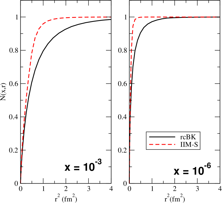
Figure 2: Pair separation dependence of the rcBK (solid line) and IIM (dashed line) scattering amplitudes at different values of $x$: (a) $x=10^{-3}$ and (b) $x=10^{-6}$.

The forward scattering amplitude ${\cal{N}}(x,\mbox{\boldmath$r$})$ is a solution of the Balitsky-Kovchegov (BK) equation, which is given in leading order by

$$\frac{\partial{{N}}(r,Y)}{\partial Y}=\int{\rm d}\bm{r_{1}}\,K^{\rm{LO}}(\bm{r,r_{1},r_{2}})[{{N}}(r_{1},Y)+{{N}}(r_{2},Y)-{{N}}(r,Y)-{{N}}(r_{1},Y){{N}}(r_{2},Y)],$$ (12)

where $Y\equiv\ln(x_{0}/x)$ ($x_{0}$ is the value of $x$ where the evolution starts), and $\bm{r_{2}=r-r_{1}}$. $K^{\rm{LO}}$ is the evolution kernel, given by

$$K^{\rm{LO}}(\bm{r,r_{1},r_{2}})=\frac{N_{c}\alpha_{s}}{2\pi^{2}}\frac{r^{2}}{r_{1}^{2}r_{2}^{2}},$$ (13)

where $\alpha_{s}$ is the strong coupling constant. This equation is a generalization of the linear BFKL equation (which corresponds of the first three terms), with the inclusion of the (non-linear) quadratic term, which damps the indefinite growth of the amplitude with energy predicted by BFKL evolution. The leading order BK equation presents some difficulties when applied to study DIS small-$x$ data. In particular, some studies concerning this equation IANCUGEO ; MT02 ; AB01 ; BRAUN03 ; AAMS05 have shown that the resulting saturation scale grows much faster with increasing energy ($\lambda\simeq 0.5$ ) than that extracted from phenomenology ($\lambda\simeq 0.2-0.3$). The calculation of the running coupling corrections to the BK evolution kernel was explicitly performed in kovwei1 ; balnlo , where the authors included $\alpha_{s}N_{f}$ corrections to the kernel to all orders. In bkrunning the improved BK equation was numerically solved replacing the leading order kernel in Eq. (12) by the modified kernel which includes the running coupling corrections and is given by balnlo

$$K^{\rm{Bal}}(\bm{r,r_{1},r_{2}})=\frac{N_{c}\alpha_{s}(r^{2})}{2\pi^{2}}\left[\frac{r^{2}}{r_{1}^{2}r_{2}^{2}}+\frac{1}{r_{1}^{2}}\left(\frac{\alpha_{s}(r_{1}^{2})}{\alpha_{s}(r_{2}^{2})}-1\right)+\frac{1}{r_{2}^{2}}\left(\frac{\alpha_{s}(r_{2}^{2})}{\alpha_{s}(r_{1}^{2})}-1\right)\right].$$ (14)

Numerical studies of the improved BK equation javier_kov have confirmed that the running coupling corrections lead to a considerable slow-down of the evolution speed, which implies, for example, a slower growth of the saturation scale with energy, in contrast with the faster growth predicted by the LO BK equation. Since the improved BK equation has been shown to be quite successful when applied to the description of the $ep$ HERA data for the proton structure function, we feel confident to use it in other physical situations such as $\gamma\gamma$ colisions. In what follows we make use of the public-use code available in code .

The running coupling Balitsky - Kovchegov (rcBK) predictions will be compared with those from the parametrization proposed in Ref. iim and updated in soyez , which was constructed so as to reproduce two limits of the LO BK equation analytically under control: the solution of the BFKL equation for small dipole sizes, $r\ll 1/Q_{s}(x)$, and the Levin-Tuchin law for larger ones, $r\gg 1/Q_{s}(x)$. In the updated version of this parametrization soyez , the free parameters were obtained by fitting more recent H1 and ZEUS data. In this parametrization the dipole forward scattering amplitude is given by

$${{N}}(x,\mbox{\boldmath$r$})=\left\{\begin{array}[]{ll}{\mathcal{N}}_{0}\,\left(\frac{r\,Q_{s}}{2}\right)^{2\left(\gamma_{s}+\frac{\ln(2/rQ_{s})}{\kappa\,\lambda\,Y}\right)}\,,&\mbox{for $rQ_{s}(x)\leq 2$}\,,\\ 1-\exp^{-a\,\ln^{2}\,(b\,r\,Q_{s})}\,,&\mbox{for $rQ_{s}(x)>2$}\,,\end{array}\right.$$ (17)

where $a$ and $b$ are determined by continuity conditions at $\mbox{\boldmath$r$}Q_{s}(x)=2$, $\gamma_{s}=0.6194$, $\kappa=9.9$, $\lambda=0.2545$, $Q_{0}^{2}=1.0$ GeV², $x_{0}=0.2131$ and ${\mathcal{N}}_{0}=0.7$. Hereafter, we shall call the model above IIM-S. The first line from Eq. (17) describes the linear regime whereas the second one describes saturation effects.

In Fig. 2 we compare the pair separation dependence of the rcBK and IIM-S forward dipole scattering amplitudes at distinct values of $x$. The main difference between these models is the rapid onset of saturation predicted by the IIM-S model. In comparison, the rcBK solution predicts a smooth growth, with a delayed saturation of the forward dipole scattering amplitude. Basically, the asymptotic saturation regime is only observed for very small values of $x$, beyond the kinematical range of HERA.

IV Results and discussion

Model	$N(\mbox{\boldmath$r$},Y)$	$m\,(\mbox{MeV})$	$\Lambda\,(\mbox{MeV})$
Model 1	rcBK	198	—
	IIM-S	205	—
Model 2	rcBK	—	210
	IIM-S	—	230

Table 1: Parameters used in the calculations.

Before presenting our results let us discuss the free parameters in our calculations. In the phenomenological model proposed in Kwien_Motyka , denoted in what follows Model 1, the parameter which is adjusted in order to describe the experimental data of the total $\gamma\gamma$ cross section is the mass of the light quarks. In order to describe the normalization of the data the authors are obliged to assume values which are larger than those obtained in the fit of the $F_{2}$ HERA data using the same phenomenological saturation model. Here we follow the same procedure and adjust the light quark mass in the wavefunctions in order to fit the real total cross section when using the rcBK and IIM-S models for the dipole scattering amplitude. On the other hand, when using the dipole scattering amplitude from Eq. (8), denoted Model 2 hereafter, we constrain the light quark mass to the values obtained in the original fits of the $F_{2}$ HERA data bkrunning ; soyez . However, in Model 2, due to the quadratic dependence on the size of the larger dipole [See Eq. (7)], the contribution of large values of $r_{1}$ and $r_{2}$ is quite significant in the total cross section. In order to keep our calculations in the perturbative regime we cut the integration on the pair separation at a maximum value of the order of the inverse perturbative QCD energy scale. In other words, we stop the $r_{1}$ and $r_{2}$ integrations at a maximum dipole size, which is chosen to be $r_{max}=\frac{1}{\Lambda}$, with $\Lambda$ a free parameter in the model which is expected to be $\approx\Lambda_{QCD}$. This parameter will be fitted in order to describe the total $\gamma\gamma$ cross section data at high energies. In principle we could keep $\Lambda=\Lambda_{QCD}$ fixed, understanding it as a clean-cut frontier between perturbative and non-perturbative physics. We could then compute the photon-photon cross sections, compare them with data and observe how well perturbative QCD works in this domain. Discrepancies between theory and data would be attributed to non-perturbative contributions. We expect these contributions to be larger in the case of real photons, which have a larger average transverse radius. However the uncertainties in the value of $\Lambda_{QCD}$ would make this separation between the perturbative and non-perturbative regimes less precise. In the present work we adjust the value of $\Lambda$. If the value required to fit the data would be much different (e.g. much smaller) from $\Lambda_{QCD}$ this would be an indication that it is not possible to describe the bulk of data only with perturbative QCD. Surprisingly the obtained values of $\Lambda$, shown in Table I, are close to the most accepted values of $\Lambda_{QCD}$, suggesting that the physics of high energy photon-photon scattering is to a large extent perturbative.

In Fig. 3 we present a comparison between the predictions obtained using the two models for $\sigma^{dd}$ and $N(r,Y)$ and the current experimental data for the total $\gamma\gamma$ cross section at high energies, where for instance rcBK(1) indicates that we are using the rcBK solution for the scattering and the Model 1 for the dipole-dipole cross section and so on. It is important to emphasize that differently from Kwien_Motyka , the Reggeon contributions are not included in our calculations, since our focus is in the energy range $W\geq 50$ GeV, where these contributions are very small. The parameters used in our calculations are presented in Table 1. As in Kwien_Motyka , the description of the experimental data l3_real using the Model 1 is only possible if we assume larger values of the light quark mass in comparison to those used in the description of the $F_{2}$ data, where $m_{u,d,s}=140$ MeV. On the other hand, the value of $\Lambda$ necessary to describe the experimental data is almost equal to $\Lambda_{QCD}$, in agreement with our expectations. This result can be interpreted as an indication that Model 2 for the dipole - dipole cross section captures the main features of the interaction. Finally, the predictions of the two models for $\sigma^{dd}$ are very similar in the kinematical range of the experimental data, independently of the $N(r,Y)$ considered. However, at $W>110$ GeV, the predictions are very distinct. In particular, at $W=1000$ GeV they differ by $\gtrsim 25$ %, with Model 2 predicting smaller values for the total $\gamma\gamma$ cross section.

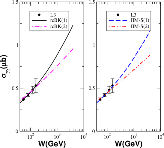
Figure 3: The total $\gamma\gamma$ cross section as a function of the energy $W$ for different models of dipole-dipole cross section and dipole scattering amplitude.

We can also compute the two-photon cross section for the case $Q_{1}^{2}\sim Q_{2}^{2}$ (with large $Q_{1,2}^{2}$) corresponding to the interaction of two (highly) virtual photons and also for the case $Q_{1}^{2}\gg Q_{2}^{2}$ corresponding to probing the structure of virtual ($Q_{2}^{2}>0$) or real ($Q_{2}^{2}=0$) photon at small values of the Bjorken parameter $x=Q_{1}^{2}/(2q_{1}q_{2})$ ($Q_{i}^{2}\equiv-q_{i}^{2}$). For instance, the structure function $F_{2}^{\gamma}(x,Q^{2})$ of the real photon ($Q_{2}^{2}=0,Q_{1}^{2}=Q^{2}$) is related in the following way to the $\gamma^{*}\gamma$ total cross-sections:

$$F_{2}^{\gamma}(x,Q^{2})\;=\;{Q^{2}\over 4\pi^{2}\alpha_{em}}[\sigma_{T,T}(W^{2},Q^{2},Q_{2}^{2}=0)+\sigma_{L,T}(W^{2},Q^{2},Q_{2}^{2}=0)].$$ (18)

In Fig. 4 we present our predictions for the total $\gamma^{*}\gamma^{*}$ cross section for different photon virtualities. We assume that $Q_{1}^{2}=Q_{2}^{2}=Q^{2}$ and analyse the dependence of the cross section on the variable $Y\equiv\ln(W^{2}/Q_{1}Q_{2})$. We can see that the cross sections increase with $Y$ and decrease with $Q^{2}$. Moreover, similarly to the real case, the main difference between the predictions is associated to the choice of $\sigma^{dd}$, with Model 1 predicting larger values for the cross section and a steeper growth in rapidity. This difference increases at larger values of the photon virtuality, being a factor $\approx 8$ for $Y=10$ and $Q^{2}=20$ GeV². The experimental point in the right panel is from the L3 Collaboration l3_virtual .

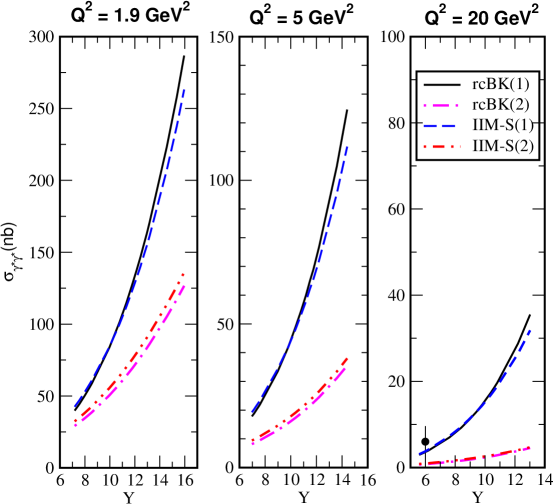
Figure 4: The total $\gamma^{*}\gamma^{*}$ cross sections as a function of the variable $Y\equiv\ln(W^{2}/Q_{1}Q_{2})$ for different values of $Q^{2}$ ($Q^{2}=Q_{1}^{2}=Q_{2}^{2}$).

Finally, in Fig. 5 we present our predictions for the $x$ dependence of the photon structure function $F_{2}^{\gamma}(x,Q^{2})$ for different values of the photon virtualities. The basic idea is that the quasi-real photon structure may be probed by other photon with a large momentum transfer. We present in the lower right panel our predictions for the virtual photon structure function. Although there exist only very few data on this observable, its experimental study is feasible in future linear colliders. Our results predict that $F_{2}^{\gamma}(x,Q^{2})$ increases at small-$x$, similarly to predictions for the proton structure function. The current experimental data f2_gama are described quite well. As it was seen previously in the case of $\sigma_{\gamma\gamma}$ and $\sigma_{\gamma^{*}\gamma^{*}}$, Model 1 predicts a steeper growth with the energy and, consequently, at smaller values of $x$, with the difference between the models increasing at larger values of $Q^{2}$. An important aspect is that the predictions obtained using Model 1 are almost independent of the scattering amplitude used in the calculations. On the other hand, in Model 2, the predictions depend more strongly on $N(\mbox{\boldmath$r$},Y)$. This makes the study of $F_{2}^{\gamma}(x,Q^{2})$ an important source of information about the QCD dynamics at high energies.

V summary

In this paper we have estimated the main observables to be studied in $\gamma\gamma$ collisions in the future linear colliders using the color dipole picture. In this approach the main input is the dipole - dipole cross section, which is determined by the QCD dynamics. We have discussed this quantity in detail and have introduced a new relation with the dipole scattering amplitude. In our calculations we use the state-of-the-art of the non-linear QCD dynamics, with the dipole scattering amplitude given by the solution of the running coupling Balitsky-Kovchegov equation which are compared with the predictions of the phenomenological saturation model proposed in iim and updated in soyez . Moreover, we compare our predictions with those obtained using the phenomenological model for the dipole - dipole cross section proposed in Kwien_Motyka . We demonstrate that these models are able to describe the scarce experimental data at currently available energies. However, they differ largely at higher energies, which implies that future experimental data could be used to constrain the QCD dynamics.

Figure 5: The photon structure function $F_{2}^{\gamma}(x,Q^{2})$ as a function of $x$ for different choices of the virtualities $Q_{1}^{2}$ and $Q_{1}^{2}$.

- (1) A. H. Mueller, Nucl. Phys. B415, 373 (1994); A. H. Mueller and B. Patel, Nucl. Phys. B425, 471 (1994); N. N. Nikolaev and B. G. Zakharov, Z. Phys. C49, 607 (1991); Z. Phys. C53, 331 (1992) .
- (2) L. N. Lipatov, Sov. J. Nucl. Phys. 23, 338 (1976); E. A. Kuraev, L. N. Lipatov, V. S. Fadin, JETP 45, 1999 (1977); I. I. Balitskii, L. N. Lipatov, Sov. J. Nucl. Phys. 28, 822 (1978).
- (3) F. Gelis, E. Iancu, J. Jalilian-Marian and R. Venugopalan, arXiv:1002.0333 [hep-ph];E. Iancu and R. Venugopalan, arXiv:hep-ph/0303204; A. M. Stasto, Acta Phys. Polon. B 35, 3069 (2004); H. Weigert, Prog. Part. Nucl. Phys. 55, 461 (2005); J. Jalilian-Marian and Y. V. Kovchegov, Prog. Part. Nucl. Phys. 56, 104 (2006).
- (4) Y. V. Kovchegov and H. Weigert, Nucl. Phys. A 784, 188 (2007); Nucl. Phys. A 789, 260 (2007); Y. V. Kovchegov, J. Kuokkanen, K. Rummukainen and H. Weigert, Nucl. Phys. A 823, 47 (2009).
- (5) J. L. Albacete and Y. V. Kovchegov, Phys. Rev. D 75, 125021 (2007).
- (6) I. Balitsky, Phys. Rev. D 75, 014001 (2007); I. Balitsky and G. A. Chirilli, Phys. Rev. D 77, 014019 (2008).
- (7) J. L. Albacete, N. Armesto, J. G. Milhano and C. A. Salgado, Phys. Rev. D80, 034031 (2009).
- (8) H. Weigert, J. Kuokkanen and K. Rummukainen, AIP Conf. Proc. 1105, 394 (2009).
- (9) M. A. Betemps, V. P. Goncalves and J. T. de Santana Amaral, Eur. Phys. J. C 66, 137 (2010).
- (10) V. P. Goncalves, M. V. T. Machado and A. R. Meneses, Eur. Phys. J. C 68, 133 (2010).
- (11) J. L. Albacete and C. Marquet, Phys. Lett. B 687, 174 (2010).
- (12) R. Nisius, Phys. Rept. 332, 165 (2000).
- (13) J. Bartels, A. De Roeck, H. Lotter, Phys. Lett. B 389, 742 (1996); J. Bartels, C. Ewerz, R. Staritzbichler, Phys. Lett. B 492, 56 (2000); A. Bialas, W. Czyz, W. Florkowski, Eur. Phys. J. C 2, 683 (1998); J. Kwiecinski, L. Motyka, Eur. Phys. J. C 18, 343 (2000); N. N. Nikolaev, B. G. Zakharov, V. R. Zoller, JETP 93, 957 (2001); S. J. Brodsky, F. Hautmann, D. E. Soper, Phys. Rev. D 56, 6957 (1997); Phys. Rev. Lett. 78, 803 (1997).
- (14) M. Boonekamp, A. De Roeck, C. Royon, S. Wallon, Nuc. Phys. B 555, 540 (1999).
- (15) S.J. Brodsky, V.S. Fadin, V.T. Kim, L.N. Lipatov, G.B. Pivovarov, Pis’ma ZHETF 76, 306 (2002) [JETP Letters 76, 249 (2002)].
- (16) V. P. Goncalves, M. V. T. Machado and W. K. Sauter, J. Phys. G 34, 1673 (2007)
- (17) F. Caporale, D. Y. Ivanov and A. Papa, Eur. Phys. J. C 58, 1 (2008)
- (18) K. Golec-Biernat and M. Wüsthoff, Phys. Rev. D 60, 114023 (1999); Phys. Rev. D 59, 014017 (1998).
- (19) J. Bartels, K. Golec-Biernat and H. Kowalski, Phys. Rev D66, 014001 (2002) .
- (20) H. Kowalski and D. Teaney, Phys. Rev. D 68, 114005 (2003).
- (21) H. Kowalski, L. Motyka and G. Watt, Phys. Rev. D 74, 074016 (2006).
- (22) J. R. Forshaw, R. Sandapen and G. Shaw, Phys. Lett. B 594, 283 (2004).
- (23) J. R. Forshaw, R. Sandapen and G. Shaw, JHEP 0611, 025 (2006).
- (24) D. Kharzeev, Y.V. Kovchegov and K. Tuchin, Phys. Lett. B599, 23 (2004).
- (25) E. Iancu, K. Itakura, S. Munier, Phys. Lett. B 590, 199 (2004).
- (26) A. Dumitru, A. Hayashigaki and J. Jalilian-Marian, Nucl. Phys. A765, 464 (2006); Nucl.Phys. A770, 57 (2006).
- (27) V. P. Goncalves, M. S. Kugeratski, M. V. T. Machado and F. S. Navarra, Phys. Lett. B 643, 273 (2006).
- (28) C. Marquet, R. B. Peschanski and G. Soyez, Phys. Rev. D 76, 034011 (2007).
- (29) C. Marquet, Phys. Rev. D 76, 094017 (2007) .
- (30) D. Boer, A. Utermann and E. Wessels, Phys. Rev. D 77, 054014 (2008).
- (31) G. Soyez, Phys. Lett. B 655, 32 (2007).
- (32) G. Watt and H. Kowalski, Phys. Rev. D 78, 014016 (2008).
- (33) N. Timneanu, J. Kwiecinski, L. Motyka, Eur. Phys. J. C 23, 513 (2002).
- (34) N. N. Nikolaev, J. Speth and V. R. Zoller, Eur. Phys. J. C 22, 637 (2002); J. Exp. Theor. Phys. 93, 957 (2001) [Zh. Eksp. Teor. Fiz. 93, 1104 (2001)].
- (35) A. Donnachie, H. G. Dosch and M. Rueter, Phys. Rev. D 59, 074011 (1999).
- (36) J. L. Albacete, N. Armesto, J. G. Milhano, P. Q. Arias and C. A. Salgado, arXiv:1012.4408 [hep-ph].
- (37) A.H. Mueller and A.I. Shoshi, Nucl. Phys. B 692, 175 (2004); E. Iancu, A.H. Mueller and S. Munier, Phys. Lett. B 606, 342 (2005); E. Iancu and D.N. Triantafyllopoulos, Nucl. Phys. A 756, 419 (2005); A.H. Mueller, A.I. Shoshi and S.M.H.Wong, Nucl. Phys. B 715, 440 (2005); E. Iancu and D.N. Triantafyllopoulos, Phys. Lett. B 610, 253 (2005); E. Levin and M. Lublinsky, Nucl. Phys. A 763, 172 (2005); A. Kovner and M. Lublinsky, Phys. Rev. D 71, 085004 (2005); A. Kovner and M. Lublinsky, Phys. Rev. Lett. 94, 181603 (2005); E. Iancu, Y. Hatta, C. Marquet, G. Soyez and D.N. Triantafyllopoulos, Nucl. Phys. A 773, 95 (2006).
- (38) A. Dumitru, E. Iancu, L. Portugal, G. Soyez and D. N. Triantafyllopoulos, JHEP 0708, 062 (2007)
- (39) H. Navelet and S. Wallon, Nucl. Phys. B 522, 237 (1998)
- (40) A. H. Mueller and G. P. Salam, Nucl. Phys. B 475, 293 (1996)
- (41) E. Iancu and A. H. Mueller, Nucl. Phys. A 730, 460 (2004); G. P. Salam, Nucl. Phys. B 461, 512 (1996)
- (42) E. Iancu, M. S. Kugeratski and D. N. Triantafyllopoulos, Nucl. Phys. A 808, 95 (2008).
- (43) E. Iancu, K. Itakura and L. McLerran, Nucl. Phys A708, 327 (2002).
- (44) A. H. Mueller and D. N. Triantafyllopoulos, Nucl. Phys. B640, 331 (2002).
- (45) N. Armesto and M. A. Braun, Eur. Phys. J. C20, 517 (2001).
- (46) M. A. Braun, Phys. Lett. B 576, 115 (2003).
- (47) J. L. Albacete, N. Armesto, J. G. Milhano, C. A. Salgado, and U. A. Wiedemann, Phys. Rev. D 71, 014003 (2005).
- (48) http://www-fp.usc.es/phenom/rcbk
- (49) M. Acciarri et al. [L3 Collaboration], Phys. Lett. B 519, 33 (2001)
- (50) M. Acciarri et al. [L3 Collaboration], Phys. Lett. B 453, 333 (1999).
- (51) M. Acciarri et al. [L3 Collaboration], Phys. Lett. B 447, 147 (1999) ; G. Abbiendi et al. [OPAL Collaboration], Eur. Phys. J. C 18, 15 (2000) .