Simultaneous time-optimal control of the inversion of two spin 1/2 particles

Abstract

We analyze the simultaneous time-optimal control of two-spin systems. The two non coupled spins which differ in the value of their chemical offsets are controlled by the same magnetic fields. Using an appropriate rotating frame, we restrict the study to the case of opposite shifts. We then show that the optimal solution of the inversion problem in a rotating frame is composed of a pulse sequence of maximum intensity and is similar to the optimal solution for inverting only one spin by using a non-resonant control field in the laboratory frame. An example is implemented experimentally using techniques of Nuclear Magnetic Resonance.

1 Introduction

Since its discovery in 1945 by Purcell, Torrey and Pound, Nuclear Magnetic Resonance (NMR) has become a powerful physical tool to study molecules and matter in a variety of domains extending from biology and chemistry to solid physics and quantum mechanics [1]. NMR involves the manipulation of nuclear spins via its interaction with a magnetic field, and is therefore a domain where techniques of quantum control can be applied (see [2] and references therein). Such an approach has many potential applications ranging from the improvement of the resolution and sensitivity of NMR spectroscopy experiments [3] to quantum computing [4]. The control technology developed over the past fifty years allows the use of sophisticated control fields for spectroscopy and also permits the implementation of complex quantum algorithms [5].

In this context, some challenging control problems are raised by the experimental constraints of NMR experiments. Roughly speaking, the measured signal is the magnetization of a sample which is produced by a large number of spin systems. One usually assumes in simple models that the static magnetic field is the same across the sample, i.e. the field is perfectly homogeneous with respect to the different spins. This is not always true in practice since for technical reasons it is difficult to generate homogeneous fields. Even in the situation where the magnetic field is uniform on a macroscopic scale, the interaction between the different atoms (or between a spin and its environment) induces a chemical shift on the frequency transition of a given spin. This leads classically to an unwanted rotation of each individual spin around a fixed axis which is not taken into account in the simplest model of spin 1/2 particles. The shift being different for each spin, the rotation is different for each spin. Note that this effect is useful in NMR spectroscopy since it encodes in a sense some informations about the structure of the molecules. The consequences are negative from a control point of view since this phenomenon decreases the efficiency of the control field. The objective is therefore to find controls able to bring the system towards a given target state in a sufficiently robust way with respect to inhomogeneities of the transition frequency. This problem has been solved numerically in different works [15] leading to very efficient but complicated solutions. In particular, no insight into the control mechanism is gained from this approach and no optimality result has been proven. Note that some related works have been done in the control of molecular dynamics by laser fields [16] by using monotonically convergent algorithms [17].

In this paper, we propose to revisit this problem by using techniques of geometric optimal control theory [6, 7]. Geometric optimal control is a vast domain based on the application of the Pontryagin Maximum Principle (PMP) where the idea is to use the methods of differential geometry and Hamiltonian dynamics to solve the optimal control problems [6, 7]. This geometric framework leads to a global analysis of the control problem which completes and guides the numerical computations. Some geometric results on the optimal control of spin systems have been first obtained by N. Khaneja and his co-workers [12]. Recently, the time-optimal control of dissipative spin 1/2 particles has been solved theoretically [14] and implemented experimentally [13]. In this work we study the simultaneous control of two non-interacting spins with different resonance frequencies. More precisely, we consider as an example the problem to simultaneously invert the magnetization vectors initially aligned along the $z$- axis defined by the direction of the static magnetic field.

Using an appropriate rotating frame, we show that we can always consider the symmetric case where the two transition frequencies are opposed. In this situation, the time-optimal solution for inverting the two spins by the same transverse radiofrequency (rf) control fields is a bang-bang pulse sequence in a frame rotating at the rf frequency. The remarkable point is that the co-rotating component of the applied rf field is the same as the one used to invert only one spin with one non-resonant control field in the laboratory frame [9]. We finally implement experimentally the optimal solution by using techniques of NMR.

The paper is organized as follows. In Sec. 2, we recall the tools to control one spin in minimum time with a transverse magnetic field which is not in resonance with the frequency of the spin. In Sec. 3, we establish that this control field is also the optimal solution to simultaneously invert two spins. An experimental illustration is given in Sec. 4. A summary of the different results obtained is presented in Sec. 5.

2 Time-optimal control of a spin 1/2 particle

We consider the control of a spin 1/2 particle whose dynamics is governed by the Bloch equation:

$$\left(\begin{array}[]{c}\dot{M}_{x}\\ \dot{M}_{y}\\ \dot{M}_{z}\end{array}\right)=\left(\begin{array}[]{c}-\omega M_{y}\\ \omega M_{x}\\ 0\end{array}\right)+\left(\begin{array}[]{c}0\\ -\omega_{x}M_{z}\\ \omega_{x}M_{y}\end{array}\right)$$ (1)

where $\vec{M}$ is the magnetization vector and $\omega$ the chemical shift offset. The dynamics is controlled through only one magnetic field along the $x$- axis which satisfies the constraint $\omega_{x}\leq\omega_{max}$. We introduce normalized coordinates $\vec{x}=(x,y,z)=\vec{M}/M_{0}$ where $\vec{M}_{0}=M_{0}\vec{e}_{z}$ is the thermal equilibrium point, a normalized control field $u_{x}=2\pi\omega_{x}/\omega_{max}$ which satisfies the constraint $u_{x}\leq 2\pi$ and a normalized time $\tau=\omega_{max}t/(2\pi)$. Dividing the previous system by $\omega_{max}M_{0}/(2\pi)$, we get that the evolution of the normalized coordinates is given by the following equations:

$$\left(\begin{array}[]{c}\dot{x}\\ \dot{y}\\ \dot{z}\end{array}\right)=\left(\begin{array}[]{c}-\Delta y\\ \Delta x\\ 0\end{array}\right)+\left(\begin{array}[]{c}0\\ -u_{x}z\\ u_{x}y\end{array}\right)$$ (2)

where $\Delta$ is the normalized offset given by $\Delta=2\pi\omega/\omega_{max}$.

The complete description of the time-optimal control problem of a spin 1/2 particle by a non-resonant magnetic field is done in Ref. [9]. In this section, we give only a brief summary of the results of this paper which will be used in our study. The reader is referred to [9] for the different proofs of these results. Note that when the spin is controlled by two magnetic fields, respectively along the $x$ and $y$ directions, then the system is equivalent to a two-level quantum system in the rotating wave approximation [8]. This means that a unitary transformation can be used to remove the drift term depending on $\Delta$. In this case, the optimal control field is a $\pi$-pulse.

The problem we consider belongs to a general class of optimal control problems for which powerful mathematical tools have been developed [10]. They correspond to systems on a two-dimensional manifold (here the Bloch sphere) controlled by a single field. The evolution of the system is ruled by the following set of differential equations:

$$\dot{\vec{x}}=F(\vec{x})+uG(\vec{x})$$ (3)

where $\vec{x}$ is the two-dimensional state vector and $u$ the control field which satisfies the constraint $u\leq u_{0}$ with, here, $u_{0}=2\pi$. The time-optimal control problem is solved by the application of the Pontryagin Maximum Principle (PMP) which is formulated using the pseudo-Hamiltonian

$$H=\vec{p}\cdot(F+uG)+p_{0},$$

where $\vec{p}$ is the adjoint state and $p_{0}$ a negative constant such that $\vec{p}$ and $p_{0}$ are not simultaneously equal to 0. The Pontryagin maximum principle states that the optimal trajectories are solutions of the equations

$$\begin{array}[]{lll}\dot{\vec{x}}=\frac{\partial H}{\partial\vec{p}}(\vec{x},\vec{p},v),\ \dot{\vec{p}}=-\frac{\partial H}{\partial\vec{x}}(\vec{x},\vec{p},v)\\ H(\vec{x},\vec{p},v)=\max_{|u|\leq u_{0}}H(\vec{x},\vec{p},u)\\ H(\vec{x},\vec{p},v)=0.\end{array}$$ (7)

Introducing the switching function $\Phi$ given by

$$\Phi(t)=\vec{p}\cdot G,$$

one deduces using the second equation of (7) that the optimal synthesis is composed of concatenation of arcs $\gamma_{+}$, $\gamma_{-}$ and $\gamma_{S}$. $\gamma_{+}$ and $\gamma_{-}$ are regular arcs corresponding respectively to $\textrm{sign}[\Phi(t)]=\pm 1$ or to the control fields $u=\pm u_{0}$. A switching from $u_{0}$ to $-u_{0}$ or from $-u_{0}$ to $u_{0}$ occurs at $t=t_{0}$ when the function $\Phi$ takes the value zero and when this zero is isolated. Singular arcs $\gamma_{s}$ are characterized by the fact that $\Phi$ vanishes on an interval $[t_{0},t_{1}]$. In this case, differentiating two times $\Phi$ with respect to time and imposing that the derivatives are zero, one obtains that the singular arcs are located in the set

$$S=\{\vec{x};\ \Delta_{S}(x)=\det(G,[G,F])(\vec{x})=0\}.$$

We recall that the commutator $[F,G]$ of two vector fields $F$ and $G$ is defined by:

$$[F,G]=\nabla F\cdot G-F\cdot\nabla G$$

where $\nabla$ is the gradient of a function. The singular control field $u_{s}$ can be calculated as a feedback control, i.e. as a function of the coordinates by imposing that the second derivative of $\Phi$ with respect to time is equal to 0:

$$[G,[G,F]]+u_{s}[F,[G,F]]=0.$$

The optimal solution can follow the singular lines if the control field is admissible, i.e. if $|u_{s}(\vec{x})|\leq u_{0}$.

Since the two-dimensional manifold of our control problem is the Bloch sphere, the adapted coordinates are the spherical ones:

$$\left\{\begin{array}[]{rcl}x&=&r\,\sin\theta\,\cos\phi\\ y&=&r\,\sin\theta\,\sin\phi\\ z&=&r\,\cos\theta\end{array}\right.,$$ (8)

which leads to the following system:

$$\left(\begin{array}[]{c}\dot{r}\\ \dot{\theta}\\ \dot{\phi}\end{array}\right)=\left(\begin{array}[]{c}0\\ 0\\ \Delta\end{array}\right)+u\left(\begin{array}[]{c}0\\ -\sin\,\phi\\ -\cos\,\phi\,\cot\,\theta.\end{array}\right)$$ (9)

The pseudo-Hamiltonian $H$ has the form:

$$H=\Delta\,p_{\phi}-u(\sin\,\phi\,p_{\theta}+\cos\,\phi\,\cot\,\theta\,p_{\phi}).$$ (10)

and the switching function is given by $\Phi=\sin\phi p_{\theta}+\cos\,\phi\,\cot\,\theta\,p_{\phi}$. Since

$$[G,F]=\left(\begin{array}[]{c}0\\ -\Delta\,\cos\,\phi\\ \Delta\,\sin\,\phi\,\cot\,\theta\end{array}\right)$$

one deduces that $S$ is the set

$$S=\left\{\vec{x}|\sin^{2}\phi\cot\theta=-\cos^{2}\phi\cot\theta\right\}=\left\{\vec{x}|\theta=\pi/2\right\},$$

i.e. the singular locus is the equator of the Bloch sphere. The time-optimal control problem is solved in [9]. It has been shown that the optimal solution reaching the south pole from the north pole is the succession of different bang pulses, i.e. of pulses of maximum intensity $2\pi$. The number of bangs is at most equal to 2 if $\Delta<2\pi$ and can be larger if $\Delta>2\pi$. The singular extremals play no role for this spin inversion. An example of an optimal pulse sequence and the corresponding trajectory is displayed in Figs. 1 and 2. The optimal trajectory is not smooth at switching points where the value of the control field changes. The switching times can analytically be determined using the material of Ref. [9]. In the case of Fig. 1, the optimal solution is a type-2-trajectory described by Proposition 5 of [9]. These times can also be computed numerically by solving a shooting equation. More precisely, this means that one has to determine the initial adjoint state $\vec{p}(0)=(p_{\theta}(0),p_{\phi}(0))$ such that the corresponding Hamiltonian trajectory $(\vec{x},\vec{p})$ with initial conditions $(\vec{x}(0),\vec{p}(0))$ goes to the target $\vec{x}_{f}$ at time $t_{f}$. This condition can be expressed as the determination of the roots of the equation $\vec{x}(t_{f})[\vec{p}(0)]-\vec{x}_{f}$ which can be solved if one has a sufficiently good approximation of $\vec{p}(0)$ by a standard Newton-type algorithm. Note that the control field is determined along the trajectory by computing the switching function $\Phi$.

At this point, we can extend the previous discussion as a first step towards the simultaneous inversion of two spins. We analyze the dynamics in a rotating frame by using the rotating wave approximation (RWA) where the offsets of the two spins are symmetric and given by $\pm\Delta$. The rf field is assumed to be at the rotating frame frequency. As a consequence of the symmetries of the problem, one sees that if $u(t)$, the co-rotating component of the applied rf field, steers the spin with offset $\Delta$ from the north pole to the south pole then the same field will also invert the other spin. The trajectories of the two spins in the $y$- and $z$- directions will be the same, while it will be opposite along the $x$- axis. Note that this solution is not the unique solution and a family of solutions satisfying the same requirement can be determined. Consider the set of control fields defined by

$$\left\{\begin{array}[]{rcl}u_{x}=u(t)\cos\alpha\\ u_{y}=u(t)\sin\alpha\\ \end{array}\right.$$ (11)

where $\alpha\in[0,2\pi]$. If we consider the following rotation $R(\alpha)$ of angle $\alpha$ along the $z$- axis:

$$\left(\begin{array}[]{c}X\\ Y\\ Z\\ \end{array}\right)=\left(\begin{array}[]{ccc}\cos\alpha&\sin\alpha&0\\ -\sin\alpha&\cos\alpha&0\\ 0&0&1\\ \end{array}\right)\left(\begin{array}[]{c}x\\ y\\ z\\ \end{array}\right)$$ (12)

then the new system in the coordinates $(X,Y,Z)$ is controlled by a single field $u(t)$ along the $X$- direction. It is also straightforward to see that this solution is the optimal one for the inversion control of two symmetric spins by one control field.

The question that we ask now is whether this simple solution is the optimal solution of the simultaneous inversion of two spins when two control fields are considered.

3 Simultaneous control of the inversion of two spin 1/2 particles

3.1 The model system

We consider two different spin 1/2 particles with the offsets $\omega_{a}$ and $\omega_{b}$. Using the same normalization as in Sec. 2 and the RWA, one arrives to the following equations:

$$\left(\begin{array}[]{c}\dot{x}_{a}\\ \dot{y}_{a}\\ \dot{z}_{a}\\ \dot{x}_{b}\\ \dot{y}_{b}\\ \dot{z}_{b}\end{array}\right)=\left(\begin{array}[]{c}-\Delta_{a}y_{a}\\ \Delta_{a}x_{a}\\ 0\\ -\Delta_{b}y_{b}\\ \Delta_{b}x_{b}\\ 0\end{array}\right)+u_{x}\left(\begin{array}[]{c}0\\ -z_{a}\\ y_{a}\\ 0\\ -z_{b}\\ y_{b}\end{array}\right)+u_{y}\left(\begin{array}[]{c}z_{a}\\ 0\\ -x_{a}\\ z_{b}\\ 0\\ -x_{b}\end{array}\right)$$ (13)

where the coordinates $(x_{a},y_{a},z_{a})$ and $(x_{b},y_{b},z_{b})$ are respectively associated to the first and second spins $a$ and $b$. The parameters $\Delta_{a}$ and $\Delta_{b}$ are the offsets of the spins $a$ and $b$ with respect to the frequency of the rotating frame. The rf field is here also at the rotating frame frequency. We assume that the two spins have the same equilibrium point $M_{0}$. As mentioned below, two magnetic fields along the $x$- and $y$- directions are taken into account in this problem. They satisfy the constraints $\sqrt{u_{x}^{2}+u_{y}^{2}}\leq 2\pi$. Using a rotating frame that rotates at frequency $(\Delta_{a}+\Delta_{b})/2$, it is straightforward to transform this system into a symmetric one where the frequencies of the two spins are opposite. This is the case analyzed below.

We introduce the spherical coordinates for the two spins and we get:

$$\left(\begin{array}[]{c}\dot{r_{a}}\\ \dot{\theta_{a}}\\ \dot{\phi_{a}}\\ \dot{r_{b}}\\ \dot{\theta_{b}}\\ \dot{\phi_{b}}\\ \end{array}\right)=\left(\begin{array}[]{c}0\\ 0\\ \Delta\\ 0\\ 0\\ -\Delta\end{array}\right)+u_{x}G_{x}+u_{y}G_{y}$$ (14)

where

$$G_{x}=\left(\begin{array}[]{c}0\\ -\sin\phi_{a}\\ -\cot\theta_{a}\,\cos\phi_{a}\\ 0\\ -\sin\phi_{b}\\ -\cot\theta_{b}\,\cos\phi_{b}\end{array}\right),~{}G_{y}=\left(\begin{array}[]{c}0\\ \cos\,\phi_{a}\\ -\cot\theta_{a}\,\sin\phi_{a}\\ 0\\ \cos\,\phi_{b}\\ -\cot\theta_{b}\,\sin\phi_{b}\end{array}\right).$$

Since the radial coordinates $(r_{a},r_{b},p_{r_{a}},p_{r_{b}})$ play a trivial role in this problem, we omit them in the following equations.

We apply the PMP to this system in the time-optimal case and we obtain the following pseudo-Hamiltonian

$$H=\Delta(p_{\phi_{a}}-p_{\phi_{b}})+\vec{p}\cdot(u_{x}G_{x}+u_{y}G_{y})$$ (15)

where $\vec{p}$ is the adjoint vector of coordinates $(p_{\theta_{a}},p_{\phi_{a}},p_{\theta_{b}},p_{\phi_{b}})$. In the normal case, the optimization condition leads to the following optimal controls:

$$u_{x}=\frac{\vec{p}\cdot G_{x}}{\sqrt{(\vec{p}\cdot G_{x})^{2}+(\vec{p}\cdot G_{y})^{2}}},~{}u_{y}=\frac{\vec{p}\cdot G_{y}}{\sqrt{(\vec{p}\cdot G_{x})^{2}+(\vec{p}\cdot G_{y})^{2}}},$$ (16)

where $\vec{p}\cdot G_{x}$ and $\vec{p}\cdot G_{y}$ are not simultaneously equal to 0. The singular case occurs when $\vec{p}\cdot G_{x}=\vec{p}\cdot G_{y}=0$, which defines the switching surface $\Sigma$. In the two-control problems, singular trajectories are the trajectories which lie on $\Sigma$. We assume in this paper that these controls do not play any role in our problem. This is expected since singular extremals are not generically optimal for a two-control problem [18].

We get the normal Hamiltonian $H_{n}$ by replacing the control fields by their expressions:

$$H_{n}=\Delta(p_{\phi_{a}}-p_{\phi_{b}})+\sqrt{(\vec{p}\cdot G_{x})^{2}+(\vec{p}\cdot G_{y})^{2}}.$$ (17)

The normal extremals will be given by the Hamiltonian trajectories of $H_{n}$. The next step of our study will consists in the analysis of this Hamiltonian flow.

For that purpose, we introduce the following canonical transformation on the $\phi$- coordinates:

$$\left\{\begin{array}[]{rcl}\phi_{+}&=&\phi_{a}+\phi_{b}\\ \phi_{-}&=&\phi_{a}-\phi_{b}\\ \end{array}\right.$$ (18)

which is defined through the generating function:

$$F_{2}=\frac{1}{2}p_{\phi_{a}}(\phi_{+}+\phi_{-})+\frac{1}{2}p_{\phi_{b}}(\phi_{+}-\phi_{-})$$

with the transformation:

$$p_{\phi_{+}}=\frac{\partial F_{2}}{\partial\phi_{+}};~{}p_{\phi_{-}}=\frac{\partial F_{2}}{\partial\phi_{-}};~{}\phi_{a}=\frac{\partial F_{2}}{\partial p_{\phi_{a}}};~{}\phi_{b}=\frac{\partial F_{2}}{\partial p_{\phi_{b}}}.$$

This leads to

$$\left\{\begin{array}[]{rcl}p_{\phi_{a}}&=&p_{\phi_{+}}+p_{\phi_{-}}\\ p_{\phi_{b}}&=&p_{\phi_{+}}-p_{\phi_{-}}\\ \end{array}\right..$$ (19)

The Hamiltonian $H_{n}$ expressed in the new set of coordinates does not depend of $\phi_{+}$, so $p_{\phi_{+}}$ is a constant of the motion. Since at the initial time in the north pole, $p_{\phi_{a}}(0)=p_{\phi_{b}}(0)=0$, one deduces that $p_{\phi_{+}}=0$. One finally arrives at

$$H_{n}=2\Delta p_{\phi_{-}}+[p_{\theta_{a}}^{2}+p_{\theta_{b}}^{2}+p_{\phi_{-}}^{2}(\cot^{2}\theta_{a}+\cot^{2}\theta_{b})$$

$$+2\cos\phi_{-}(p_{\theta_{a}}p_{\theta_{b}}-p_{\phi_{-}}^{2}\cot\theta_{a}\cot\theta_{b})$$

$$-2p_{\phi_{-}}\sin\phi_{-}(p_{\theta_{a}}\cot\theta_{b}-p_{\theta_{b}}\cot\theta_{a})]^{1/2}.$$

Care has to be taken with the use of these coordinates on the poles of the sphere. On a pole, we have $\cot\theta\to\pm\infty$ and $p_{\phi}=0$ but the product $p_{\phi}\cot\theta$ remains finite. In this paper, spherical coordinates are only used to describe the geometric properties of the extremals and to highlight their symmetries. All the numerical computations are done in cartesian coordinates.

Note also the symmetric role played by $\theta_{a}$ and $\theta_{b}$ in the Hamiltonian $H_{n}$. This symmetry will be used in the proof below.

3.2 The optimal control problem

We first analyze the characteristics of the extremal trajectories which are solutions of the control problem. In particular, if the inversion is realized by an extremal trajectory then the following relations are satisfied:

$$\forall t\in[0,t_{f}],p_{\theta_{a}}(t)=p_{\theta_{b}}(t)~{}\textrm{and}~{}\theta_{a}(t)=\theta_{b}(t),$$

where $t_{f}$ is the control duration.

To show this property, we assume that the south pole is reached by the extremal. In this case, the final point satisfies by definition:

$$\theta_{a}(t_{f})=\theta_{b}(t_{f}),~{}\dot{\theta}_{a}(t_{f})=\dot{\theta}_{b}(t_{f}),p_{\phi_{-}}=0.$$

Using the Hamiltonian $H_{n}$, we obtain:

$$\left\{\begin{array}[]{rcl}\dot{\theta_{a}}=\frac{\partial H_{n}}{\partial p_{\theta_{a}}}=(p_{\theta_{a}}+\cos\phi_{-}p_{\theta_{b}}-p_{\phi_{-}}\sin\phi_{-}\cot\theta_{b})/\sqrt{Q}\\ \dot{\theta_{b}}=\frac{\partial H_{n}}{\partial p_{\theta_{b}}}=(p_{\theta_{b}}+\cos\phi_{-}p_{\theta_{a}}-p_{\phi_{-}}\sin\phi_{-}\cot\theta_{a})/\sqrt{Q}\\ \end{array}\right.,$$ (20)

where

$$Q=p_{\theta_{a}}^{2}+p_{\theta_{b}}^{2}+p_{\phi_{-}}^{2}(\cot^{2}\theta_{a}+\cot^{2}\theta_{b})$$

$$+2\cos\phi_{-}(p_{\theta_{a}}p_{\theta_{b}}-p_{\phi_{-}}^{2}\cot\theta_{a}\cot\theta_{b})$$

$$-2p_{\phi_{-}}\sin\phi_{-}(p_{\theta_{a}}\cot\theta_{b}-p_{\theta_{b}}\cot\theta_{a}).$$

We consider that $Q(0)\neq 0$ which is always possible by a judicious choice of the initial adjoint vector $\vec{p}(0)$. This implies that $H_{n}>0$ since $p_{\phi_{-}}=0$ at a pole. Using the fact that $H_{n}$ is a constant of motion, one deduces at the final point that $Q(t_{f})\neq 0$. From Eqs. (20), one finally arrives at

$$(p_{\theta_{a}}(t_{f})-p_{\theta_{b}}(t_{f}))(1-\cos\phi_{-}(t_{f}))=0.$$

If $\cos\phi_{-}(t_{f})=1$ then $Q=0$, which is not possible from our hypothesis. We have therefore $p_{\theta_{a}}(t_{f})=p_{\theta_{b}}(t_{f})$ and using the Hamiltonian equations, we then obtain that $\theta_{a}(t)=\theta_{b}(t)$ and $p_{\theta_{a}}(t)=p_{\theta_{b}}(t)$ for any time $t$ since at time $t=t_{f}$ we have $\theta_{a}(t_{f})=\theta_{b}(t_{f})$ and $p_{\theta_{a}}(t_{f})=p_{\theta_{b}}(t_{f})$.

We also get that $\dot{\phi}_{+}=0$, i.e. $\phi_{+}=\phi_{+0}$. In the new coordinates $\vec{X}_{a}$ and $\vec{X}_{b}$ such that $\vec{X}_{a}=R(\phi_{+0}/2)\vec{x}_{a}$ and $\vec{X}_{b}=R(\phi_{+0}/2)\vec{x}_{b}$, the sum of the new azimuthal angles is zero and we obtain the following symmetry on the trajectory:

$$\left\{\begin{array}[]{rcl}X_{a}(t)&=&X_{b}(t)\\ Y_{a}(t)&=&-Y_{b}(t)\\ Z_{a}(t)&=&Z_{b}(t)\end{array}\right.$$ (21)

for any $t\in[0,t_{f}]$. In these coordinates, the two control fields are given by

$$\left\{\begin{array}[]{rcl}u_{X}(t)&=&u_{x}(t)\cos(\frac{\phi_{0}}{2})+u_{y}(t)\sin(\frac{\phi_{0}}{2})\\ u_{Y}(t)&=&-u_{x}(t)\sin(\frac{\phi_{0}}{2})+u_{y}(t)\cos(\frac{\phi_{0}}{2})\\ \end{array}\right.$$ (22)

From this symmetry, we have $u_{X}(t)=0$ and thus $u_{x}(t)\cos(\phi_{0+}/2)+u_{y}(t)\sin(\phi_{0+}/2)=0$. Since $u_{x}(t)^{2}+u_{y}(t)^{2}\leq 4\pi^{2}$, this leads to

$$\left\{\begin{array}[]{rcl}u_{x}(t)=u_{0}(t)\cos(\phi_{0+}/2)\\ u_{y}(t)=-u_{0}(t)\sin(\phi_{0+}/2)\end{array}\right.$$ (23)

where $u_{0}(t)$ is a bang-bang pulse of amplitude $2\pi$. We therefore recover the case of Sec. 2 of the optimal control of one spin system.

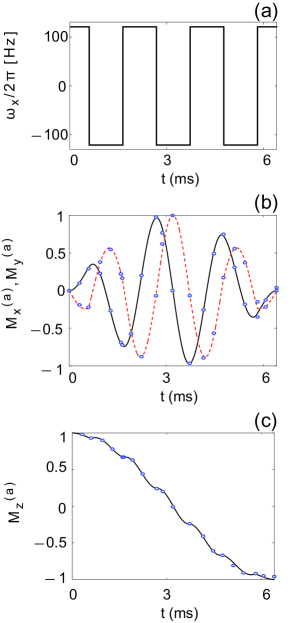
Figure 1: (Color Online) Panel (a): Plot of the optimal control field for the simultaneous inversion of two spins with offsets $\omega/2\pi=\pm 483$ Hz and $\omega_{max}/2\pi=120.75$ Hz. Panel (b): Plots of the corresponding optimal trajectories for $M_{x}^{a}(t)$ (solid black line) and $M_{y}^{a}(t)$ (red dashed line). The experimentally measured trajectories are presented by open circles. Panel (c): Plot of the optimal trajectory for $M_{z}^{a}(t)$, together with the experimental representations (open circles).

4 Experimental illustration

Here we demonstrate the inversion for the case where the symmetric offsets $\omega_{a}=-\omega_{b}$ are four times larger than the maximum radiofrequency (rf) amplitude using the techniques of nuclear magnetic resonance. The optimal pulse (a bang-bang pulse) is shown in Fig. 1 and implemented on a Bruker Avance 600MHz spectrometer with linearized amplifiers. The experiment was performed using the two distinct proton spin signals of methyl acetate (dissolved in deuterated chloroform). The two resonances, one from the $-$OCH₃ moiety and the other from the $-$OOCCH₃ moiety, were separated by 966 Hz in the ¹H NMR spectrum. The irradiation frequency was positioned in the center of the two peaks, i.e. $\omega_{0}=(\omega_{a}+\omega_{b})/2$, resulting in offsets of $\omega=(\omega_{a}-\omega_{b})/2=2\pi\times 483$ Hz for the two resonances. The maximum rf amplitude was chosen to be $\omega_{max}=\omega/4=2\pi\times 120.75$ Hz and the duration of the optimal inversion pulse shown in Fig. 1 is $T_{p}$=6.409 ms. At room temperature (298K), the experimentally measured relaxation time constants of the two spins are $T_{1}^{a}\approx T_{1}^{b}=4.95$ s, $T_{2}^{a}\approx T_{2}^{b}=140$ ms, which have a negligible effect during the much shorter pulse duration $T_{p}$. The $x$ and $y$ components of the Bloch vectors, $M_{x}^{a,b}(t)$ and $M_{y}^{a,b}(t)$ were measured experimentally by interrupting the optimal pulse shape after the time $t$ and measuring the amplitude and phase of the signal after Fourier transformation of the resulting free induction decay (FID). In order to measure the $z$ component of the Bloch vectors, the experiments were repeated with the addition of a pulsed magnetic field gradient (of duration about 0.2 ms with sine shape), followed by a $90^{\circ}$ hard pulse. A reasonable match between simulated and experimentally determined trajectories is found. For example, Fig. 1 shows the simulated and experimental trajectories of $M_{x}^{a}(t)$, $M_{y}^{a}(t)$ and $M_{z}^{a}(t)$ as a function of time. Fig. 2 shows the projections of the simulated and experimental trajectories of both Bloch vectors.

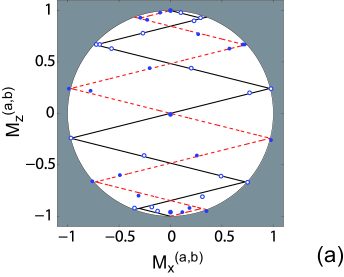
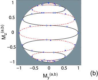
Figure 2: (Color Online) Projections of the optimal trajectories for the inversion of the two Bloch vectors with offsets, $\omega/2\pi=\pm 483$ Hz, in the $(x,z)$- and $(y,z)$- plane are shown in (a) and (b), respectively. The simulated trajectories of the two spins are plotted in black solid line and red dashed line. The experimentally measured trajectories of the two magnetization vectors are represented by open and filled circles.

5 Summary

In this last section, we give a brief overview of the results obtained in this paper. The four relevant cases for the simultaneous inversion of two spins are the following.

1. two control fields along the $x$- and $y$- directions and one offset $\omega$: the optimal solution is a $\pi$- pulse [8].

2. one control field and one offset $\omega$: the optimal solution is a bang-bang pulse sequence with a number of switching depending upon the ratio $\omega/\omega_{max}$ [9].

3. one control field and two offsets $\omega$ and $-\omega$: The optimal solution is the same as in (2).

4. two control fields and two offsets $\omega$ and $-\omega$: The optimal solution is also the same as in (2).

Aknowledgment.
S.J.G. acknowledges support from the DFG (GI 203/6-1), SFB 631. S. J. G. and M. B. thank the Fonds der Chemischen Industrie. Experiments were performed at the Bavarian NMR center at TU München and we thank Dr. R. Marx for helpful discussions and for suggesting the test sample.

References

- [1] M. H. Levitt, Spin dynamics: basics of nuclear magnetic resonance (John Wiley and sons, New York-London-Sydney, 2008); R. R. Ernst, G. Bodenhausen and A. Wokaun, Principles of Nuclear Magnetic Resonance in one and two dimensions (International Series of Monographs on Chemistry, Oxford University Press, Oxford, 1990)
- [2] L. M. K. Vandersypen and I. L. Chuang, Rev. Mod. Phys. 76, 1037 (2005); N. C. Nielsen, C. Kehlet, S. J. Glaser and N. Khaneja, in Encyclopedia of Magnetic Resonance, Ed. R. K. Harris and R. Wasylishen, John Wiley, Chichester (2010).
- [3] D. P. Frueh, T. Ito, J.-S. Li, G. Wagner, S. J. Glaser and N. Khaneja, J. Bio. NMR. 32, 23 (2005); J. L. Neves, B. Heitmann, N. Khaneja and S. J. Glaser, J. Magn. Reson. 201, 7 (2009).
- [4] D. G. Cory, A. F. Fahmy, and T. F. Havel, Proc. Natl. Acad. Sci. USA 94, 1634(1997); N.A. Gershenfeld and I.L. Chuang, Science 275, 350 (1997).
- [5] M. A. Nielsen and I. L. Chuang, Quantum Computation and Quantum Information (Cambridge University Press, Cambridge, 2000).
- [6] V. Jurdjevic, Geometric control theory (Cambridge University Press, Cambridge, 1996).
- [7] B. Bonnard and M. Chyba, Singular trajectories and their role in control theory (Springer SMAI, Vol. 40, 2003).
- [8] U. Boscain, G. Charlot, J.-P. Gauthier, S. Guérin and H. R. Jauslin, J. Math. Phys. 43, 2107 (2002)
- [9] U. Boscain and P. Mason, J. Math. Phys. 47, 062101 (2006).
- [10] U. Boscain and B. Piccoli, Optimal syntheses for control systems on 2-D manifolds, Mathématiques and Applications, 43, Springer-Verlag, Berlin, 2004.
- [11] A. E. Bryson and Y.-C. Ho, Applied Optimal Control, Taylon and Francis group, New-York-London, 1975.
- [12] N. Khaneja, R. Brockett and S. J. Glaser, Phys. Rev. A 63, 032308 (2001); N. Khaneja, S. J. Glaser and R. Brockett, Phys. Rev. A 65, 032301 (2002); H. Yuan and N. Khaneja, Phys. Rev. A 72, 040301(R) (2005)
- [13] M. Lapert, Y. Zhang, M. Braun, S. J. Glaser and D. Sugny, Phys. Rev. Lett. 104, 083001 (2010).
- [14] D. Sugny, C. Kontz and H.R. Jauslin, Phys. Rev. A 76, 023419 (2007); B. Bonnard and D. Sugny, SIAM J. on Control and Optimization, 48, 1289 (2009); B. Bonnard, M. Chyba and D. Sugny, IEEE Transactions on Automatic control, 54, 11, 2598 (2009)
- [15] T. E. Skinner, T. O. Reiss, B. Luy, N. Khaneja and S. J. Glaser, J. Magn. Reson. 163, 8 (2003); T. E. Skinner, T. O. Reiss, B. Luy, N. Khaneja and S. J. Glaser, J. Magn. Reson. 167, 68 (2004); K. Kobzar, T. E. Skinner, N. Khaneja, S. J. Glaser and B. Luy, J. Magn. Reson. 170, 236 (2004); T. E. Skinner, T. O. Reiss, B. Luy, N. Khaneja and S. J. Glaser, J. Magn. Reson. 172, 17 (2005); T. E. Skinner, K. Kobzar, B. Luy, R. Bendall, W. Bermel, N. Khaneja and S. J. Glaser, J. Magn. Reson. 179, 241 (2006); N. I. Gershenzon, K. Kobzar, B. Luy, S. J. Glaser and T. E. Skinner, J. Magn. Reson. 188, 330 (2007); K. Kobzar, T. E. Skinner, N. Khaneja, S. J. Glaser and B. Luy, J. Magn. Reson. 194, 58 (2008).
- [16] G. Turinici and H. Rabitz, Phys. Rev. A 70, 063412 (2004); H. Rabitz and G. Turinici, Phys. Rev. A 75, 043409 (2007); K. Sundermann, H. Rabitz and R. de Vivie-Riedle, Phys. Rev. A 62, 013409 (2000).
- [17] W. Zhu, J. Botina and H. Rabitz, J. Chem. Phys. 108, 1953 (1998); W. Zhu and H. Rabitz, J. Chem. Phys. 110, 7142 (1999); D. Sugny, C. Kontz, M. Ndong, Y. Justum, G. Dive and M. Desouter-Lecomte, Phys. Rev. A 74, 043419 (2006); D. Sugny, M. Ndong, D. Lauvergnat, Y. Justum and M. Desouter-Lecomte, J. Photochem. Photobiol. A 190, 359 (2007); M. Ndong, L. Bomble, D. Sugny, Y. Justum and M. Desouter-Lecomte, Phys. Rev. A 76, 043424 (2007).
- [18] Y. Chitour, F. Jean and E. Trélat, SIAM J. Control Optim. 47, 1078 (2008).