Vison excitations in near-critical quantum dimer models

Abstract

We study vison excitations in a quantum dimer model interpolating between the Rokhsar–Kivelson models on the square and triangular lattices. In the square-lattice case, the model is known to be critical and characterized by U(1) topological quantum numbers. Introducing diagonal dimers brings the model to a Z₂ resonating-valence-bond phase. We study variationally the emergence of vison excitations at low concentration of diagonal dimers, close to the critical point. We find that, in this regime, vison excitations are large in size and their structure resembles vortices in type-II superconductors.

I Introduction

The resonating-valence-bond (RVB) state is one of the most exciting proposals for strongly correlated phases in two dimensions. Of potential relevance to frustrated spin systems 1974FazekasAnderson ; 2005MisguichLhuillier and high-temperature superconductivity 1987Anderson ; 2004AndersonEtAl , it has evaded a direct identification in experiments and in studies of realistic models. However, a spinless analogue of the RVB phase can be systematically studied in quantum dimer models, where this phase is rigorously confirmed and accessible to a variety of analytic and numerical methods 2001MoessnerSondhiFradkin ; 2008MoessnerRaman . Furthermore, quantum dimer models have also motivated the construction of SU(2) invariant examples of RVB phases in spinful sytstems 2005RamanMoessnerSondhi ; 2005Fujimoto ; 2010CanoFendley .

The main strongly correlated feature of the RVB phase is the existence of fractionalized excitations. In a spin system, in the conjectured RVB phase, two types of elementary excitations must be present: spinons (spin-1/2 excitations) and visons (Z₂ vortices). They have relative semionic statistics: a $-1$ factor for an elementary braiding of a spinon around a vison 1987KivelsonRokhsarSethna ; 2001SenthilFisher . In dimer models, spinon excitations are absent (or effectively pushed to infinitely high energy), and only vison excitations and their combinations appear in the spectrum 2004Ivanov . Another consequence of the existence of vison excitations is the so called “topological order”: a degeneracy of the ground states (and low-lying excitations) for systems on multiply connected domains 1988RokhsarKivelson ; 1989ReadChakraborty .

An interesting question arises regarding the fate of these elementary excitations near phase transitions from the RVB phase to neighboring non-topological phases. Two generic phase transitions of this sort may be envisioned. Either singlets (or dimers in dimer models) order into a valence-bond-crystal, or spins order into some sort of magnetic order. These two possible paths for the RVB state were identified in Ref. 2006Ivanov, as two conditions for the topological order in Gutzwiller-projected wave functions. A field-theoretic model of these phase transitions has been proposed and analyzed in Ref. 2009XuSachdev, .

In the present paper, we consider another, non-generic phase transition into a U(1) critical state. This transition is most easily realized by deforming a model on a bipartite lattice (with U(1) winding numbers) into one on a non-bipartite lattice (with the U(1) symmetry broken down to Z₂). While this transition represents a non-generic, “fine-tuned” situation, it also allows for an analytic treatment of quantum dynamics near the critical point. Specifically, we consider an interpolation between the Rokhsar–Kivelson (RK) models on the square and triangular lattices in such a way that the exact solvability of the RK ground states is preserved throughout the interpolation.

In such a model, close to the critical point, we can variationally construct vison excitations, thus estimating the size of the vison gap and identifying the associated length scale (the vison size). We find that the vison gap closes at the transition point while the vison size diverges. The shape of the vison in this limit resembles vortices in type-II superconductors, with the vison size corresponding to the magnetic penetration length.

The paper is organized as follows. In Section II, we briefly review the properties of the RK dimer models on the square and triangular lattices. In Section III, we describe the interpolating model which connects those lattices. In Section IV, we construct variational vison excitations near the critical point and discuss their properties. Finally, in Section V we discuss some interesting aspects of our results.

II Rokhsar–Kivelson dimer models on square and triangular lattices

The Rokhsar–Kivelson dimer model on any lattice is defined in the Hilbert space of all fully packed coverings of the lattice by dimers by the Hamiltonian 1988RokhsarKivelson ; 2001MoessnerSondhi

$$H_{\rm RK}=\sum\Big{(}-t\left|\lower 2.15277pt\hbox{ \includegraphics[width=8.61108pt]{fig-hor.pdf}}\,\,\right\rangle\left\langle\lower 2.15277pt\hbox{ \includegraphics[width=8.61108pt]{fig-vert.pdf}}\,\,\right|+v\left|\lower 2.15277pt\hbox{ \includegraphics[width=8.61108pt]{fig-hor.pdf}}\,\,\right\rangle\left\langle\lower 2.15277pt\hbox{ \includegraphics[width=8.61108pt]{fig-hor.pdf}}\,\,\right|\Big{)}$$ (1)

where the sum is taken over all tetragonal plaquettes of the lattice. In the present work, we are interested in this model on the square and triangular lattices in two dimensions, in which cases the sums are understood as those over all the plaquettes of the square lattice and over all the two-plaquette rhombi of the triangular lattice, respectively.

On both lattices, there is a special case of the model (1) with $v=t$ (called the RK point), in which the ground state is exactly known and given by all the allowed dimer configurations with equal amplitudes 1988RokhsarKivelson ,

$$\left|{\rm GS}\right\rangle=\frac{1}{\sqrt{Z}}\sum_{c}\left|c\right\rangle$$ (2)

(here the sum is taken over all dimer configurations, and $Z$ is a normalization factor). However, the properties of this state and of the lowest excitations above it are very different in the cases of square and triangular lattices, due to the fact that one of them (square) is bipartite, and the other one (triangular) is not.

On the square (bipartite) lattice, the correlations are power-law 1963FisherStephenson and the spectrum is gapless: the elementary excitations are so called resonons with the dispersion $\omega(k)\propto k^{2}$ 1988RokhsarKivelson ; 1997Henley .

On the triangular (nonbipartite) lattice, the correlations decay exponentially with distance 2001MoessnerSondhi ; 2002FendleyMoessnerSondhi ; 2002IoselevichIvanovFeigelman , and the spectrum is gapped 2001MoessnerSondhi ; 2004Ivanov with two types of excitations. One sector of excitations is of the vison type (topological Z₂ vortices), and the other sector is formed by excitations local in terms of dimer operators (those excitations can be thought of as composed of an even number of vison excitations).

This difference between the physics of the RK states on bipartite and non-bipartite lattices can be traced down to a larger set of conserved quantities in bipartite dimer models. Namely, dimer configurations on bipartite lattices may be mapped onto a scalar height field 1990Levitov ; 1997Henley ; 2009NogueiraNussinov , whose winding numbers provide integer-valued topological invariants (in the dual variables, those integer winding numbers may be related to a U(1) gauge symmetry). On the other hand, on non-bipartite lattices, only a Z₂ subgroup of winding numbers survives, thus breaking the U(1) symmetry down to Z₂. The above difference between bipartite and non-bipartite lattices is well known and extensively discussed in literature, and we refer the reader to other studies for details 2001MoessnerSondhiFradkin ; 2000SachdevVojta ; 2008LaeuchliCapponiAssaad .

Figure 1: (a) The interpolated model is defined on the square lattice with links added along one of the diagonal directions. The dashed line connecting plaquettes $\alpha$ and $\beta$ illustrates the point-vison construction (7). (b)–(d) The three possible dimer-flip processes. The process (b) is contained in the “square” part of the Hamiltonian (4); the processes (c) and (d) are included in the “diagonal” part (5).

III Interpolation between the RK dimer models on square and triangular lattices

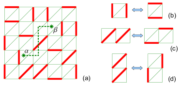
In our present work, we analyse an interpolation between the RK points on the square and triangular quantum lattices. We introduce this interpolation in such a way that the “RK solvability” for the ground state is preserved in the interpolating model. Namely, we construct the interpolation by introducing dimers along one of the diagonal directions of the plaquettes of the square lattice (Fig. 1a). Then by tuning the fugacity of diagonal dimers, one can interpolate between the two limiting cases of the square and triangular lattices.

The Hamiltonian of the interpolating model is thus chosen to be

$$H=H_{\rm square}+H_{\rm diag}\,,$$ (3)

where

$$H_{\rm square}=\sum\Big{(}|\lower 1.93747pt\hbox{ \includegraphics[width=8.61108pt]{fig-square1.pdf}}\,\,\rangle-|\lower 1.93747pt\hbox{ \includegraphics[width=8.61108pt]{fig-square2.pdf}}\,\,\rangle\Big{)}\Big{(}\langle\lower 1.93747pt\hbox{ \includegraphics[width=8.61108pt]{fig-square1.pdf}}\,\,|-\langle\lower 1.93747pt\hbox{ \includegraphics[width=8.61108pt]{fig-square2.pdf}}\,\,|\Big{)}$$ (4)

is the RK Hamiltonian (1) on the square lattice with $v=t=1$ (involving kinetic and potential processes for square plaquettes depicted in Fig. 1b) and

$$H_{\rm diag}=\kappa\sum\Big{(}|\lower 1.93747pt\hbox{ \includegraphics[width=17.22217pt]{fig-diag1.pdf}}\,\,\rangle-\mu|\lower 1.93747pt\hbox{ \includegraphics[width=17.22217pt]{fig-diag2.pdf}}\,\,\rangle\Big{)}\Big{(}\langle\lower 1.93747pt\hbox{ \includegraphics[width=17.22217pt]{fig-diag1.pdf}}\,\,|-\mu\langle\lower 1.93747pt\hbox{ \includegraphics[width=17.22217pt]{fig-diag2.pdf}}\,\,|\Big{)}$$ (5)

is the term involving diagonal dimers. The sum is taken over two types of parallelogram plaquettes depicted in panels c and d of Fig. 1. The ground state of this Hamiltonian is then

$$\left|{\rm GS}\right\rangle=\frac{1}{\sqrt{Z}}\sum_{c}\mu^{D(c)/2}\left|c\right\rangle\,,$$ (6)

where $D(c)$ is the number of diagonals in a given configuration $c$.

Note that this is a two-parameter interpolation: the parameter $\mu$ is responsible for the ground state of the Hamiltonian, while the parameter $\kappa$ determines the dynamics of diagonal dimers. At $\mu=\kappa=0$, the Hamiltonian reduces to the RK point on the square lattice, while $\mu=\kappa=1$ reproduces the RK point on the isotropic triangular lattice.

The above model was introduced in Ref. 2006Perseguers, , where a simple variational ansatz for the excitations was proposed. The properties of the ground state (6) were analyzed in the earlier work Ref. 2002FendleyMoessnerSondhi, . From the Pfaffian technique 1963Kasteleyn , one easily deduces the ground-state correlation length $\xi\propto\mu^{-1}$. One can expect that at any nonvanishing $\mu$ and $\kappa$, the system belongs to the Z₂ phase with excitations continuously connected to those on the isotropic triangular lattice. This scenario has also been proposed in Refs. 2001MoessnerSondhiFradkin, and 2000SachdevVojta, on the basis of a field-theoretical analysis: such an interpolation can be interpreted as a U(1) gauge theory coupled to a charge-two scalar field. In the present paper, we complement this general analysis with a microscopic construction of vison excitations in the interpolating model (3)–(5) close to the critical point (for small deformation parameters $\mu$ and $\kappa$).

In Ref. 2006Perseguers, , variational constructions for dimer (resonon) and vison excitations have been proposed. For the resonon excitations, a quasi-perturbative construction gives a gap $\Delta_{\rm dim}\propto\mu^{2}\kappa$ (which is likely to be an exact asymptotic behavior of the dimer gap in our model). At the same time, an attempt to construct variational vison excitations as plane waves of point visons proposed in Ref. 2006Perseguers, produced states with a finite variational energy that does not tend to zero in the limit of the square lattice ($\mu,\kappa\to 0$). This suggests (and we will confirm it in the next section) that point visons are not good variational states, but the actual vison eigenstates extends over many lattice spacings (in the limit $\mu,\kappa\to 0$). The following section is devoted to constructing such states.

IV Variational construction of vison excitations

To construct variational visons, we first define point visons and then dress them with local operators to approximate eigenstates. To define visons, one takes a contour $\Gamma_{\alpha\beta}$ connecting two plaquettes $\alpha$ and $\beta$ of the lattice and considers the intersection-parity operator (Fig. 1) 1989ReadChakraborty ,

$$V_{\alpha\beta}=(-1)^{{\rm number~{}of~{}dimers~{}intersecting~{}}\Gamma_{\alpha\beta}}\,.$$ (7)

One easily verifies (i) that this operator is independent of the contour $\Gamma_{\alpha\beta}$ connecting two given points, up to an overall controlled change of sign; (ii) that the commutator of $V_{\alpha\beta}$ with any local dimer Hamiltonian is concentrated near the points $\alpha$ and $\beta$; and (iii) that $V_{\alpha\beta}V_{\beta\gamma}=V_{\alpha\gamma}$. Therefore one can decompose the operator $V_{\alpha\beta}$ into the product of two vison operators, which have the structure of Z₂ vortices 2004Ivanov ,

$$V_{\alpha\beta}=V_{\alpha}V_{\beta}\,.$$ (8)

Alternatively, one can understand the operator $V_{\alpha}$ as the parity operator (7) with the point $\beta$ sent to infinity.

Such a point-vison operator produces a state orthogonal to the original state, but not an eigenstate. To form an eigenstate (or, more precisely, a wave packet of lowest-energy eigenstates), one needs to dress a point vison,

$$\left|{\rm V}\right\rangle=\hat{D}\,V_{\alpha}\left|{\rm GS}\right\rangle$$ (9)

where $\hat{D}$ is some operator local in terms of dimers.

We may suggest (and this suggestion is further confirmed by a variational calculation) that, in order to lower the variational energy, we should spread the vison flux from one plaquette to a certain region of the lattice. On the square lattice, the point vison may be written in terms of the height field as

$$V_{\alpha}=\exp(iKh_{\alpha})$$ (10)

where $K$ is some constant depending on the normalization convention for the height field $h_{\alpha}$. The spreading of the vison flux can then be achieved by the dressing operator

$$\hat{D}=\exp\left[i\sum_{\beta}f_{\beta}(h_{\beta}-h_{\alpha})\right]$$ (11)

with some weights $f_{\beta}$ determining the flux redistribution. We will further use another expression equivalent to Eq. (11) on the square lattice, but also directly generalizable to the interpolating model (where the height field $h_{\alpha}$ is no longer defined). Namely, we use the following variational ansatz:

$$\hat{D}=\exp\left[i\sum_{\langle jk\rangle}\tilde{A}_{jk}n_{jk}\right]\,,$$ (12)

where the sum is taken over all lattice links and $n_{jk}$ is the dimer density on the link $\langle jk\rangle$ (equal to 1 or 0 in the presence/absence of a dimer, respectively). Thus constructed variational state has a gauge redundancy: a transformation

$$\tilde{A}_{jk}\mapsto\tilde{A}_{jk}+\varphi_{j}+\varphi_{k}$$ (13)

does not change the state (9), up to an overall phase. Therefore, without loss of generality, we may put $\tilde{A}_{jk}=0$ on all diagonal links and thereby fix the gauge. Finally, it will be convenient to convert $\tilde{A}_{jk}$ (defined now on the square lattice) into a vector potential $A_{jk}$ by

$$A_{jk}=(-1)^{j}\tilde{A}_{jk}$$ (14)

The variational energy of the “square” part of the Hamiltonian (4) in the state (9), (12) is given by

$$E_{\rm square}=\left\langle{\rm V}\right|H_{\rm square}\left|{\rm V}\right\rangle=P_{\rm flip}^{(1)}\sum_{\beta}(1-\cos\phi_{\beta})$$ (15)

where $P_{\rm flip}^{(1)}$ is the probability of a given square plaquette to be flippable (at the RK point on the square lattice, $P_{\rm flip}^{(1)}=1/4$) 2006Perseguers and $\phi_{\beta}$ is the flux at the plaquette $\beta$. This flux is composed of the flux of the vector potential $A_{jk}$ and of the flux of the original point vison $V_{\alpha}$ in Eq. (9):

$$\phi_{\beta}=A_{12}+A_{23}+A_{34}+A_{41}+\pi\delta_{\alpha\beta}\,,$$ (16)

where the numerical indices 1 to 4 label the four sites of the square plaquette $\beta$ in the cyclic order. Since we assume that the operator $\hat{D}$ is local in terms of dimers and concentrated in a finite region near the plaquette $\alpha$, the total flux of the vector potential $A_{jk}$ must vanish. Therefore, we find the constraint for the total flux $\phi_{\beta}$,

$$\sum_{\beta}\phi_{\beta}=\pi\,.$$ (17)

On the square lattice (at $\mu=\kappa=0$), the total variational energy is given by Eq. (15). Its minimization with the constraint (17) yields the spreading of the flux over the whole lattice. Indeed, spreading the flux over $N$ plaquettes gives $N$ fluxes $\phi_{\beta}\propto 1/N$, which results in the total energy $E\propto 1/N$. This variational construction shows that, indeed, in the limit of the square lattice the vison excitation becomes unstable and that close to the critical point the vison size must be large (much larger than the lattice spacing). In this limit, using the fact that the optimal fluxes $\phi_{\beta}$ are small, we can expand the cosine in Eq. (15) and write the long-wavelength expression for the energy,

$$E_{\rm square}=\frac{P_{\rm flip}^{(1)}}{2}\int(\vec{\nabla}\times\vec{A})^{2}\,d^{2}x\,.$$ (18)

with the total screened flux

$$\oint_{x_{\alpha}}\vec{A}\,d\vec{x}=\pi$$ (19)

[the latter integral is taken over a small circle surrounding the position $x_{\alpha}$ of the point vison in Eq. (9); this point is excluded from the integral (18)].

In the interpolating model (at finite $\mu$ and $\kappa$), the second term in the Hamiltonian (5) stabilizes the vison. Indeed, its contribution for our variational state (9), (12) can be written, in the long-wavelength limit, as

$$E_{\rm diag}=4\kappa\mu^{2}P_{\rm flip}^{(2)}\int\vec{A}^{2}\,d^{2}x\,.$$ (20)

Here we assume that the vector potential $\vec{A}$ is small and slowly varying on the length scale of one lattice constant. This is a valid assumption far from the vison center. The central region gives a contribution of the order $\kappa\mu^{2}$ to the vison energy, which can be neglected to the leading order, in comparison with the logarithmically larger contribution from large distances. The coefficient $P_{\rm flip}^{(2)}$ is given by the probability to find two parallel non-diagonal dimers on a “skew” (parallelogram) plaquette. To the leading order in $\mu$, it can be approximated by its value at the RK point on the square lattice, $P_{\rm flip}^{(2)}\approx 0.04542$ 2006Perseguers . The total variational energy of the vison can now be written as

$$E=E_{\rm square}+E_{\rm diag}=\frac{P^{(1)}_{\rm flip}}{2}\int d^{2}x\,\left[(\vec{\nabla}\times\vec{A})^{2}+\frac{1}{L^{2}}\vec{A}^{2}\right]\,,$$ (21)

where the new large length scale (“size of vison”) emerges,

$$L=\sqrt{\frac{P^{(1)}_{\rm flip}}{8P^{(2)}_{\rm flip}}}\cdot\kappa^{-1/2}\mu^{-1}\,.$$ (22)

Remarkably, this variational problem is equivalent to that of a vortex in a type-II superconductor (with $L$ corresponding to the London penetration length) 1996Tinkham . In terms of the “magnetic field” defined as

$$B=\vec{\nabla}\times\vec{A}\,,$$ (23)

the variational problem (21) is equivalent to minimizing the energy

$$E=\frac{P^{(1)}_{\rm flip}}{2}\int d^{2}x\,\left[B^{2}+L^{2}\left(\vec{\nabla}\times B\right)^{2}\right]\,,$$ (24)

with the total-flux constraint

$$\int B\,d^{2}x=\pi\,.$$ (25)

One can find a centrally-symmetric solution to this variational problem,

$$B(R)=\frac{1}{2L^{2}}K_{0}\left(\frac{R}{L}\right)\,,$$ (26)

where $K_{0}$ is the modified Bessel (Macdonald) function and $R$ is the distance from the vison center. The energy corresponding to this solution is

$$E=\frac{\pi P^{(1)}_{\rm flip}}{4L^{2}}\ln L=-\pi P^{(2)}_{\rm flip}\kappa\mu^{2}\ln(\kappa\mu^{2})\,.$$ (27)

Of course, this result for the energy, as well as the long-wavelength approximation (18) – (21) and (24) – (26), is only justified if $L\gg 1$. The expression (26) for the variational solution is also only valid for $R\gg 1$.

V Discussion of results

In the preceding section, we have constructed a variational vison excitation in a near-critical RK-type dimer model interpolating between the RK points on the square and triangular lattices. While, rigorously speaking, our construction provides an upper bound for the gap in the vison excitation sector, we believe that it captures the main qualitative feature of vison excitations (spreading the vison flux over a large region of lattice), and therefore conjecture that it also gives the exact functional dependence on the deformation parameters $\mu$ and $\kappa$. Below we discuss several interesting aspects and implications of our result.

First of all, our variational construction is only based on the large length scale $L\gg 1$, which is equivalent to $\kappa\mu^{2}\ll 1$. Thus we do not, in fact, require the individual smallness of the parameters $\kappa$ and $\mu$, but only of their above combination.

Second, we find that the (variational) vison gap closes as

$$E_{\rm vison}\propto\frac{1}{L^{2}}\ln L$$ (28)

at the critical point. This behavior should be compared to the variational analysis of the dimer gap in the same model performed in Ref. 2006Perseguers, . There it was found that the dimer gap closes as

$$E_{\rm dimer}\propto\frac{1}{L^{2}}\,,$$ (29)

i.e., it is always smaller close to the critical point. This suggests that visons tend to form bound pairs thus canceling the logarithmic term in the energy (see also the discussion of two vison signs below).

Third, our variational vison can have two different signs, which correspond to the two opposite signs of the smeared flux $B$. While there is only one species of the point vison (fluxes $\pi$ and $-\pi$ on one plaquette are identical), there is a freedom of smearing this flux as either positive or negative over many plaquettes (of course, there are also options to smear fluxes $\pm 3\pi$, $\pm 5\pi$, etc., but they are obviously higher in energy). As a result, we can construct two variational visons differing by the sign of the field $B$. This result may appear surprising in view of our expectation of the Z₂ structure of vison excitations. This paradox can be resolved by analysing the properties of our variational visons with respect to the translational symmetries.

Figure 2: (a) The two elementary translations of the lattice, which anticommute for vison states. (b) The $k$ space for vison excitations. The labeling of the points $A$, $B$, and $C$ is the same as in the isotropic triangular lattice case considered in Ref. 2004Ivanov, (see Fig. 3 there). In our interpolating model, points $C_{1}$ and $C_{2}$ are not degenerate: they only become degenerate in the triangular lattice limit ($\kappa=\mu=1$). Close to the critical point (square lattice), the vison minima are located at points $C_{1}$. Note that the vison Brillouin zone is only one half of the usual dimer Brillouin zone, and therefore it contains two $C_{1}$ points.

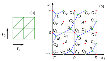
As follows from their construction, visons live on a frustrated lattice 2001MoessnerSondhiFradkin ; 2004Ivanov . In terms of translational symmetries, this implies that the elementary translations in the $x_{1}$ and $x_{2}$ directions (along the links of the square lattice, Fig. 2a) anticommute:

$$T_{1}T_{2}=-T_{2}T_{1}$$ (30)

Therefore, to define a wave vector for vison eigenstates, one needs to double the unit cell. In terms of $k$ vectors, this implies the period of $\pi$ in the directions $k_{1}$ and $k_{2}$ for the dispersion relation. More precisely, to the four $k$ points $(k_{1},k_{2})$, $(k_{1}+\pi,k_{2})$, $(k_{1},k_{2}+\pi)$, and $(k_{1}+\pi,k_{2}+\pi)$, there correspond two linearly independent vison eigenstates degenerate in energy.

By analyzing the action of the translation operators on our variational vison states, we conclude that these states belong to the vicinity of the wave vectors generated by $k=(0,0)$. Thus the two vison states of opposite fluxes correspond to the two degenerate minima of the vison dispersion relation. Extending the notation of Ref. 2004Ivanov, , these minima can be denoted as $C_{1}$ (which become degenerate with points $C_{2}$ in the isotropic triangular limit, see Fig. 2b). Note that these points are different from the energy minima on the isotropic triangular lattice ($\kappa=\mu=1$), which are located at points $B$ 2004Ivanov .

Remarkably, the existence of visons of opposite signs can qualitatively explain the formation of vison bound states (dimer-like excitations) found numerically in Ref. 2004Ivanov, . Indeed, superimposing visons of opposite signs at a short distance (much shorter than $L$) compensates the long-distance logarithmic contribution to the energy (28), thus producing the energy of the bound state (29).

Fourth, an analogy with type-II superconductors can be drawn not only in the variational form of the energy (21) or (24), but also in the existence of two different length scales. The vison size $L$ in our problem obviously corresponds to the London penetration length in the theory of superconductivity. On the other hand, there is a second length scale $\xi$ (the ground-state correlation length), which resembles the superconducting coherence length. In superconductors, the interplay of the two length scales leads to important physical consequences (difference between type-I and type-II superconductors). We may therefore conjecture that in quantum dimer models some novel effects depending on the relation between the two lengths may also be possible. Note, however, that this analogy is not complete: in our vison construction, the length scale $\xi$ does not enter, and only the length $L$ affects the variational state and its energy. In fact, the lower cut-off of the logarithm in the vison energy (28) is given by the lattice spacing rather then $\xi$. It would be interesting to explore further improvements of our variational ansatz, which may bring in the length scale $\xi$ (by analogy to the core of superconducting vortices). We leave this interesting question for future study.

Another interesting question that remains unexplored is the dynamics of visons in our model. While exact vison eigenstates must carry a well-defined wave vector $k$, our variational state is localized in space and thus corresponds to a wave packet of width $\Delta k\sim 1/L\ll 1$ in the reciprocal space. We believe that its energy accurately represents the bottom of the vison band, but the question of the vison mass remains unresolved in our construction.

While the study reported in the present paper relates to a very specific model and to a non-generic phase transition between a RVB phase and a U(1) critical point, we believe that some of our findings may be generalized to other systems and situations. In particular, the existence of two different length scales ($\xi$ and $L$) is likely to be a general property of the RVB phase. The divergence of the vison size may also occur at other types of second-order phase transitions. We therefore hope that the example considered in the present paper will provide a guidance for future studies of the RVB phase in various systems and models.

We are grateful to G. Blatter, M. Feigelman, R. Moessner, D. Poilblanc, and D. Sadri for helpful discussions and comments on this work.

References

- (1) P. Fazekas and P. W. Anderson, Philos. Mag. 30, 423 (1974).
- (2) G. Misguich and C. Lhuillier, in Frustrated spin systems, ed. H. T. Diep (World-Scientific, Singapore 2005).
- (3) P. W. Anderson, Science 235, 1196 (1987).
- (4) P. W. Anderson et al, J. Phys. Cond. Matt. 16, R755 (2004).
- (5) R. Moessner, S. L. Sondhi, and E. Fradkin, Phys. Rev. B 65, 024504 (2001).
- (6) R. Moessner and K. S. Raman, e-print arXiv:0809.3051 (2008) [lecture notes, Trieste 2007].
- (7) K. S. Raman, R. Moessner, and S. L. Sondhi, Phys. Rev. B 72, 064413 (2005).
- (8) S. Fujimoto, Phys. Rev. B 72, 024429 (2005).
- (9) J. Cano and P. Fendley, Phys. Rev. Lett. 105, 067205 (2010).
- (10) S. A. Kivelson, D. S. Rokhsar, and J. P. Sethna, Phys. Rev. B 35, 8865 (1987).
- (11) T. Senthil and M. P. A. Fisher, Phys. Rev. B 62, 7850 (2000); ibid. 63, 134521 (2001).
- (12) D. S. Rokhsar and S. A. Kivelson, Phys. Rev. Lett. 61, 2376 (1988).
- (13) P. Fendley, R. Moessner, and S. L. Sondhi, Phys. Rev. B 66, 214513 (2002).
- (14) D. A. Ivanov, Phys. Rev. B 70, 094430 (2004).
- (15) N. Read and B. Chakraborty, Phys. Rev. B 40, 7133 (1989).
- (16) D. A. Ivanov, Phys. Rev. B 74, 024525 (2006).
- (17) C. Xu and S. Sachdev, Phys. Rev. B 79, 064405 (2009).
- (18) R. Moessner and S. L. Sondhi, Phys. Rev. Lett. 86, 1881 (2001).
- (19) M. E. Fisher and J. Stephenson, Phys. Rev. 132, 1411 (1963).
- (20) C. L. Henley, J. Stat. Phys. 89, 483 (1997).
- (21) A. Ioselevich, D. A. Ivanov, and M. V. Feigelman, Phys. Rev. B 66, 174405 (2002).
- (22) L. S. Levitov, Phys. Rev. Lett. 64, 92 (1990).
- (23) F. S. Nogueira and Z. Nussinov, Phys. Rev. B 80, 104413 (2009).
- (24) S. Sachdev and M. Vojta, J. Phys. Soc. Jap. 69, Suppl. B, 1 (2000) [cond-mat/9910231].
- (25) A. Laeuchli, S. Capponi, and F. F. Assaad, J. Stat. Mech. P01010 (2008).
- (26) S. Perseguers, Master thesis, EPFL, Lausanne (2006).
- (27) P. W. Kasteleyn, J. Math. Phys. 4, 287 (1963); S. Samuel, ibid. 21, 2806 (1980).
- (28) N. Read and S. Sachdev, Phys. Rev. Lett. 66, 1773 (1991); S. Sachdev, arXiv:1002.3823.
- (29) D. Ivanov and T. Senthil, Phys. Rev. B 66, 115111 (2002).
- (30) M. Tinkham, Introduction to superconductivity, 2nd ed., McGraw-Hill, New York (1996).