Integrated Markov Chain Monte Carlo (MCMC) analysis of primordial non-Gaussianity ($f_{\mathrm{NL}}$) in the recent CMB data

Abstract:

We have made a Markov Chain Monte Carlo (MCMC) analysis of primordial non-Gaussianity ($f_{\mathrm{NL}}$) using the WMAP bispectrum and power spectrum. In our analysis, we have simultaneously constrained $f_{\mathrm{NL}}$ and cosmological parameters so that the uncertainties of cosmological parameters can properly propagate into the $f_{\mathrm{NL}}$ estimation. Investigating the parameter likelihoods deduced from MCMC samples, we find slight deviation from Gaussian shape, which makes a Fisher matrix estimation less accurate. Therefore, we have estimated the confidence interval of $f_{\mathrm{NL}}$ by exploring the parameter likelihood without using the Fisher matrix. We find that the best-fit values of our analysis make a good agreement with other results, but the confidence interval is slightly different.

1 Introduction

Over the past years, there have been great successes in measurement of the CMB anisotropy by ground and satellite observations [1, 2, 3, 4, 5]. CMB anisotropy, which is associated with the inhomogeneity of the last scattering surface, provides invaluable information on our Universe. In particular, the angular power spectrum of CMB anisotropy provides strong constraints on cosmological models and cosmological parameters [6, 7, 8].

Large classes of cosmological inflation models predict some level of primordial non-Gaussianity ($f_{\mathrm{NL}}$), whose detailed shape and amplitude depend on the particular class of the inflationary model [9, 10, 11]. Therefore, an investigation of the imprints of primordial non-Gaussianity allows us to constrain and rule out some classes of inflationary models [12, 10, 11]. Since the release of the COBE and subsequently WMAP data [13, 14, 15, 16, 17, 1], there have been active investigations on the imprints of primordial non-Gaussianity, using CMB data from the satellite and sub-orbital experiments [18, 16, 19, 20, 21, 22, 23, 24, 25, 26, 27, 28, 29, 11]. Currently, the strongest limit is imposed on the local-type $f_{\mathrm{NL}}=32\pm 21$ by the WMAP data [28, 11]. CMB bispectrum, which is most sensitive to $f_{\mathrm{NL}}$ parameters, also have some dependence on cosmological parameters [9, 19, 11]. Noting this, we have simultaneously constrained $f_{\mathrm{NL}}$ and cosmological parameters by using the WMAP bispectrum and power spectrum. In this way, we have allowed the uncertainties of cosmological parameters to properly propagate to the $f_{\mathrm{NL}}$ estimation. The parameter likelihoods deduced from MCMC samples show slight deviation from Gaussian shape, which makes Fisher matrix estimation less accurate. Therefore, we have estimated the confidence intervals of $f_{\mathrm{NL}}$ by fully exploring the parameter likelihood without using Fisher matrix. We find our estimation makes a good agreement with the existing results, but the confidence interval of $f_{\mathrm{NL}}$ is slightly different.

The outline of this paper is as follows. In Section 2, we discuss the primordial non-Gaussianity. In Section 3 and 4, we discuss the CMB bispectrum and its likelihood function. In Section 5, we make an analysis of WMAP data and present the results. In Section 6, we summarize our analysis and discuss prospects.

2 Primordial perturbations

Primordial perturbation in Fourier space is given by [30, 9, 31, 22]:

$$\Phi(\mathbf{k})=\Phi_{\mathrm{L}}(\mathbf{k})+\Phi_{\mathrm{NL}}(\mathbf{k}),$$ (1)

where $\Phi_{\mathrm{L}}(\mathbf{k})$ and $\Phi_{\mathrm{NL}}(\mathbf{k})$ denote the primordial perturbation of purely Gaussian nature and the deviation respectively. In most of inflationary models, $\Phi_{\mathrm{L}}(\mathbf{k})$, which follows a Gaussian distribution and statistical isotropy, have the following statistical properties [6, 7, 8]:

$$\langle\Phi_{\mathrm{L}}(\mathbf{k}_{1})\Phi_{\mathrm{L}}(\mathbf{k}_{2})\rangle = (2\pi)^{3}P_{\Phi}(k)\,\delta(\mathbf{k}_{1}+\mathbf{k}_{2}),$$ (2)

where $\langle\ldots\rangle$ denotes the average over an ensemble of universes, and $P_{\Phi}(k)=A\,k^{n-4}$ is a primordial power spectrum with a normalization amplitude $A$. The non-Gaussian part of the primordial perturbation, $\Phi_{\mathrm{NL}}(\mathbf{k})$, has negligible 2-point correlation [32, 12], which is also severely constrained by observational data:

$$\langle\Phi_{\mathrm{NL}}(\mathbf{k}_{1})\Phi_{\mathrm{NL}}(\mathbf{k}_{2})\rangle \approx 0.$$ (3)

Additionally, we may consider a 3-point correlation. For Gaussian $\Phi_{\mathrm{L}}(\mathbf{k})$, we expect a vanishing 3-point correlation [6, 7, 8, 9]:

$$\langle\Phi_{\mathrm{L}}(\mathbf{k}_{1})\,\Phi_{\mathrm{L}}(\mathbf{k}_{2})\,\Phi_{\mathrm{L}}(\mathbf{k}_{3})\rangle=0.$$ (4)

On the other hand, a non-vanishing 3-point correlation of $\Phi_{\mathrm{NL}}(\mathbf{k})$ is predicted by large classes of inflationary models:

$$\langle\Phi_{\mathrm{NL}}(\mathbf{k}_{1})\,\Phi_{\mathrm{NL}}(\mathbf{k}_{2})\,\Phi_{\mathrm{NL}}(\mathbf{k}_{3})\rangle=(2\pi)^{3}\delta(\mathbf{k}_{1}+\mathbf{k}_{2}+\mathbf{k}_{3})\,F(k_{1},k_{2},k_{3}).$$ (5)

where $F(k_{1},k_{2},k_{3})$ denotes a primordial bispectrum, whose detailed shape depends on the specific inflationary model [10]. In this paper, we shall consider the “local” and “equilateral” forms of the bispectrum, which are respectively associated with the squeezed and equilateral configuration of three vectors [30, 9, 31, 10, 33, 22, 34, 28, 11]. The primordial bispectrum in its “local” and “equilateral” forms is defined as follows [10, 35, 11]:

$$F_{\mathrm{local}}(k_{1},k_{2},k_{3}) = 2A^{2}f^{\mathrm{local}}_{\mathrm{NL}}\left[\frac{1}{k^{4-n}_{1}k^{4-n}_{2}}+\frac{1}{k^{4-n}_{2}k^{4-n}_{3}}+\frac{1}{k^{4-n}_{3}k^{4-n}_{1}}\right],$$

$$F_{\mathrm{equil}}(k_{1},k_{2},k_{3}) = 6A^{2}f^{\mathrm{equil}}_{\mathrm{NL}}\left[-\frac{1}{k^{4-n}_{1}k^{4-n}_{2}}-\frac{1}{k^{4-n}_{2}k^{4-n}_{3}}-\frac{1}{k^{4-n}_{3}k^{4-n}_{1}}-\frac{2}{(k_{1}k_{2}k_{3})^{2(4-n)/3}}\right.$$

$$\left.+\left(\frac{1}{k^{(4-n)/3}_{1}k^{2(4-n)/3}_{2}k^{4-n}_{3}}+(\mathrm{5\>perm.})\right)\right],$$

where $f^{\mathrm{local}}_{\mathrm{NL}}$ and $f^{\mathrm{equil}}_{\mathrm{NL}}$ denote the non-linear coupling parameters for “local” and “equilateral” forms respectively. The “local” form possesses a special significance because all single-field inflation models predict a negligible $f^{\mathrm{local}}_{\mathrm{NL}}$. Therefore, the detection of a high $f^{\mathrm{local}}_{\mathrm{NL}}$ would allow us immediately to rule out single-field inflation models [36, 37, 38, 39, 11]. Besides the aforementioned forms, there are also other forms for primordial bispectrum, which are predicted by certain inflation models [40, 41, 42, 43]. Therefore, the physical observables associated with the 3-point correlation provides important information on our early Universe.

3 The CMB anisotropy

The CMB anisotropy over a whole-sky is conveniently decomposed in terms of spherical harmonics:

$$T(\hat{\mathbf{n}}) = \sum_{lm}a_{lm}\,Y_{lm}(\hat{\mathbf{n}}),$$

where $a_{lm}$ and $Y_{lm}(\hat{\mathbf{k}})$ are a decomposition coefficient and a spherical harmonic function. The decomposition coefficient $a_{lm}$ is related to the primordial perturbations $\Phi(\mathbf{k})$ according to:

$$a_{lm} = 4\pi(-\imath)^{l}\int\frac{d^{3}\mathbf{k}}{(2\pi)^{3}}\Phi(\mathbf{k})\,g_{l}(k)\,Y^{*}_{lm}(\hat{\mathbf{k}}),$$ (6)

where $g_{l}(k)$ is a radiation transfer function. Largely, we may consider CMB power spectrum and bispectrum, which are associated with 2-point and 3-point correlation of primordial perturbation respectively. In the absence of tensor perturbation, the expectation value of CMB power spectrum is given by:

$$C_{l} = \langle a_{lm}\,a^{*}_{lm}\rangle$$ (7)

$$= \frac{2}{\pi}\int k^{2}dkg^{2}_{l}(k)\,P_{\Phi}(k).$$ (8)

As shown in Eq. 3, 2-point correlation of $\Phi_{\mathrm{NL}}(\mathbf{k})$ is insignificant. Therefore, the CMB power spectrum is mainly associated with $\Phi_{\mathrm{L}}(\mathbf{k})$ [32, 12] (c.f. Eq. 2).

Considering the rotational properties of spherical harmonics, we can construct a rotationally invariant estimator of the CMB bispectrum as follows [44]:

$$B^{\mathrm{obs}}_{l_{1}l_{2}l_{3}}=\sum_{m_{1}m_{2}m_{3}}\left(\begin{array}[]{ccc}l_{1}&l_{2}&l_{3}\\ m_{1}&m_{2}&m_{3}\end{array}\right)a_{l_{1}m_{1}}a_{l_{2}m_{2}}a_{l_{3}m_{3}}.$$ (11)

Hereafter, the condition ($l_{1}\leq l_{2}\leq l_{3}$) will be implied, unless stated otherwise. The expectation value of the CMB bispectrum, in other words, the theoretical CMB bispectrum, can be split into quantities associated with the different possible shapes of primordial non-Gaussianity:

$$\langle B^{\mathrm{obs}}_{l_{1}l_{2}l_{3}}\rangle=\sum_{\alpha}f^{i}_{\mathrm{NL}}\,B^{i}_{l_{1}l_{2}l_{3}},$$

where $i$ denotes “local” and “equilateral” in our analysis. The CMB bispectrum of $f^{i}_{\mathrm{NL}}=1$ is given by [9, 34, 22, 28, 11]:

$$B^{\mathrm{local}}_{l_{1}l_{2}l_{3}} = 2I_{l_{1}l_{2}l_{3}}\int^{\infty}_{0}r^{2}dr\left[\alpha_{l_{1}}(r)\beta_{l_{2}}(r)\beta_{l_{3}}(r)+\mathrm{2\>perm.}\right],$$ (12)

$$B^{\mathrm{equil}}_{l_{1}l_{2}l_{3}} = -3B^{\mathrm{local}}_{l_{1}l_{2}l_{3}}+6\,I_{l_{1}l_{2}l_{3}}\int^{\infty}_{0}r^{2}dr\left[\beta_{l_{1}}(r)\gamma_{l_{2}}(r)\delta_{l_{3}}(r)+(\mathrm{5\>perm.})-2\delta_{l_{1}}(r)\delta_{l_{2}}(r)\delta_{l_{3}}(r)\right],$$

where “perm.” denotes cyclic permutation and

$$I_{l_{1}l_{2}l_{3}}=\sqrt{\frac{(2l_{1}+1)(2l_{2}+1)(2l_{3}+1)}{4\pi}}\left(\begin{array}[]{ccc}l_{1}&l_{2}&l_{3}\\ 0&0&0\end{array}\right),$$ (16)

$$\alpha_{l}(r) = \frac{2}{\pi}\int k^{2}dk\,g_{Tl}(k)\,j_{l}(kr),$$ (17)

$$\beta_{l}(r) = \frac{2}{\pi}\int k^{2}dkP_{\Phi}(k)\,g_{Tl}(k)\,j_{l}(kr),$$ (18)

$$\gamma_{l}(r) = \frac{2}{\pi}\int k^{2}dkP^{1/3}_{\Phi}(k)\,g_{Tl}(k)\,j_{l}(kr),$$ (19)

$$\delta_{l}(r) = \frac{2}{\pi}\int k^{2}dkP^{2/3}_{\Phi}(k)\,g_{Tl}(k)\,j_{l}(kr),$$ (20)

with $j_{l}(x)$ being a spherical Bessel function. In our analysis, we have computed Eq. 12 and LABEL:B_equil by numerical integration. We have investigated the functional shape of the integrand and used 10, 10, 100 and 30 integration points for the intervals $r\leq 6.5$, $6.5<r\leq 13$, $13<r\leq 16.5$ and $16.5<r\leq 39.5$ [Gpc] respectively. Compared with a much denser sampling ($\times 50$), we find that the difference in the estimation of $f^{\mathrm{local}}_{\mathrm{NL}}$ is less than $1\%$. For $k$ space integration in Eq. 17, 18, 19 and 20, we used the $k$ space sampling of CAMB [45]. As discussed in Eq. 4, 3-point correlation of $\Phi_{\mathrm{L}}(\mathbf{k})$ is expected to be zero. Therefore, CMB bispectrum is not associated with $\Phi_{\mathrm{L}}(\mathbf{k})$, but only with $\Phi_{\mathrm{NL}}(\mathbf{k})$ (c.f. Eq. 5).

Due to foreground contamination, CMB anisotropy cannot be measured reliably over the whole sky [17, 46, 47]. Given the spherical harmonic coefficients of a cut sky, we can construct the following estimator:

$$\tilde{B}^{\mathrm{obs}}_{l_{1}l_{2}l_{3}} = \sum_{m_{1}m_{2}m_{3}}\left(\begin{array}[]{ccc}l_{1}&l_{2}&l_{3}\\ m_{1}&m_{2}&m_{3}\end{array}\right)\tilde{a}_{l_{1}m_{1}}\tilde{a}_{l_{2}m_{2}}\tilde{a}_{l_{3}m_{3}}$$ (23)

where

$$\tilde{a}_{lm}=\int d\Omega\;Y^{*}_{lm}(\hat{\mathbf{n}})\,T(\hat{\mathbf{n}})\,W(\hat{\mathbf{n}}),$$ (24)

with $W(\hat{\mathbf{n}})$ being a foreground mask function. For the temperature-only case, the cut sky induces mostly a monopole contribution outside the mask, which can be made small by subtracting the monopole term outside the mask [48, 35]. To a good approximation, the CMB bispectrum estimated from a cut sky is related to that of a whole sky as follows: [9]:

$$\langle\tilde{B}^{\mathrm{obs}}_{l_{1}l_{2}l_{3}}\rangle\approx f_{\mathrm{sky}}\,\langle B^{\mathrm{obs}}_{l_{1}l_{2}l_{3}}\rangle$$

where $f_{\mathrm{sky}}$ is the sky fraction.

In the weak non-Gaussian limit, the covariance matrix of $\tilde{B}^{\mathrm{obs}}_{l_{1}l_{2}l_{3}}$ is nearly diagonal and its diagonal elements are [11]:

$$\langle(\Delta\tilde{B}^{\mathrm{obs}}_{l_{1}l_{2}l_{3}})^{2}\rangle\approx f^{3}_{\mathrm{sky}}(C_{l_{1}}+N_{l_{1}})(C_{l_{2}}+N_{l_{2}})(C_{l_{3}}+N_{l_{3}})\Delta_{l_{1}l_{2}l_{3}}$$ (25)

where $C_{l}$ and $N_{l}$ are the CMB and noise power spectrum, and $\Delta_{l_{1}l_{2}l_{3}}$ is 1, 2 and 6 for all different three $l_{i}$, two equal $l_{i}$ and $l_{1}=l_{2}=l_{3}$ respectively. In the WMAP noise model, the pixel covariance is given by:

$$\mathbf{N}_{ij}=\frac{\sigma^{2}_{0}}{N_{\mathrm{obs}}(\hat{\mathbf{n}})}\delta_{ij},$$ (26)

where $\sigma_{0}$ is the rms noise per observation, and $N_{\mathrm{obs}}(\hat{\mathbf{n}})$ is the number of observations for the $i$th pixel of the sky direction $\hat{\mathbf{n}}$. Under a white noise assumption, one can estimate noise power spectrum $N_{l}$ as follows [22]:

$$N_{l}=\Omega_{\mathrm{pix}}\int\frac{d\Omega}{4\pi\,f_{\mathrm{sky}}}\frac{\sigma^{2}_{0}\,W(\hat{\mathbf{n}})}{N_{\mathrm{obs}}(\hat{\mathbf{n}})},$$ (27)

where $\Omega_{\mathrm{pix}}$ is the solid angle per pixel. In deriving Eq. 25, we have assumed that the spherical harmonic coefficient of the instrument noise $\eta_{lm}$ has a diagonal covariance (i.e. $\langle\eta_{lm}\eta^{*}_{l^{\prime}m^{\prime}}\rangle=\delta_{ll^{\prime}}\delta_{mm^{\prime}}N_{l}$), which is true only for the case of homogeneous noise and a whole sky coverage.

Figure 1: Noise correlation $\langle\eta_{lm}\eta^{*}_{lm^{\prime}}\rangle/\langle\eta_{lm}\eta^{*}_{lm}\rangle$ for $l=400$: real part (left) and imaginary part(right), estimated from $5\times 10^{5}$ simulation of inhomogeneous noise on a cut sky.

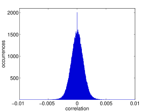
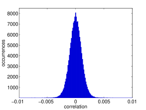
However, Monte-Carlo simulations show that non-diagonal parts of $\langle\eta_{lm}\eta^{*}_{l^{\prime}m^{\prime}}\rangle$ tend to be less than $1\%$ of the diagonal parts. To be specific, we have simulated $5\times 10^{5}$ noise maps for the V and W band respectively by the WMAP noise model (c.f. Eq. 26), and applied the foreground mask KQ75 to them. From the cut-sky simulations, we have estimated the noise covariance matrix $\langle\eta_{lm}\eta^{*}_{l^{\prime}m^{\prime}}\rangle$. The magnitude of noise correlation turns out to decrease with the relative distance in spherical harmonic numbers (i.e. $|l-l^{\prime}|$ and $|m-m^{\prime}|$). In Fig. 1, we show the histogram of noise correlation for the fixed multipole $l=l^{\prime}=400$ and $m\neq m^{\prime}$. Note that the values of the $y$ axis denote the number of $m$ and $m^{\prime}$ pairs, whose correlations correspond to the values of the $x$ axis. As shown in Fig. 1, we find that non-diagonal parts of $\langle\eta_{lm}\eta^{*}_{l^{\prime}m^{\prime}}\rangle$ tend to be less than $1\%$ of the diagonal parts. Besides, we shall be estimating the bispectrum in the multipole range $l\leq 400$, where the Signal-to-Noise Ratio is high (e.g. $17\lesssim C_{l}/N_{l}\lesssim 42$ at $l\leq 400$) [49]. Therefore, we find Eq. 25 provides good approximation for the variance.

Point sources, whose fluxes are below a certain detection threshold, are not properly masked out, and therefore require an accurate assessment of their contribution to the bispectrum. Assuming a Poisson distribution for the point sources [50], their contribution is given by [9, 22, 11]:

$$b_{\mathrm{src}}\,I_{l_{1}l_{2}l_{3}},$$ (28)

where $b_{\mathrm{src}}$ is an amplitude to be determined, and $I_{l_{1}l_{2}l_{3}}$ is given by Eq. 16.

4 Likelihood function

As shown in Eq. 11, CMB bispectrum observables $B^{\mathrm{obs}}_{l_{1}l_{2}l_{3}}$ contain a sum of a large number of terms. In the weak non-Gaussian limit, the correlation between the terms is insignificant:

$$\frac{\langle\left(\begin{array}[]{ccc}l_{1}&l_{2}&l_{3}\\ m_{1}&m_{2}&m_{3}\end{array}\right)\left(\begin{array}[]{ccc}l_{1}&l_{2}&l_{3}\\ m^{\prime}_{1}&m^{\prime}_{2}&m^{\prime}_{3}\end{array}\right)a_{l_{1}m_{1}}a_{l_{2}m_{2}}a_{l_{3}m_{3}}\,(a_{l_{1}m^{\prime}_{1}}a_{l_{2}m^{\prime}_{2}}a_{l_{3}m^{\prime}_{3}})^{*}\rangle}{(C_{l_{1}}+N_{l_{1}})(C_{l_{2}}+N_{l_{2}})(C_{l_{3}}+N_{l_{3}})\Delta_{l_{1}l_{2}l_{3}}}\approx 0,$$ (33)

where we referred to Eq. 25. Accordingly, the distribution of $B^{\mathrm{obs}}_{l_{1}l_{2}l_{3}}$, which contains a large number of weakly correlated random variables, tends toward a Gaussian function by the central limit theorem. It is worth to note that, unlike CMB power spectrum observables, bispectrum observables $B^{\mathrm{obs}}_{l_{1}l_{2}l_{3}}$ contain a sufficiently large number of degree of freedom (e.g. 125) even for the lowest multipole (e.g. $l=2$). Therefore, we may approximate the likelihood function of the CMB bispectrum as follows:

$$\mathcal{L}(B_{l_{1}l_{2}l_{3}}(\lambda_{\alpha})|B^{\mathrm{obs}}_{l_{1}l_{2}l_{3}})=\frac{1}{(2\pi)^{\frac{n}{2}}{\left|\mathbf{C}\right|}^{\frac{1}{2}}}\exp[-\frac{1}{2}(\mathbf{B}^{\mathrm{obs}}-\mathbf{B}(\lambda_{\alpha}))^{\dagger}\,{\mathbf{C}}^{-1}\,(\mathbf{B}^{\mathrm{obs}}-\mathbf{B}(\lambda_{\alpha}))],$$ (34)

where $\mathbf{C}$ is a $n\times n$ covariance matrix, $\lambda_{\alpha}$ are the parameters: $\{f^{\mathrm{local}}_{\mathrm{NL}},f^{\mathrm{equil}}_{\mathrm{NL}},b_{\mathrm{src}}\}$ + cosmological parameters, and $\mathbf{B}^{\mathrm{obs}}$ and $\mathbf{B}(\lambda_{\alpha})$ are vectors consisting of the observed and the theoretical bispectrum respectively. The theoretical bispectrum $\mathbf{B}(\lambda_{\alpha})$ is given by:

$$B_{l_{1}l_{2}l_{3}}(\lambda_{\alpha})=w_{l_{1}}w_{l_{2}}w_{l_{3}}\,f_{\mathrm{sky}}[f^{\mathrm{local}}_{\mathrm{NL}}\,B^{\mathrm{local}}_{l_{1}l_{2}l_{3}}(\lambda_{\alpha})+f^{\mathrm{equil}}_{\mathrm{NL}}\,B^{\mathrm{equil}}_{l_{1}l_{2}l_{3}}+b_{\mathrm{src}}\,I_{l_{1}l_{2}l_{3}}],$$ (35)

where $w_{l}$ is the effective window function, which is the product of the beam transfer function and the pixel window function.

Figure 2: Correlation between CMB power spectrum and bispectrum: $\langle B_{l_{1},l_{2},l_{3}}\>C_{l}\rangle$

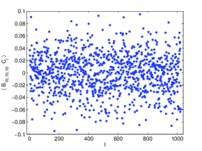
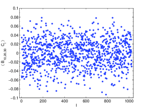
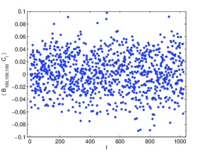
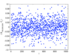
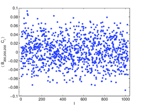
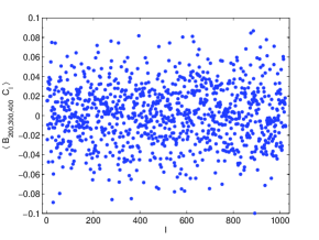
In order to derive a total likelihood, we have investigated the correlation between CMB power spectrum and bispectrum. Due to the complexity of analytic derivation, we have made numerical investigation, using simulations produced by [51]. The simulations are provided in such a way that we may set the value of $f^{\mathrm{local}}_{\mathrm{NL}}$. In Fig. 2, we show the correlation estimated from 1000 simulations, where $f^{\mathrm{local}}_{\mathrm{NL}}$ is set to 40. As shown in Fig. 2, we find the correlation between the CMB power spectrum and bispectrum is insignificant. Therefore, to a good approximation, we may construct a full likelihood function as follows:

$$\mathcal{L}(C_{l}|C^{\mathrm{obs}}_{l})\times\mathcal{L}(B_{l_{1}l_{2}l_{3}}(\lambda_{\alpha})|B^{\mathrm{obs}}_{l_{1}l_{2}l_{3}}),$$ (36)

where $\mathcal{L}(\bar{C}_{l}|C_{l})$ is the likelihood function associated with CMB power spectrum, whose approximate and optimal expression is found in [52]. The corresponding log-likelihood is given by:

$$\log\mathcal{L}(C_{l}|C^{\mathrm{obs}}_{l})+\log\mathcal{L}(B_{l_{1}l_{2}l_{3}}(\lambda_{\alpha})|B^{\mathrm{obs}}_{l_{1}l_{2}l_{3}}).$$ (37)

The log-likelihood of the WMAP CMB power spectrum, which corresponds to the first term in Eq. 37, is provided by the WMAP team’s code and well-integrated into the widely used Monte-Carlo sampling code (i.e. CosmoMC). Therefore, we are going to be mainly concerned with adding the second term of Eq. 37 to the existing code.

As shown in Eq. 37, the likelihood function has dependency on several cosmological parameters. Therefore, we are going to explore multi-dimensional parameter space via MCMC sampling. In this way, we are going to simultaneously fit all cosmological parameters, including $f_{\mathrm{NL}}$.

5 Analysis of the WMAP data

We have co-added WMAP 7 year foreground-reduced maps of the V band and the W band, and applied the KQ75 mask to the co-added map [46, 47, 1]. From the masked V+W map, we have estimated $B^{\mathrm{obs}}_{l_{1}l_{2}l_{3}}$ up to $l\leq 400$ via Eq. 11, where the Wigner 3j symbols have been computed efficiently using the recurrence relation [53]. It took several hours to compute $B^{\mathrm{obs}}_{l_{1}l_{2}l_{3}}$ ($l\leq 400$), which is, however, a manageable one-time cost.

Figure 3: The likelihoods of $f_{\mathrm{NL}}$ and $b_{\mathrm{src}}$: solid (dotted) lines denote the marginalized (mean) likelihood.

Figure 4: Marginalized likelihoods in the plane of $f_{\mathrm{NL}}$ versus cosmological parameters: the contour lines denote 1 and 2 $\sigma$ intervals.

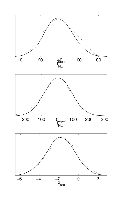
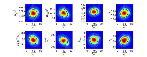
We modified the CosmoMC package so that we can include the bispectrum likelihood (i.e. Eq. 34) and parameters ($\{f^{\mathrm{local}}_{\mathrm{NL}},f^{\mathrm{equil}}_{\mathrm{NL}},b_{\mathrm{src}}\}$) in the Markov Chain Monte Carlo (MCMC) analysis [45, 54]. Note that the power spectrum likelihood is provided by the WMAP team and is already integrated into the CosmoMC package. In order to avoid unnecessary computations, we have added $f_{\mathrm{NL}}$ and $b_{\mathrm{src}}$ as amplitude parameters so that a radiation transfer function (i.e. $g_{l}(k)$ in Eq. 6) or the normalized bispectrum (i.e. Eq. 12 and LABEL:B_equil) is not re-computed for a change of the parameters. For a cosmological model, we have considered $\Lambda$CDM + SZ effect + weak-lensing, where the cosmological parameters are $\lambda\in\{\Omega_{b},\Omega_{c},\tau,n_{s},A_{s},A_{sz},H_{0},f^{\mathrm{local}}_{\mathrm{NL}},f^{\mathrm{equil}}_{\mathrm{NL}},b_{\mathrm{src}}\}$. For data constraints, we have used the WMAP 7 year power spectrum and the bispectrum data described above. By running the modified CosmoMC package [45, 54] on an MPI cluster with 6 chains, we have explored the likelihood in the multi-dimensional parameter space. For a convergence criterion, we have adopted Gelman and Rubin’s “variance of chain means” and set the R-1 statistic to $0.03$ for a stopping criterion [55, 56]. Running a single CPU for each MPI process (total 6 CPUs), we reached the target convergence in less than a day. Once we reached the target convergence, we analyzed the MCMC samples with the CosmoMC package and obtained the parameter likelihood of $f_{\mathrm{NL}}$. In Fig. 3, we show the marginalized and mean likelihoods of $f_{\mathrm{NL}}$ and $b_{\mathrm{src}}$. The marginalized distribution shows the probability in the reduced dimension of parameter space and the mean likelihood is associated with the best-fit value [54]. For a Gaussian distribution, marginalized and mean likelihoods are identical. A shown in Fig. 3, there exist slight discrepancies between the marginalized and mean likelihoods, which indicate the deviation of the parameter likelihood from a Gaussian shape.

Figure 5: MCMC samples: the $x$ and $y$ coordinates correspond to the values of $f^{\mathrm{local}}_{\mathrm{NL}}$ and $f^{\mathrm{equil}}_{\mathrm{NL}}$, color-coded according to the value of $b_{\mathrm{src}}$, marginalized over cosmological parameters.

Table 1: The best-fit values and 68% confindence intervals for $f_{\mathrm{NL}}$ and the cosmological parameters: ($\Lambda$CDM + sz + lens)

parameter	estimate
$f^{\mathrm{local}}_{\mathrm{NL}}$	$39^{+13}_{-14}$
$f^{\mathrm{equil}}_{\mathrm{NL}}$	$-76<f^{\mathrm{equil}}_{\mathrm{NL}}<88$
$b_{\mathrm{src}}$ [$10^{-5}\mu\mathrm{K}^{3}\,\mathrm{sr}^{2}]$	$-2.4^{+2}_{-0.9}$
$\Omega_{b}\,h^{2}$	$0.0225^{+0.0007}_{-0.0005}$
$\Omega_{c}\,h^{2}$	$0.113^{+0.003}_{-0.008}$
$\tau$	$0.083^{+0.013}_{-0.002}$
$n_{s}$	$0.967^{+0.017}_{-0.011}$
$\log[10^{10}A_{s}]$	$3.183^{+0.037}_{-0.06}$
$A_{\mathrm{sz}}$	$1.42^{+0.58}_{-1.42}$
$H_{0}$ [km/s/Mpc]	$70.35^{+3.19}_{-1.8}$

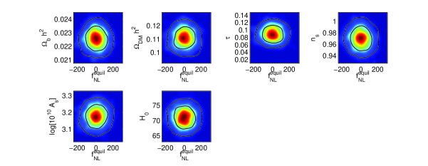
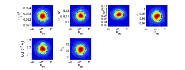
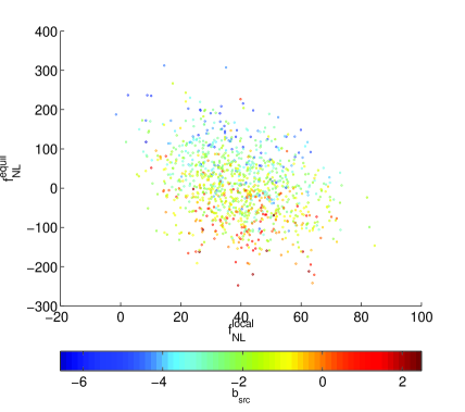
In Fig. 4, we have plotted the marginalized likelihoods in the plane of $f_{\mathrm{NL}}$ versus other parameters. As shown in Fig. 4, there exist non-negligible deviations of the parameter likelihoods from a Gaussian shape. To be specific, the shape of parameter likelihood (e.g. contours of the same color) are poorly fitted by a Gaussian function. In Fig. 5, we show the MCMC samples, where the $x$ and $y$ coordinates correspond to the values of $f^{\mathrm{local}}_{\mathrm{NL}}$ and $f^{\mathrm{equil}}_{\mathrm{NL}}$, and the value of $b_{\mathrm{src}}$ is color-coded. Note that MCMC samples shown in Fig. 5 are obtained after marginalized over the cosmological parameters. In Table 1, we show the best-fit values and 1$\sigma$ intervals for the cosmological parameters as well as for $f_{\mathrm{NL}}$. As shown in Fig. 3 and Table 1, our result is in good agreement with the current results on $f_{\mathrm{NL}}$ and the WMAP concordance model [22, 28]. However, the confidence interval on $f^{\mathrm{local}}_{\mathrm{NL}}$ is different, which we attribute to a difference in the confidence interval estimation. While we have estimated the confidence interval by making a full exploration of the parameter likelihood, most of the existing works have relied on a Fisher matrix, which yields accurate results only for a parameter likelihood of a Gaussian shape.

6 Discussion

We have made an integrated MCMC analysis of the primordial non-Gaussianity ($f_{\mathrm{NL}}$), using the WMAP bispectrum and power spectrum. In our analysis, we have simultaneously constrained $f_{\mathrm{NL}}$ and the cosmological parameters so that the uncertainties of the cosmological parameters can properly propagate into the $f_{\mathrm{NL}}$ estimation. From the parameter likelihoods deduced from the MCMC samples, we find that the parameter likelihood slightly deviates from a Gaussian shape, which makes the Fisher matrix estimation less accurate. Therefore, we have estimated the confidence intervals by exploring the parameter likelihood without using a Fisher matrix. We find that our best-fit values agree well with the existing results. However, we find that the confidence interval is slight different, which we attribute to the difference in the confidence estimation. Mostly due to the increase in the number of parameters, our approach requires a much higher computational load than the estimator of fixed cosmological parameters. However, with further optimization, our approach will be also feasible for the high angular resolution Planck data.

7 Acknowledgments

We are grateful to the anonymous referee for thorough reading and comments, which greatly helped us to improve the clarity of this paper. We thank Pavel Naselsky, Hael Collins, Eiichiro Komatsu and Anthony Lewis for helpful discussions. We acknowledge the use of the Legacy Archive for Microwave Background Data Analysis (LAMBDA), and the non-Gaussianity simulations produced by [51]. This work made use of HEALPix [57, 58] and the CosmoMC package. This work is supported in part by Danmarks Grundforskningsfond, which allowed the establishment of the Danish Discovery Center. This work was supported by FNU grant 272-06-0417, 272-07-0528 and 21-04-0355.

References

- [1] N. Jarosik, C. L. Bennett, J. Dunkley, B. Gold, M. R. Greason, M. Halpern, R. S. Hill, G. Hinshaw, A. Kogut, E. Komatsu, D. Larson, M. Limon, S. S. Meyer, M. R. Nolta, N. Odegard, L. Page, K. M. Smith, D. N. Spergel, G. S. Tucker, J. L. Weiland, E. Wollack, and E. L. Wright. Seven-Year Wilkinson Microwave Anisotropy Probe (WMAP) Observations: Sky Maps, Systematic Errors, and Basic Results. 2010. arXiv:1001.4744.
- [2] C. L. Reichardt and et al. High-Resolution CMB Power Spectrum from the Complete ACBAR Data Set. Astrophys. J., 694:1200–1219, April 2009. arXiv:0801.1491.
- [3] C. Pryke and et al. Second and third season QUaD CMB temperature and polarization power spectra. Astrophys. J., 692:1247, 2009. arXiv:0805.1944.
- [4] The Planck Collaboration. The Scientific Programme of Planck. April 2006. arXiv:astro-ph/0604069.
- [5] J. A. Tauber, N. Mandolesi, J.-L. Puget, T. Banos, M. Bersanelli, F. R. Bouchet, R. C. Butler, J. Charra, G. Crone, J. Dodsworth, and et al. Planck pre-launch status: The Planck mission. Astron. Astrophys., 520:A1+, September 2010.
- [6] Scott Dodelson. Modern Cosmology. Academic Press, 2nd edition, 2003.
- [7] Andrew R. Liddle and David H. Lyth. Cosmological Inflation and Large-Scale Structure. Cambridge University Press, 1st edition, 2000.
- [8] Viatcheslav Mukhanov. Physical Foundations of Cosmology. Cambridge University Press, 1st edition, 2005.
- [9] E. Komatsu. The Pursuit of Non-Gaussian Fluctuations in the Cosmic Microwave Background. PhD thesis, Tohoku University, 2001.
- [10] N. Bartolo, E. Komatsu, S. Matarrese, and A. Riotto. Non-Gaussianity from inflation: theory and observations. Physics Reports, 402:103–266, November 2004.
- [11] E. Komatsu. Hunting for primordial non-Gaussianity in the cosmic microwave background. Classical and Quantum Gravity, 27(12):124010–+, June 2010. arXiv:1003.6097.
- [12] J. Kim and P. Naselsky. Primordial non-Gaussianity and perturbations beyond the present horizon. Phys. Rev. D, 79(12):123006–+, June 2009. arXiv:0905.1781.
- [13] J.C. Mather, D.J. Fixsen, R.A. Shafer, Mosier C., and D.T. Wilkinson. Calibrator design for the cobe far infrared absolute spectrophotometer. Astrophys. J., 512:511, 1999.
- [14] D. J. Fixsen, E. S. Cheng, J. M. Gales, J. C. Mather, R. A. Shafer, and E. L. Wright. The cosmic microwave background spectrum from the full COBE FIRAS data set. Astrophys. J., 473:576, 1996.
- [15] C. L. Bennett, A. J. Banday, K. M. Gorski, G. Hinshaw, P. Jackson, P. Keegstra, A. Kogut, G. F. Smoot, D. T. Wilkinson, and E. L. Wright. Four-year cobe dmr cosmic microwave background observations: Maps and basic results. Astrophys. J. Lett., 464:1, 1996.
- [16] E. Komatsu, A. Kogut, M. R. Nolta, C. L. Bennett, M. Halpern, G. Hinshaw, N. Jarosik, M. Limon, S. S. Meyer, L. Page, D. N. Spergel, G. S. Tucker, L. Verde, E. Wollack, and E. L. Wright. First-Year Wilkinson Microwave Anisotropy Probe (WMAP) Observations: Tests of Gaussianity. Astrophys. J., 148:119–134, September 2003.
- [17] G. Hinshaw and et al. Three-year Wilkinson Microwave Anisotropy Probe (WMAP) observations: Temperature analysis. Astrophys. J., 170:288, 2007.
- [18] E. Komatsu, B. D. Wandelt, D. N. Spergel, A. J. Banday, and K. M. Górski. Measurement of the Cosmic Microwave Background Bispectrum on the COBE DMR Sky Maps. Astrophys. J., 566:19–29, February 2002. arXiv:astro-ph/0107605.
- [19] A. P. S. Yadav and B. D. Wandelt. Evidence of Primordial Non-Gaussianity () in the Wilkinson Microwave Anisotropy Probe 3-Year Data at 2.8. Physical Review Letters, 100(18):181301–+, May 2008. arXiv:0712.1148.
- [20] P. Creminelli, L. Senatore, M. Zaldarriaga, and M. Tegmark. Limits on f_NL parameters from Wilkinson Microwave Anisotropy Probe three-year data. JCAP, 3:5–+, March 2007. arXiv:astro-ph/0610600.
- [21] P. Cabella, F. K. Hansen, M. Liguori, D. Marinucci, S. Matarrese, L. Moscardini, and N. Vittorio. The integrated bispectrum as a test of cosmic microwave background non-Gaussianity: detection power and limits on f_NL with WMAP data. Mon. Not. R. Astron. Soc., 369:819–824, June 2006. arXiv:astro-ph/0512112.
- [22] E. Komatsu and et al. Five-Year Wilkinson Microwave Anisotropy Probe Observations: Cosmological Interpretation. Astrophys. J., 180:330–376, February 2009. arXiv:0803.0547.
- [23] K. M. Smith, L. Senatore, and M. Zaldarriaga. Optimal limits on from WMAP 5-year data. ArXiv e-prints, January 2009. arXiv:0901.2572.
- [24] A. Curto, J. F. Macías-Pérez, E. Martínez-González, R. B. Barreiro, D. Santos, F. K. Hansen, M. Liguori, and S. Matarrese. Constraints on the non-linear coupling parameter f_nl with Archeops data. Astron. Astrophys., 486:383–391, August 2008. arXiv:0804.0136.
- [25] P. Natoli, G. de Troia, C. Hikage, E. Komatsu, M. Migliaccio, P. A. R. Ade, J. J. Bock, J. R. Bond, J. Borrill, A. Boscaleri, C. R. Contaldi, B. P. Crill, P. de Bernardis, G. de Gasperis, A. de Oliveira-Costa, G. di Stefano, E. Hivon, T. S. Kisner, W. C. Jones, A. E. Lange, S. Masi, P. D. Mauskopf, C. J. MacTavish, A. Melchiorri, T. E. Montroy, C. B. Netterfield, E. Pascale, F. Piacentini, G. Polenta, S. Ricciardi, G. Romeo, J. E. Ruhl, M. Tegmark, M. Veneziani, and N. Vittorio. BOOMERanG constraints on primordial non-Gaussianity from analytical Minkowski functionals. Mon. Not. R. Astron. Soc., 408:1658–1665, November 2010. arXiv:0905.4301.
- [26] Ø. Rudjord, F. K. Hansen, X. Lan, M. Liguori, D. Marinucci, and S. Matarrese. An Estimate of the Primordial Non-Gaussianity Parameter fNL Using the Needlet Bispectrum from WMAP. Astrophys. J., 701:369–376, August 2009.
- [27] A. Curto, E. Martínez-González, P. Mukherjee, R. B. Barreiro, F. K. Hansen, M. Liguori, and S. Matarrese. Wilkinson Microwave Anisotropy Probe 5-yr constraints on fnl with wavelets. Mon. Not. R. Astron. Soc., 393:615–622, February 2009. arXiv:0807.0231.
- [28] E. Komatsu and et al. Seven-Year Wilkinson Microwave Anisotropy Probe (WMAP) Observations: Cosmological Interpretation. January 2010. arXiv:1001.4538.
- [29] B. Casaponsa, R. B. Barreiro, A. Curto, E. Martínez-González, and P. Vielva. Wilkinson Microwave Anisotropy Probe 7-yr constraints on fNL with a fast wavelet estimator. ArXiv e-prints, September 2010. arXiv:1009.0632.
- [30] T. Falk, R. Rangarajan, and M. Srednicki. The angular dependence of the three-point correlation function of the cosmic microwave background radiation as predicted by inflationary cosmologies. Astrophys. J. Lett., 403:L1–L3, January 1993.
- [31] M. Liguori, S. Matarrese, and L. Moscardini. High-Resolution Simulations of Non-Gaussian Cosmic Microwave Background Maps in Spherical Coordinates. Astrophys. J., 597:57–65, November 2003.
- [32] P. McDonald. Primordial non-Gaussianity: Large-scale structure signature in the perturbative bias model. Phys. Rev. D, 78(12):123519–+, 2008. arXiv:0806.1061.
- [33] J. Maldacena. Non-gaussian features of primordial fluctuations in single field inflationary models. Journal of High Energy Physics, 5:13–+, May 2003.
- [34] L. Senatore, K. M. Smith, and M. Zaldarriaga. Non-Gaussianities in single field inflation and their optimal limits from the WMAP 5-year data. JCAP, 1:28–+, January 2010. arXiv:0905.3746.
- [35] A. P. S. Yadav and B. D. Wandelt. Primordial Non-Gaussianity in the Cosmic Microwave Background. June 2010. arXiv:1006.0275.
- [36] P. Creminelli and M. Zaldarriaga. A single-field consistency relation for the three-point function. JCAP, 10:6–+, October 2004. arXiv:astro-ph/0407059.
- [37] X. Chen, M.-x. Huang, S. Kachru, and G. Shiu. Observational signatures and non-Gaussianities of general single-field inflation. JCAP, 1:2–+, January 2007. arXiv:hep-th/0605045.
- [38] D. Seery and J. E. Lidsey. Primordial non-Gaussianities in single-field inflation. JCAP, 6:3–+, June 2005. arXiv:astro-ph/0503692.
- [39] C. Cheung, A. L. Fitzpatrick, J. Kaplan, L. Senatore, and P. Creminelli. The effective field theory of inflation. JCAP, 3:14–014, March 2008. arXiv:0709.0293.
- [40] R. Holman and A. J. Tolley. Enhanced non-Gaussianity from excited initial states. JCAP, 5:1–+, May 2008. arXiv:0710.1302.
- [41] I. G. Moss and C. Xiong. Non-Gaussianity in fluctuations from warm inflation. JCAP, 4:7–+, April 2007.
- [42] X. Chen and Y. Wang. Quasi-single field inflation and non-Gaussianities. JCAP, 4:27–+, April 2010. arXiv:0911.3380.
- [43] I. G. Moss and C. M. Graham. Testing models of inflation with cosmic microwave background non-Gaussianity. JCAP, 11:4–+, November 2007. arXiv:0707.1647.
- [44] W. Hu and M. White. CMB anisotropies: Total angular momentum method. Phys. Rev. D, 56:596–+, July 1997.
- [45] Antony Lewis, Anthony Challinor, and Anthony Lasenby. Efficient computation of CMB anisotropies in closed FRW models. Astrophys. J., 538:473, 2000. http://camb.info/.
- [46] B. Gold and et al. Five-Year Wilkinson Microwave Anisotropy Probe Observations: Galactic Foreground Emission. Astrophys. J., 180:265–282, February 2009. arXiv:0803.0715.
- [47] B. Gold, N. Odegard, J. L. Weiland, R. S. Hill, A. Kogut, C. L. Bennett, G. Hinshaw, J. Dunkley, M. Halpern, N. Jarosik, E. Komatsu, D. Larson, M. Limon, S. S. Meyer, M. R. Nolta, L. Page, K. M. Smith, D. N. Spergel, G. S. Tucker, E. Wollack, and E. L. Wright. Seven-Year Wilkinson Microwave Anisotropy Probe (WMAP) Observations: Galactic Foreground Emission. January 2010. arXiv:1001.4555.
- [48] P. Creminelli, A. Nicolis, L. Senatore, M. Tegmark, and M. Zaldarriaga. Limits on non-Gaussianities from WMAP data. JCAP, 5:4–+, May 2006.
- [49] D. Larson, J. Dunkley, G. Hinshaw, E. Komatsu, M. R. Nolta, C. L. Bennett, B. Gold, M. Halpern, R. S. Hill, N. Jarosik, A. Kogut, M. Limon, S. S. Meyer, N. Odegard, L. Page, K. M. Smith, D. N. Spergel, G. S. Tucker, J. L. Weiland, E. Wollack, and E. L. Wright. Seven-Year Wilkinson Microwave Anisotropy Probe (WMAP) Observations: Power Spectra and WMAP-Derived Parameters. 2010. arXiv:1001.4635.
- [50] L. Toffolatti, F. Argueso Gomez, G. de Zotti, P. Mazzei, A. Franceschini, L. Danese, and C. Burigana. Extragalactic source counts and contributions to the anisotropies of the cosmic microwave background: predictions for the Planck Surveyor mission. Mon. Not. R. Astron. Soc., 297:117–127, 1998.
- [51] F. Elsner and B. D. Wandelt. Improved Simulation of Non-Gaussian Temperature and Polarization Cosmic Microwave Background Maps. Astrophys.J.Suppl., 184:264–270, October 2009. arXiv:0909.0009.
- [52] L. Verde, H. V. Peiris, D. N. Spergel, M. Noltaand C. L. Bennettand M. Halpernand G. Hinshawand N. Jarosikand A. Kogutand M. Limon, and S. S. Meyerand L. Pageand G. S. Tuckerand E. Wollackand E. L. Wright. First year wilkinson microwave anisotropy probe (WMAP) observations: Parameter estimation methodology. Astrophys. J., 148:195, 2003.
- [53] Klaus Schulten and Roy G. Gordon. Exact recursive evaluation of 3-j and 6-j coefficients for quantum-mechanical coupling of angular momenta. J. Math. Phys, 16:1961, 1975.
- [54] Antony Lewis and Sarah Bridle. Cosmological parameters from CMB and other data: a Monte-Carlo approach. Phys. Rev. D, 66:103511, 2002.
- [55] Andrew Gelman and Donald B. Rubin. Inference from iterative simulation using multiple sequences. Statistical Science, 7:457, 1992.
- [56] Stephen Brooks and Andrew Gelman. General methods for monitoring convergence of iterative simulations. Journal of Computational and Graphical Statistics, 7(4):434, 1998.
- [57] K. M. Gorski, B. D. Wandelt, F. K. Hansen, E. Hivon, and A. J. Banday. The HEALPix Primer. May 1999. arXiv:astro-ph/9905275.
- [58] K. M. Gorski, E. Hivon, A. J. Banday, B. D. Wandelt, F. K. Hansen, M. Reinecke, and M. Bartelman. HEALPix – a framework for high resolution discretization, and fast analysis of data distributed on the sphere. Astrophys. J., 622:759, 2005.