Longitudinal and Transverse Breathing Oscillations
in Bose - Fermi Mixtures of Yb atoms at Zero Temperature
in the Largely Prolate Deformed Traps

Abstract

We study the breathing oscillations in bose-fermi mixtures of Yb isotopes in the largely prolate deformed trap, which are realized by Kyoto group. We take three combinations of the Yb isotopes, ¹⁷⁰Yb-¹⁷¹Yb , ¹⁷⁰Yb-¹⁷³Yb and ¹⁷⁴Yb-¹⁷³Yb , whose boson-fermion interactions are weakly repulsive, strongly attractive and strongly repulsive. The collective oscillations in the deformed trap are calculated in the dynamical time-development approach, which is formulated with the time-dependent Gross-Pitaevskii and the Vlasov equations. We analyze the results with the intrinsic oscillation modes of the deformed system, obtained in the scaling method, and show that the damping and forced-oscillation effects of the intrinsic modes explain time-variation behaviors of oscillations, especially, in the fermion transverse mode.

I Introduction

In this decade, there have been significant progresses in the production of ultracold gases, which realize the Bose-Einstein condensates (BEC) nobel ; Dalfovo ; becth ; Andersen , two boson mixtures Truscott ; B-B , degenerate atomic Fermi gases ferG , and Bose-Fermi (BF) mixing gases Truscott ; Schreck ; BferM ; Modugno . In particular the BF mixtures attract physical interest as a typical example in which particles obeying different quantum statistics are intermingled. Using the system we have a very big opportunity to obtain various new knowledge of many-body quantum systems because we can make a large variety of combinations of atomic species and control the atomic interactions using the Feshbach resonance Fesh .

Theoretical studies of the BF mixtures have been done on static properties Molmer ; Amoruso ; MOSY ; Bijlsma ; Vichi ; Vichi1 , the phase diagram and phase separation Nygaard ; Yi ; Viverit ; Capuzzi02 , stability MSY1 ; Roth ; Capuzzi03 and collective excitations MSY ; Minguzzi ; MOSY ; zeros ; Yip ; sogo ; tomoBF ; monoEX ; tbDPL ; QPBF .

Recently Kyoto university group has performed researches on the trapped atomic gases of the Yb isotopes: the BEC Takasu and the Fermi-degeneracy Fukuhara1 . They also succeeded in realizing the BF mixtures of the isotopes. The Yb consists of many kinds of isotopes— five bosons (^{168,170,172,174,176}Yb) and two fermions (^171,173Yb), which give a variety of combinations in the BF mixtures. The scattering lengths of the boson-fermion interactions have been determined experimentally by the group Fukuhara1 ; Fukuhara2 ; Kitagawa ; Fukuhara3 ; Fukuhara-M , and the experimental studies of the ground state properties and the collective oscillations of the BF mixtures is now under progressing.

In many characteristic properties, the spectrum of the collective excitations is an important diagnostic signal of these systems; they commonly appear in many-particle systems and are often sensitive to the inter-particle interaction and the structure of the ground and excited states.

We have constructed a dynamical approach to solve time-developments of the oscillation states with the time-dependent Gross-Pitaevskii (TDGP) and Vlasov equations, and have studied the monopole tomoBF ; monoEX and dipole oscillations tbDPL of the BF mixtures. In these works, we have found that the oscillational motions of the BF mixtures include various modes such as the boson and fermion intrinsic and the forced oscillation modes, and that the intrinsic frequencies of these modes obtained in the dynamical calculation are different from those in the sum-rule MOSY ; MSY and the scaling scal ; scalDP ; scalTF ; scalTF2 approaches, which are approximations of the random phase approximation (RPA) zeros ; sogo . Furthermore, the dynamical calculations are consistent with the results in RPA only in early stage of time, but show discrepancies in later stage of time, and, as the boson-fermion interaction becomes stronger, the discrepancies come to appear earlier in oscillation. Thus the BF mixtures show new dynamical properties different from the other finite many-body systems such as atomic nuclei.

In this paper, we take three combinations of the Yb isotopes, ¹⁷⁰Yb-¹⁷¹Yb , ¹⁷⁰Yb-¹⁷³Yb and ¹⁷⁴Yb-¹⁷³Yb , where the boson-fermion interactions are weakly repulsive, strongly attractive and strongly repulsive. In the previous paper QPBF , we have calculated the quadrupole oscillation of these mixtures in the spherical trap, and compared the results with those obtained in RPA. The RPA gives small-amplitude intrinsic modes of the mixtures and describes the whole oscillations as linear combinations of these intrinsic modes. When the boson-fermion interaction is weak and/or the amplitude is small, the linearly-combined oscillations can be good approximation, and the RPA gives the results consistent with those in the dynamical approach. However, when the boson-fermion interaction is strong or the amplitude is large, the oscillations of the BF mixtures obtained in the dynamical approach show very different behaviors from those obtained in the RPA. For example, in the strongly-attractive boson-fermion interaction, the fermi gas overflows from the boson occupation region and makes large expansion, which leads to a monopole oscillation mode, and, in the case of the strongly-repulsive interaction, the fermion intrinsic-mode shows rapid damping so that the fermi gas comes to co-oscillate with the bose gas QPBF .

In actual experiments, the largely-deformed trap of axial-symmetry is used, and the oscillation behaviors should be different from those in the spherical trap. The monopole and quadrupole oscillations, which are coupled in axial-symmetric traps, are recombined into two modes oscillating along the symmetric axial and the transverse directions. Such behaviors are observed in the two-component fermi-gas oscillations scalTF2 , but no studies have been done for the BF mixture.

In this paper, we investigate the breathing oscillations of the BF mixtures in the largely deformed system of the prolate shape. Then we examine oscillation behaviors along the longitudinal and transverse directions separately, which are the symmetry axis and the directions perpendicular to it, respectively.

In the next section, we explain a microscopic model of the BF mixtures, and examine the intrinsic collective modes and their coupling behaviors in the scaling method. In Sec. III, we show the time-development calculations in the TDHF+Vlasov approach for the breathing oscillations in the BF mixture, and discuss their properties on the basis of the collective modes obtained in the scaling method. The summary of the present work is given in Sec. IV.

II Collective Oscillations in Scaling Method

Before presenting actual time-development calculations we consider the oscillation behaviors in the deformed system, and take up the collective modes from the macroscopic point of view.

The deformed BF mixtures have the breathing oscillations, which are generally coupled modes of the monopole and quadrupole oscillations. The mode-structure of breathing oscillations in the deformed system has been studied, for example, in two-component fermi gas scalTF2 , but it is not clear for the deformed BF mixtures. Thus, in the present section, we should clarify the mode-structure of the breathing oscillations in the deformed BF mixture using the scaling method as in Ref. sumF ; it is a macroscopic approximation consistent with the energy-weighted sum rules bohi .

The scaling method describe the collective oscillations within the linear response regime. However, the method has been extended in the nonlinear case with contributions of the nonlinear terms. The nonlinear calculations was applied to the oscillations of BEC CD96 , which reproduced the experimental results by Ref. Mewes96 very well. Also, the method was used in the study of the BEC with non-condensed bosons KSS96 .

II.1 Total Energy of BF mixtures and Scaled Variables

In this work we consider the mixture of dilute boson and one-component-fermion gases at zero temperature in an axially symmetric trapping potential, the symmetry axis of which is chosen to be the $z$-axis. We assume zero-range interactions between atoms, and no fermion-fermion interactions. Using the Hartree-Fock approximation, the total energy is given by a functional of the condensed boson wave function $\phi_{c}$, and the $n$-th fermion single-particle wave functions $\psi_{n}$:

$$E_{T} = \int d^{3}{r}\Bigg{[}-\frac{1}{2}\nabla_{r}\phi_{c}^{\dagger}(\mbox{$\bm{r}$})\nabla_{r}\phi_{c}(\mbox{$\bm{r}$})+\frac{1}{2}(\mbox{$\bm{r}$}_{T}^{2}+\kappa_{L}^{2}z^{2})\phi_{c}^{\dagger}(\mbox{$\bm{r}$})\phi_{c}(\mbox{$\bm{r}$})+\frac{g_{BB}}{2}\{\phi_{c}^{\dagger}(\mbox{$\bm{r}$})\phi_{c}(\mbox{$\bm{r}$})\}^{2}$$ (1)

$$\qquad\quad+\frac{1}{2m_{f}}\sum_{n}\nabla_{r}\psi_{n}^{\dagger}(\mbox{$\bm{r}$})\nabla_{r}\psi_{n}(\mbox{$\bm{r}$})+\frac{1}{2}m_{f}\omega_{f}^{2}(\mbox{$\bm{r}$}_{T}^{2}+\kappa_{L}^{2}z^{2})\sum_{n}\psi_{n}^{\dagger}(\mbox{$\bm{r}$})\psi_{n}(\mbox{$\bm{r}$})$$

$$\qquad\quad+h_{BF}\phi_{c}^{\dagger}(\mbox{$\bm{r}$})\phi_{c}(\mbox{$\bm{r}$})\sum_{n}\psi_{n}^{\dagger}(\mbox{$\bm{r}$})\psi_{n}(\mbox{$\bm{r}$})\Bigg{]}.$$

In the above equation all the variables are dimensionless. The spatial coordinate $\bm{r}$ is scaled with $(\hbar/M_{B}\Omega_{B})^{1/2}$, where $M_{B}$ and $\Omega_{B}$ are the boson mass and boson transverse trapped frequency, $m_{f}$ and $\omega_{f}$ are the fermion-to-boson ratios of the mass and the trapping-potential frequency, and $g_{BB}$ and $h_{BF}$ are the dimensionless coupling constants of the boson-boson and boson-fermion interactions; the detailed definitions are given in Ref.  tomoBF ; tbDPL ; QPBF .

Here the scaled wave functions are introduced from the ground-state one-body wave functions, $\phi_{c}^{(g)}$ and $\psi^{(g)}_{n}$:

$$\phi_{\lambda}(\mbox{$\bm{r}$},\tau) = e^{i\xi_{B}(\mbox{$\bm{r}$},\tau)}e^{\lambda_{BT}(\tau)+\frac{1}{2}\lambda_{BL}(\tau)}\phi_{c}^{(g)}(e^{\lambda_{BT}(\tau)}\mbox{$\bm{r}$}_{T};e^{\lambda_{BL}(\tau)}z),$$ (2)

$$\psi_{\lambda,n}(\mbox{$\bm{r}$},\tau) = e^{im_{f}\xi_{F}(\mbox{$\bm{r}$},\tau)}e^{\lambda_{FT}(\tau)+\frac{1}{2}\lambda_{FL}(\tau)}\psi_{n}^{(g)}(e^{\lambda_{FT}(\tau)}\mbox{$\bm{r}$}_{T};e^{\lambda_{FL}(\tau)}z)$$ (3)

where $\tau$ is the dimensionless time coordinate scaled with $\Omega_{B}$, and $B$ and $F$ denote the boson and fermion, respectively. The factor $\exp(i\xi_{a})$ is the Gallilei-transformation factor, which is necessary for the scaled wave functions to satisfy the continuum equation, and the phase parameters $\xi_{a}(\mbox{$\bm{r}$},\tau)$ are given by

$$\xi_{a}(\mbox{$\bm{r}$},\tau)=\frac{1}{2}\left[{\dot{\lambda}}_{Ta}(\tau)\mbox{$\bm{r}$}_{T}^{2}+{\dot{\lambda}}_{La}(\tau)z^{2}\right],\qquad(a=B,F)$$ (4)

The variables, $\lambda_{BT}$, $\lambda_{BL}$, $\lambda_{FT}$, $\lambda_{FL}$, are the collective coordinates describing the boson longitudinal breathing (BLB), boson transverse breathing (BTB), fermion longitudinal breathing (FLB) and fermion transverse breathing (FTB) oscillation modes, and ${\dot{\lambda}}$’s are the time-derivatives of them. As it turns out, the four breathing modes are completely decoupled in the BF mixtures of no interactions: $g_{BB}=h_{BF}=0$.

Here we give a comment on the method of introducing the collective coordinates. In Ref.  CD96 , they introduced the scaling parameters as $r_{i}\rightarrow\lambda^{\prime}_{i}r_{i}$. For the ground state, $\lambda_{i}=0$ in the present paper corresponds to $\lambda^{\prime}_{i}=1$, and, in addition, $\lambda_{i}=-\infty$ corresponds to $\lambda^{\prime}_{i}=0$. For the small amplitude oscillations ($|\lambda_{i}|\ll 1$), the power expansion of the energy of he system with $\lambda_{i}$ should make clear the formal differences of both methods in appearance, while the calculated collective frequencies does not depend on the choice of the method in principle.

Furthermore, one can make a scaled wave function exact by introducing a time-dependent trap frequency and couplings with suitable parameters GBD10 . This method has been used for the analysis of the adiabatic expansions of BEC Campo11 .

Substituting the wave-functions (2,3) into the total energy functional (1), we obtain the total energy:

$$E_{T} = \frac{1}{2}\int d^{3}r\left\{(\nabla_{r}\xi_{B})^{2}\rho_{B}+e^{2\lambda_{BT}}(T_{B,1}+T_{B,2})+e^{2\lambda_{BL}}T_{B,3}\right\}$$ (5)

$$+\frac{1}{2}\int d^{3}r\left\{e^{-2\lambda_{BT}}(r_{1}^{2}+r_{2}^{2})+e^{-2\lambda_{BL}}\kappa_{L}^{2}z^{2})\right\}\rho_{B}(\mbox{$\bm{r}$})$$

$$+\frac{g_{BB}}{2}e^{2\lambda_{BT}+\lambda_{BL}}\int d^{3}r\rho_{B}^{2}(\mbox{$\bm{r}$}),$$

$$+\frac{1}{2m_{f}}\int d^{3}r\left\{m_{f}^{2}(\nabla_{r}\xi_{F})^{2}\rho_{F}+e^{2\lambda_{FT}}(T_{F,1}+T_{F,2})+e^{2\lambda_{FL}}T_{F,3}\right\}$$

$$+\frac{1}{2}m_{f}\omega_{f}^{2}\int d^{3}r\left\{e^{-2\lambda_{FT}}(r_{1}^{2}+r_{2}^{2})+e^{-2\lambda_{FT}}\kappa_{L}^{2}z^{2})\right\}\rho_{F}(\mbox{$\bm{r}$}),$$

$$+h_{BF}e^{2\lambda_{BT}+\lambda_{BL}+2\lambda_{FT}+\lambda_{FL}}\int d^{3}r\,\rho_{B}(e^{\lambda_{BT}}\mbox{$\bm{r}$}_{T};e^{\lambda_{BL}}z)\rho_{F}(e^{\lambda_{FT}}\mbox{$\bm{r}$}_{T};e^{\lambda_{FL}}z),$$

where

$$T_{B,i} = \int d^{3}r\left|\frac{\partial}{\partial r_{i}}\phi(\mbox{$\bm{r}$})\right|^{2},\qquad(i=1,2,3)$$ (6)

$$T_{F,i} = \sum_{n}\int d^{3}{r}\left|\frac{\partial}{\partial r_{i}}\psi_{n}(\mbox{$\bm{r}$})\right|^{2},\qquad(i=1,2,3)$$ (7)

$$\rho_{B}(\mbox{$\bm{r}$}) = N_{b}|\phi_{c}(\mbox{$\bm{r}$})|^{2},\quad\rho_{F}(\mbox{$\bm{r}$})~{}=~{}\sum^{occ}_{n}|\psi_{n}(\mbox{$\bm{r}$})|^{2}.$$ (8)

In order to obtain the ground state of the system we use the Thomas-Fermi (TF) approximation:

$$T_{B}(\mbox{$\bm{r}$})=0,\qquad T_{F,1}(\mbox{$\bm{r}$})=T_{F,2}(\mbox{$\bm{r}$})=T_{F,3}(\mbox{$\bm{r}$})=\frac{1}{5}(6\pi^{2})^{\frac{2}{3}}\left[\rho_{F}(\mbox{$\bm{r}$})\right]^{\frac{5}{3}}.$$ (9)

It should be noted that the momentum distribution is spherically-symmetric. In order to simplify the analytic calculation, we use the dimensionless constants and variables:

$$h =\frac{1}{m_{f}\omega_{f}^{2}}\frac{h_{BF}}{g_{BB}},\quad \bm{x}=\frac{m_{f}^{4}\omega_{f}^{5}g_{BB}}{3\pi^{2}}(r_{1},r_{2},\kappa_{L}z),$$ (10)

$$n_{B} =\frac{2m_{f}^{8}\omega_{f}^{10}g_{BB}^{3}}{9\pi^{4}}\rho_{B},\quad n_{F}=\frac{2m_{f}^{9}\omega_{f}^{12}g_{BB}^{3}}{9\pi^{4}}\rho_{F},$$ (11)

with which the scaled dimensionless total energy is given by:

$$\mbox{${\tilde{E}}_{T}$}^{(0)} = \frac{4\kappa_{L}m_{f}^{28}\omega_{f}^{35}g_{BB}^{8}}{3^{7}\pi^{14}}E_{T}(\mbox{$\bm{\lambda}$}=0,{\dot{}\mbox{$\bm{\lambda}$}}=0)$$ (12)

$$= \int d^{3}{x}\Bigg{\{}x^{2}n_{B}+\frac{1}{2}n_{B}^{2}+\frac{3}{5}n_{F}^{\frac{5}{3}}+x^{2}n_{F}+hn_{B}n_{F}\Bigg{\}},$$

where $x^{2}=|\bm{x}|^{2}$. After the scaling transformation, the ground state depends only on the three variables, $e_{B}$, $e_{F}$ and $h$, and the dependence of the deformation parameter $\kappa_{L}$, the boson-boson coupling $g_{BB}$, the fermion mass $m_{f}$ are eliminated.

From the variations of the total energy with respect to the densities, $\delta{\tilde{E}}^{(0)}/\delta n_{B}=0$ and $\delta{\tilde{E}}^{(0)}/\delta n_{F}=0$ , we obtain the TF equations:

$$n_{B}+hn_{F}=e_{B}-x^{2},\quad n_{F}^{\frac{2}{3}}+hn_{B}=e_{F}-x^{2}.$$ (13)

where $e_{B}$ and $e_{F}$ are the scaled chemical potentials for boson and fermion, respectively, which are written with the chemical potentials for boson $\mu_{B}$ and fermion $\mu_{F}$ as

$$e_{B} = \frac{2m_{f}^{8}\omega_{f}^{10}g_{BB}^{2}}{9\pi^{4}}\mu_{B},$$ (14)

$$e_{F} = \frac{2m_{f}^{7}\omega_{f}^{8}g_{BB}^{2}}{9\pi^{4}}\mu_{F}.$$ (15)

The stability condition of the TF solution is obtained from the second-order variation of the total energy:

$$\frac{\delta^{2}{\tilde{E}}^{(0)}}{\delta n_{B}^{2}}\frac{\delta^{2}{\tilde{E}}^{(0)}}{\delta n_{F}^{2}}-\left(\frac{\delta^{2}{\tilde{E}}^{(0)}}{\delta n_{B}\delta n_{F}}\right)^{2}=\frac{2}{3}n_{F}^{-\frac{1}{3}}-h^{2}>0,$$ (16)

Using (12), it gives the upper limit of the fermion density:

$$n_{F}<\frac{8}{27h^{6}}=\left(\frac{2}{3h^{2}}\right)^{3}.$$ (17)

Furthermore, from Eqs. (13), the spatial derivative of $n_{F}$ is related with $n_{F}$ itself in the TF approximation:

$$\frac{\partial n_{F}}{\partial x^{2}}=\frac{h-1}{\frac{2}{3}n_{F}^{-\frac{1}{3}}-h^{2}}.$$ (18)

Thus it proves that $\partial n_{F}/\partial x^{2}<0$ when $h<1$, and $\partial n_{F}/\partial x^{2}>0$ when $h>1$.

II.2 Collective Oscillations

Now we study the collective oscillation in the scaling method. With the scaling variables, the total energy for collective oscillations (5) is written as

$${\tilde{E}}_{T} = \frac{1}{2}{\tilde{X}}_{B}\left\{\frac{2e^{-2\lambda_{BT}}}{3}{\dot{\lambda}}^{2}_{BT}+\frac{e^{-2\lambda_{BL}}}{3\kappa_{L}^{2}}{\dot{\lambda}}^{2}_{BL}\right\}$$ (19)

$$+\frac{2e^{-2\lambda_{BT}}+e^{-2\lambda_{BL}}}{3}{\tilde{X}}_{B}+e^{2\lambda_{BT}+\lambda_{BL}}V_{bb}$$

$$+\frac{1}{2}{\tilde{X}}_{F}\omega_{f}^{2}\left\{\frac{2e^{-2\lambda_{FT}}}{3}{\dot{\lambda}}^{2}_{FT}+\frac{e^{-2\lambda_{FL}}}{3\kappa_{L}^{2}}{\dot{\lambda}}^{2}_{FL}\right\}$$

$$+\frac{2e^{2\lambda_{FT}}+e^{2\lambda_{FL}}}{3}{\mbox{${\tilde{T}}$}}_{F}+\frac{2e^{-2\lambda_{FT}}+e^{-2\lambda_{FL}}}{3}{\tilde{X}}_{F}+V_{bf}$$

where

$$\mbox{${\tilde{T}}$}_{F} = \frac{3}{5}\int d^{3}{x}\,n_{F}^{\frac{5}{3}}(\bm{x})$$ (20)

$$X_{B,F} = \int d^{3}{x}\,x^{2}n_{B,F}(\bm{x})$$ (21)

$$V_{bb} = \int d^{3}{x}\,n_{B}^{2}(\bm{x})$$ (22)

$$V_{bf} = e^{2\lambda_{BT}+\lambda_{BL}+2\lambda_{FT}+\lambda_{FL}}$$ (23)

$$\times h\int d^{3}{r}\,n_{B}(e^{\lambda_{BT}}\bm{x}_{T},e^{\lambda_{BL}}x_{3})n_{F}(e^{\lambda_{FT}}\bm{x}_{T},e^{\lambda_{FL}}x_{3})$$

Using the vector notation for the collective variables, $\mbox{${}^{t}{\bm{\lambda}}$}=(\lambda_{BT},\lambda_{BL},\lambda_{FT},\lambda_{FL})$, and expanding the total energy to the order of $O(\lambda^{2}$), we obtain the oscillation energy of the system:

$$\Delta{\tilde{E}}_{T}\equiv{\tilde{E}}_{T}-{\tilde{E}}^{(0)}_{T}\approx\frac{1}{2}\mbox{${}^{t}{\bm{\dot{\lambda}}}$}B\mbox{$\bm{\dot{\lambda}}$}+\frac{1}{2}\mbox{${}^{t}{\bm{\lambda}}$}C\mbox{$\bm{\lambda}$}.$$ (24)

The matrices $B$ and $C$ are defined by

$$B=\left(\begin{array}[]{cccc}\frac{4X_{B}}{3}&0&0&0\\ 0&\frac{2}{3\kappa_{L}^{2}}X_{B}&0&0\\ 0&0&\frac{4}{3\omega_{f}^{2}}X_{F}&0\\ 0&0&0&\frac{2}{3\kappa_{L}^{2}\omega_{f}^{2}}X_{F}\\ \end{array}\right),$$ (25)

$$C = \left(\begin{array}[]{cccc}\frac{8}{3}X_{B}+4V_{bb}&2V_{bb}&0&0\\ 2V_{bb}&\frac{4}{3}X_{B}+V_{bb}&0&0\\ 0&0&\frac{8}{3}(\mbox{${\tilde{T}}$}_{F}+X_{F})&0\\ 0&0&0&\frac{4}{3}(\mbox{${\tilde{T}}$}_{F}+X_{F})\\ \end{array}\right)$$ (35)

$$+\left(\begin{array}[]{cccc}~{}-\frac{4}{3}V_{1}-\frac{8}{15}V_{3}{}&~{}-\frac{2}{3}V_{1}-\frac{2}{15}V_{3}{}&~{}\frac{8}{15}V_{3}&\frac{2}{15}V_{3}{}\\ ~{}-\frac{2}{3}V_{1}-\frac{2}{15}V_{3}{}&~{}-\frac{1}{3}V_{1}-\frac{1}{5}V_{3}{}&~{}\frac{2}{15}V_{3}{}&\frac{1}{5}V_{3}{}\\ ~{}\frac{8}{15}V_{3}{}&~{}\frac{2}{15}V_{3}{}&~{}-\frac{4}{3}V_{2}-\frac{8}{15}V_{3}{}&~{}-\frac{2}{3}V_{2}-\frac{2}{15}V_{3}{}\\ ~{}\frac{2}{15}V_{3}&\frac{1}{5}V_{3}{}&~{}-\frac{2}{3}V_{2}-\frac{2}{15}V_{3}{}&-\frac{1}{3}V_{2}-\frac{1}{5}V_{3}\\ \end{array}\right),$$

where

$$V_{1} = h\int d^{3}{x}\,x\,n_{B}\frac{\partial n_{F}}{\partial x},$$ (36)

$$V_{2} = h\int d^{3}{x}\,x\,n_{F}\frac{\partial n_{B}}{\partial x},$$ (37)

$$V_{3} = h\int d^{3}{x}\,x^{2}\frac{\partial n_{B}}{\partial x}\frac{\partial n_{F}}{\partial x}.$$ (38)

The stability conditions of the breathing-oscillation states are obtained from $\partial{\tilde{E}}_{T}/\lambda_{\alpha}=0$:

$$-2X_{B}+3V_{bb}-V_{1} = 0$$ (39)

$$2\mbox{${\tilde{T}}$}_{F}-2X_{F}-V_{2} = 0.$$ (40)

From Eq. (24), which is harmonic for the variables $\bm{\lambda}$, the oscillation frequency $\omega$ and the corresponding amplitude $\bm{\lambda}$ are determined from the characteristic equation:

$$\left(B\omega^{2}-C\right)\mbox{$\bm{\lambda}$}=0.$$ (41)

We solve the above equations numerically in the case of the same frequency traps for bosons and fermions ($\omega_{f}=1$). In Fig. 1, we show the frequencies of the monopole (a) and quadrupole (b) oscillations in the spherically-symmetric case ($\kappa_{L}=1$); the dotted lines represent the frequencies of the co-oscillating modes. In comparison, we show the frequencies of the boson and fermion intrinsic modes when the two modes are decoupled (the dashed and solid lines, respectively).

In the quadrupole oscillation (b) the frequencies of the co-oscillating modes (dotted line) have almost the same frequencies with the boson- /fermion-intrinsic modes, and show no level crossing points.

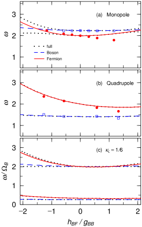
Figure 1: (Color online) The frequencies of the monopole (a) and the quadrupole oscillations (b) in the spherically-symmetric system ($\kappa_{L}=1$) obtained in the scaling method: the co-oscillating (dotted lines, full), the boson-intrinsic (dashed lines), and the fermion-intrinsic (solid lines) modes. The open squares and full circles denote the numerical results obtained in the TDGP+Vlasov calculation for the boson- and fermion-intrinsic frequencies, which are taken from Refs. tomoBF (monopole) and QPBF (quadrupole). In panel (c), the frequencies of the breathing oscillations when $\kappa_{L}=1/6$ obtained in the scaling method are shown.

In the monopole oscillation (a), on the other hand, the frequencies of the boson and fermion intrinsic modes have crossing points at $h_{BF}/g_{BB}\approx-1.5$ and $2.2$ respectively. In the region of $-1.5\lesssim h_{BF}/g_{BB}\lesssim 2.2$, the co-oscillating collective oscillation almost agrees with the intrinsic modes, but, in the region, $h_{BF}/g_{BB}\lesssim-1.5$ and $2\lesssim h_{BF}/g_{BB}$, the frequencies of the co-oscillating modes are different from those of the boson-/fermion-intrinsic modes.

In the same figure, we plot the boson- and fermion-intrinsic frequencies obtained in the TDGP+Vlasov approach (the open squares and the full circles) tomoBF ; QPBF . We find that the scaling method well-reproduces the results in the TDGP+Vlasov approach for the BF attractive interaction, but gives the different values when $h_{BF}/g_{BB}\gtrsim 0$ (monopole oscillation) and $h_{BF}/g_{BB}\gtrsim 1$ (quadrupole oscillation). The similar behavior has also been found in the dipole oscillations tbDPL , and we have explained about this discrepancy in the previous papers tbDPL ; QPBF .

In the last panel (Fig. 1), we show the frequencies when $\kappa_{L}=1/6$. For convenience we refer to the four collective states as state-1 $\sim$ -4 in high-to-low order of their oscillation frequencies; the level crossings are found in the states-1 and -2 at $h_{BF}/g_{BB}\approx 0$ and $1$.

In Fig. 2 we show the components of the eigenvector $\bm{\lambda}$ of the state-1 (1), the state-2 (2), the state-3 (3) and the state-4 (4). From the panels (1) and (2), we find that the state-1 and the state-2 are the transverse modes; when $0\lesssim h_{BF}/g_{BB}\lesssim 1$, the relative phases between the BTB and FTB oscillations are in-phase ($\lambda_{FT}\approx\lambda_{BT}$) for the state-1 and out-of-phase ($\lambda_{FT}\approx-5\lambda_{BT}$) for the state-2. In the other region of $h_{BF}/g_{BB}$ these two states show the exchange of oscillations characters, which originated in this exchange of the level crossing of the frequencies of the state-1 and -2. We call them the in-phase transverse breathing (ITB) and out-of-phase transverse breathing (OTB) modes.

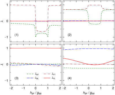
Figure 2: (Color online) Components of the eigenvector of the excited states with the highest excited energies (1), the second highest one (2), the third highest one (3) and the lowest one (4) when $\kappa_{L}=1/6$. The dashed, long-dashed, chain-dotted and solid lines indicate the FTB, FLB, BTB and BLB components $(\lambda_{FT}$, $\lambda_{FL}$, $\lambda_{BT}$, $\lambda_{BL})$.

Fig. 2-(3) shows that the component $\lambda_{FL}$ dominates the eigenvector, so that the state-3 is almost composed of the FLB mode. The eigenvector of the state-4 shows complicates behaviors. From Fig. 2-(4), it is found to be composed of the BLB and BTB modes, and also include the FLB modes when $|h_{BF}|$ is large. When $h_{BF}=0$, the eigen-energy of the state-4 becomes

$$\omega^{2}=\left(1-\frac{v_{B}}{10}\right)\left(2+\frac{3\kappa_{L}^{2}}{2}-\sqrt{4-4\kappa_{L}^{2}+\frac{9\kappa_{L}^{4}}{4}}\right),$$ (42)

with $v_{B}=V_{bb}/X_{B}$. In the limit of large deformation ($\kappa_{L}\ll 1$), it becomes $\omega^{2}\approx 5\kappa_{L}^{2}(1-v_{B}/10)/2$, and the eigenvector of the state-4 is approximated by

$$\left(\begin{array}[]{c}\lambda_{BT}\\ \lambda_{BL}\end{array}\right)\approx\left(\begin{array}[]{c}-1+\frac{10}{17}\kappa_{L}^{2}\\ 4+\frac{5}{34}\kappa_{L}^{2}\end{array}\right)\approx\left(\begin{array}[]{c}-1\\ 4\end{array}\right),$$ (43)

where the bosons oscillates in both the longitudinal and transverse directions in out-of-phase. This mode is similar to the quadrupole oscillation, but the transverse-to-longitudinal amplitude ratio ($-1:4$) is different. According to Ref. Hu04 , we call it the boson axial-breathing (BAB) mode. When $|h_{BF}/g_{BB}|\ll 1$ and $\kappa_{L}\ll 1$, the contribution of the FLB mode can be evaluated in perturbation method:

$$\lambda_{FL}\approx\frac{3V_{3}}{2\mbox{${\tilde{X}}$}_{F}}.$$ (44)

From Eqs. (18), (38) and (44), we find that $\lambda_{FL}<0$ when $0<h_{BF}/g_{BB}<1$, and $\lambda_{FL}>0$ otherwise. The obtained estimation qualitatively agrees with the numerical result (solid line in Fig. 2d).

Thus, the scaling method predict four kinds of collective oscillation modes, ITB, OTB, FLB and BAB modes. In the next section we examine this description in the time-dependent approach.

III Breathing Oscillations in Dynamical Approach

III.1 Time-Dependent Equations

In this section we describe the time evolution of the system using the TDGP equation for the boson condensate and the Vlasov equation for the fermions KB :

$$i\frac{\partial}{\partial\tau}\phi_{c}(\mbox{$\bm{r}$},\tau) = \left\{-\frac{1}{2}\nabla_{r}^{2}+U_{B}(\mbox{$\bm{r}$})\right\}~{}\phi_{c}(\mbox{$\bm{r}$},\tau),$$ (45)

$$\frac{d}{d\tau}f(\mbox{$\bm{r}$},\mbox{$\bm{p}$};\tau) = \left\{\frac{\partial}{\partial\tau}+{\mbox{$\bm{p}$}}\cdot{\nabla_{r}}-[\nabla_{r}U_{F}(\mbox{$\bm{r}$})][\nabla_{p}]\right\}f(\mbox{$\bm{r}$},\mbox{$\bm{p}$};\tau)=0,$$ (46)

where $f(\mbox{$\bm{r}$},\mbox{$\bm{p}$};\tau)$ is the fermion phase-space distribution function, and the $U_{B}$ and $U_{F}$ are effective potentials for bosons and fermions:

$$U_{B}(\mbox{$\bm{r}$}) = \frac{1}{2}(\mbox{$\bm{r}$}_{T}^{2}+\kappa_{L}^{2}z^{2})+g_{BB}\rho_{B}(\mbox{$\bm{r}$})+h_{BF}\rho_{F}(\mbox{$\bm{r}$}),$$ (47)

$$U_{F}(\mbox{$\bm{r}$}) = \frac{1}{2}m_{f}\omega^{2}_{f}(\mbox{$\bm{r}$}_{T}^{2}+\kappa_{L}^{2}z^{2})+h_{BF}\rho_{B}(\mbox{$\bm{r}$}).$$ (48)

In order to solve the Vlasov equation (46) numerically, we use the test-particle method TP ; for each fermion, we prepare ${\tilde{N}}_{T}$ test particles per fermion whose coordinates and momenta are $\mbox{$\bm{r}$}_{i}$ and $\mbox{$\bm{p}$}_{i}$, Then the fermion phase-space distribution function is described as

$$f(\mbox{$\bm{r}$},\mbox{$\bm{p}$},\tau)=\frac{(2\pi)^{3}}{\mbox{${\tilde{N}}_{T}$}}\sum_{i=1}^{{\tilde{N}}_{T}N_{f}}\delta\{\mbox{$\bm{r}$}-\mbox{$\bm{r}$}_{i}(\tau)\}\delta\{\mbox{$\bm{p}$}-\mbox{$\bm{p}$}_{i}(\tau)\}.$$ (49)

Substituting Eq.(49) into Eq.(46), we can obtain the equations of motion for test-particles:

$$\frac{d}{d\tau}\mbox{$\bm{r}$}_{i}(\tau)=\frac{\mbox{$\bm{p}$}_{i}}{m_{f}},\quad\frac{d}{d\tau}\mbox{$\bm{p}$}_{i}(\tau)=-\nabla_{r}U_{F}(\mbox{$\bm{r}$}).$$ (50)

As the initial conditions of time-development at $\tau=0$, we use the boosted condensed-boson wave function and the fermion test-particle coordinates:

$$\phi_{c}(\mbox{$\bm{r}$},\tau=0) = \exp\left\{\frac{i}{2}(b_{T}r_{T}^{2}+b_{L}z^{2})\right\}\phi_{c}^{(g)}(\mbox{$\bm{r}$}),$$ (51)

$$\mbox{$\bm{p}$}_{T}(i)=\mbox{$\bm{p}$}_{T}^{(g)}(i)+m_{f}\omega_{f}c_{T}\mbox{$\bm{r}$}_{T}(i), p_{z}(i)=p_{z}^{(g)}(i)+m_{f}\kappa_{L}\omega_{f}c_{L}z(i),$$ (52)

where $b_{T}$, $b_{L}$, $c_{T}$ and $c_{L}$ are the boost parameters, and the superscript $(g)$ represents the ground state.

In order to examine the aspects of the breathing oscillation, we introduce the quantities:

$$\Delta x_{L,T}(\tau;s)=\frac{1}{2}\left[\frac{R^{2}_{L,T}(\tau;s)}{R_{L,T}^{(g)2}(s)}-1\right]\approx\frac{R_{L,T}(\tau;s)}{R_{L,T}^{(g)}(s)}-1,\quad(s=B,F)$$ (53)

where $R_{L,T}(B)$ and $R_{L,T}$ are the root-mean-square radii of the boson and fermion density-distributions along longitudinal (transverse) directions. We should note that the last approximate term is satisfied when the variation is small: $|R_{L,T}-R_{L,T}^{(g)}|\ll R_{L,T}^{(g)}$. The quantities $\Delta{x}$ represent changes of particle distributions in longitudinal and transverse directions.

In order to inspect the oscillation modes, we use the strength functions defined by the Fourier transform of $\Delta x_{L,T}(s)$ ($s=B,F$):

$$S_{L,T}(\omega;s) = \int^{t_{f}}_{t_{i}}d\tau\Delta x_{L,T}(\tau;s)\sin{\omega\tau}$$ (54)

In actual calculation, we use the test-particle number ${\tilde{N}}=100$ and take $0<\tau<200$ for the integration interval unless otherwise noted.

In the linear-response approximation, only the $S_{L,T}$ have finite strengths in the present initial conditions: $\Delta x_{L,T}=0$ and $d\Delta x_{L,T}/d\tau\neq 0$ at $\tau=0$.

In the present paper, we take three kinds of mixtures: ¹⁷⁰Yb-¹⁷¹Yb ($h_{BF}/g_{BB}=0.573$), ¹⁷⁰Yb-¹⁷³Yb ($h_{BF}/g_{BB}=-1.273$) and ¹⁷⁴Yb-¹⁷³Yb ($h_{BF}/g_{BB}=1.325$), where the boson-fermion interaction is weakly repulsive, strongly attractive and strongly repulsive, respectively; the scattering lengths are shown in Ref.  QPBF .

We deal with the Yb-Yb system, where the number of the bosons and the fermions are $N_{b}=10000$ and $N_{f}=1000$, respectively. The trapping potential parameters are $\Omega_{B}=2\pi\times 300$ (Hz), $\kappa_{L}=1/6$ and $\omega_{f}=1$: these values are chosen to be almost similar with those in the experiment by Kyoto group Fukuhara-M (the axial symmetry is a little broken in the actual experiment). The mass differences of the Yb-isotopes can be safely neglected, so that we use the same mass ($m_{f}=1$) for all Yb-isotopes in the present calculation.

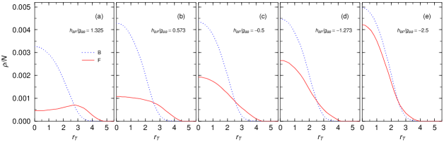
Figure 3: (Color online) The ground-state density distributions of the BF mixtures for $h\equiv h_{BF}/g_{BB}=1.325$ (a), $0.573$ (b), $-0.5$ (c) $-1.273$ (d) and $-2.5$ (e). The (a), (b) and (c) correspond to the ¹⁷⁴Yb-¹⁷³Yb, ¹⁷⁰Yb-¹⁷¹Yb and ¹⁷⁰Yb-¹⁷³Yb mixtures, respectively. The dotted and solid lines represent are for the boson and fermion distributions.

III.2 The Ground States

In Fig. 3, we show the boson (dotted line) and fermion (solid lines) density distributions of the ground states at $z=0$ when $h_{BF}/g_{BB}=1.325$ (¹⁷⁴Yb$-^{173}$Yb) (a), $0.573$ (¹⁷⁰Yb$-^{171}$Yb) (b), $-0.5$ (c), $-1.273$ (¹⁷⁰Yb$-^{173}$Yb) (d) and $-2.5$ (e), where $g_{BB}=0.154$ for Fig. 3a and 0.0964 for the other cases. We should note that the $\omega_{z}z$-dependence of the density distribution at $r_{T}=0$ are approximately the same as these distribution exhibited in this figure because of the scaling invariance discussed in the previous section.

The boson densities are center-peaked in all cases. In contrast, the fermion densities have a surface-peaked shape when $h_{BF}/g_{BB}>1$ (Fig. 3a), but have a center-peaked shape when $h_{BF}/g_{BB}<1$. As the BF interactions becomes attractively stronger ($h_{BF}/g_{BB}<0$), the fermion density is more largely distributed in the boson-distributed regions, and the boson density increases at the center. This BF interaction dependence of the fermion density distribution can be easily explained in the TF approximation, where the ground-state density is determined not by $h_{BF}$ and $g_{BB}$ independently but only through the ratio $h_{BF}/g_{BB}$.

In the limit of the large boson and fermion numbers, the density distribution is well approximated by the results in the TF method: $\rho_{B,F}(\mbox{$\bm{r}$})\approx\rho_{B,F}^{(s)}(\sqrt{\mbox{$\bm{r}$}_{T}+\kappa_{T}^{2}z^{2}})$ with $\rho^{(s)}$ being that in the spherical trap ($\kappa_{L}=1$). The explicit form of $\rho^{(s)}_{B,F}$ have been given in the previous paper QPBF .

III.3 Longitudinal Breathing Oscillations

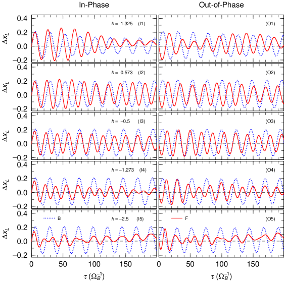
Figure 4: (Color online) Time evolution of longitudinal $\Delta x_{L}(B)$ (boson oscillation, dotted lines) and $\Delta x_{L}(F)$ (fermion oscillation, solid lines) for the in-phase initial condition, $b_{T}=c_{T}=0$ and $b_{L}=c_{L}=0.01$, (left figures) and for the out-of-phase initial condition, $b_{T}=c_{T}=0$ and $b_{L}=-c_{L}=0.01$, (right figures). The panels from the upper to the lower columns are for $h\equiv h_{BF}/g_{BB}=1.325$ (I1 & O1), $0.573$ (I2 & O2), $-0.5$ (I3 & O3), $-1.273$ (I4 & O4) and $-2.5$ (I5 & O5), respectively.

First, we present numerical calculations in the TDGP+Vlasov approach with the longitudinally-deformed BF in-phase condition, $b_{T}=c_{T}=0$ and $b_{L}=c_{L}=0.01$. We note that this condition is consistent with the actual experiments by Kyoto group Fukuhara-M . For comparison, we also present the BF out-of-phase condition, $b_{T}=c_{T}=0$ and $b_{L}=c_{L}=0.01$.

In Fig. 4, we show the time-dependence of $\Delta x_{L}$ for $h_{BF}/g_{BB}=1.325$, $0.573$, $-0.5$, $-1.273$ and $-2.5$. The left and right figures exhibit the results for the in-phase and out-of-phase initial conditions. The $\Delta x_{L}(B)$ is found to oscillate monotonously (dotted lines), while the $\Delta x_{L}(F)$ shows a small damping and/or a small beat. Furthermore, we can find that the $x_{L}(F)$ has a tendency to synchronize with $x_{L}(B)$ in the case of the large BF couplings ($h_{BF}/g_{BB}\geq 1.0$), and that the $x_{L}(F)$ gradually increases in $\tau\gtrsim 150$ when $h_{BF}/g_{BB}\geq 2.5$.

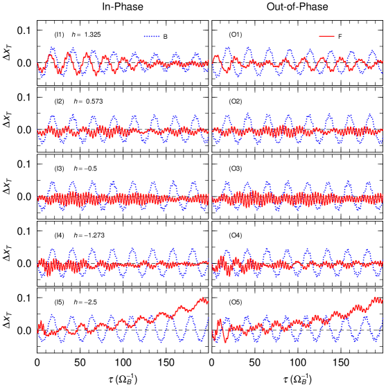
Figure 5: (Color online) Time evolution of transversal $\Delta x_{T}(B)$ (boson oscillation, dotted lines) and $\Delta x_{T}(F)$ (fermion oscillation, solid lines) in the longitudinal oscillations. The other conditions are the same as those in Fig. 4.

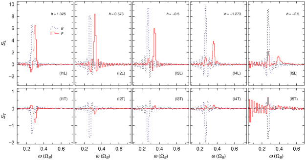
Figure 6: (Color online) The longitudinal (upper figures) and transverse strength functions (lower figures) of boson $S_{L,T}(B)$ (dotted lines) and fermion $S_{L,T}(F)$ (solid lines) (solid lines) for the in-phase initial conditions. The result of each panel correspond to the oscillation shown in the left figures of Fig. 4

In Fig. 5, we show the time-dependence of $\Delta x_{T}$ in the same oscillations with Fig. 4. The boson $\Delta x_{T}(B)$ (dotted lines) monotonously oscillate with the same period with $\Delta x_{T}(F)$, but out of phase. The fermion $\Delta x_{T}(F)$ seems to be a superposition of two modes with different periods (dotted lines), which makes a beat. The long-period mode is dominant when $|h_{BF}/g_{BB}|\gtrsim 1$, while the short-period mode becomes dominant when $|h_{BF}/g_{BB}|\lesssim 1$. Furthermore, in the case of the strongly attractive BF interaction ($h_{BF}/g_{BB}=-2.5$,I5 & O5), monotonous increases of $x_{T}(B)$ are confirmed in $\tau\gtrsim 100$, which means the fermion-gas expansions in the transverse direction.

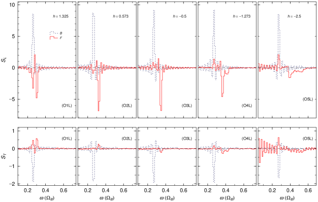
Figure 7: (Color online) Same as Fig. 6, but the initial condition is out-of-phase. The longitudinal (upper figures) and transverse strength functions (lower figures) of boson $S_{L,T}(B)$ (dotted lines) and fermion $S_{L,T}(F)$ (solid lines) (solid lines) for the in-phase initial conditions. The result of each panel correspond to the oscillation shown in the right figures of Fig. 4.

We show the longitudinal (upper panels) and transverse strength functions (lower panels) of the longitudinal oscillations for the in-phase (Fig. 6) and the out-of-phase (Fig. 7) initial conditions in $h_{BF}/g_{BB}=1.325$ (I1), $0.573$ (I2), $-0.5$ (I3), $-1.273$ (I4) and $-2.5$ (I5).

First, we find that the $S_{L}(B)$ (dotted lines) and $S_{T}(B)$ (dashed lines) have one large peak at almost the same frequency $\omega\approx 0.26-0.27$ in all mixtures. The peak height ratios are $-S_{L}(B)/S_{T}(B)\approx 4.7$ (I1 & O1), $5.33$ (I2 & O2), 4.8 (I3 & O3), 4.8 (I4 & O4), 5.31 (I5 & O5), and almost independent of the initial condition. In addition, these ratios approximately agree with the result obtained in the scaling method for the BAB mode, $\lambda_{BL}/\lambda_{BT}\approx-4$.

On the other hand, the $S_{L}(F)$ show two peaks; one peak appears at the same frequency with the peak of $S_{L}(B)$, and the strengths $S_{L}(F)$ at the first peaks are positive/negative for the attractive/repulsive BF interaction. Clearly the mode corresponding to the first peak is the forced oscillation caused by the boson oscillation as shown in the dipole tbDPL and quadrupole QPBF oscillations. The similar behavior is appeared in the $\lambda_{FL}$ of the BAB mode in the scaling method in Eq. (44).

The strengths at the second peak become positive/negative for the in-phase/out-of-phase initial conditions, and the boson oscillations show no strengths there. In addition, we should note that $S_{T}(F)/S_{L}(F)<0$ when $h_{BF}/g_{BB}>0$ and $S_{T}(F)/S_{L}(F)>0$ when $h_{BF}/g_{BB}<0$; these behaviors are the same as those of $\lambda_{FT}/\lambda_{FL}$ in the FLB mode in the scaling method (see Fig. 2-(3)). So this mode is the intrinsic fermion oscillation mode corresponding to the FLB mode predicted in the scaling method.

Thus, the qualitative behavior of the longitudinal oscillation almost agrees with the collective modes predicted in the scaling method except the sign of $S_{L}(F)$ in the BAB modes; in the scaling method $\lambda_{BL}$ and $\lambda_{FL}$ have the same sign when $h_{BF}/g_{BB}\gtrsim 1.0$.

The other difference from the results in the scaling method is the fermion gas expansions mainly in the transverse directions in the case of strongly attractive BF-interaction, which we discuss in the next subsection.

III.4 Transverse Breathing Oscillations

In this subsection, we discuss the oscillations caused by the transversely-deformed initial conditions, $b_{T}=c_{T}=0.1$ and $b_{L}=c_{L}=0$ (BF-in-phase condition), and $b_{T}=-c_{T}=0.1$ and $b_{L}=c_{L}=0$ (BF-out-of-phase condition).

In Fig. 8, we show the time-dependence of $\Delta x_{T}$ for $h_{BF}/g_{BB}=1.325$, $0.573$, $-0.5$, $-1.273$ and $-2.5$. The left and right figures exhibit the results with the in-phase and out-of-phase initial conditions, respectively. The $\Delta x_{T}(B)$ is found to oscillate monotonously (dotted lines), while the $\Delta x_{T}(F)$ shows a small damping and/or a small beat.

These oscillations also excite the longitudinal-oscillation modes of very small amplitudes. They are not synchronized with the transverse oscillations, and their qualitative behavior is the same as the oscillation modes discussed in the previous section.

We find that the oscillations with the in-phase initial condition is monotonous, and those with the out-of-phase initial condition show a beat in early stage of time and become monotonous in the latter stage of time, where relative phases between boson and fermion oscillations become in-phase. In addition, the positive shifts of the mean values appear in $\Delta x_{T}$ for the out-of-phase initial conditions.

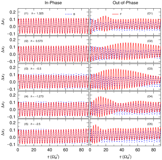
Figure 8: (Color online) Time evolution of transversal $\Delta x_{T}(B)$ (boson oscillation, dotted lines) and $\Delta x_{L}(F)$ (fermion oscillation, solid lines) for the in-phase initial condition, $b_{T}=c_{T}=0.1$ and $b_{L}=c_{L}=0$, (left figures) and. for the out-of-phase initial condition, $b_{T}=-c_{T}=0.1$ and $b_{L}=c_{L}=0$ (right figures). The panels from the upper to the lower columns are for $h\equiv h_{BF}/g_{BB}=1.325$ (I1 & O1), $0.573$ (I2 & O2), $-0.5$ (I3 & O3) $-1.273$ (I4 & O4) and $-2.5$ (I5 & O5), respectively.

In Fig. 9 we show the same oscillations in the later time, $\tau\geq 115$. We can confirm clearly the relative in-phases behaviors between the boson and fermion oscillations and the positive shift of the mean values of $\Delta x_{T}$. Furthermore, we find the expansion of the fermion gases for the transverse direction, which has been shown also in the longitudinal oscillations. In Fig. 9 the fermion gas expansions appear moderately for $h_{BF}/g_{BB}=-2$ and remarkably in the BF mixtures of the strongly attractive BF interactions ($h_{BF}/g_{BB}=-2.5$) but, in the case of the weak interactions ( $h_{BF}/g_{BB}=-1.273$), no expansions are observed at least in the time intervals of $\tau\geq 115$.

In order to examine the oscillation behaviors, we show the transverse strength functions $S_{T}$ in Fig 10. In all cases of the in-phase and out-of-phase initial conditions and of the BF interactions, the boson and fermion strength functions, $S_{T}(B)$ and $S_{T}(F)$, have one sharp peak at the same frequencies, and $S_{T}(B)\approx S_{T}(F)$ at the peaks. Furthermore, a broad peak exists in every oscillation for the out-of-phase initial condition; the $S_{L}(B)$ and $S_{T}(B)$ take opposite values in the peak area and the width becomes large as $|h_{BF}/g_{BB}|$ increases.

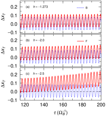
Figure 9: (Color online) Time evolution of $\Delta x_{T}(B)$ (boson oscillation, dotted lines) and $\Delta x_{T}(F)$ (fermion oscillation, solid lines) for the in-phase initial condition. The panel (a), (b) and (c) are for $h\equiv h_{BF}/g_{BB}=-1.273$, $-2.0$ and $-2.5$.

The present behaviors of the transverse oscillations can be explained from the superposition of the ITB and OTB oscillation modes; the strengths of the ITB modes concentrates on the narrow energy region, and $S_{T}(B)$ and $S_{T}(F)$ have the almost same values, while the strengths of the OTB modes distribute in broad energy region, and is dominant in the fermion strength function. The ratios between $S_{T}(B)$ and $S_{T}(F)$ are qualitatively similar to those of $\lambda_{BT}$ to $\lambda_{FT}$ obtained in the scaling method.

The narrow ITB and broad OTB peaks explain the behaviors of $\Delta x_{T}(B)$ and $\Delta x_{T}(F)$ observed in Figs. 10. When the relative phase between the boson and fermion oscillations is in-phase at the initial time, the oscillation starts only with the ITB mode, which is monotonous. But, for the out-of-phase initial conditions, the oscillation includes the ITB and OTB modes at the beginning, which causes a beat phenomenon in the $\Delta x_{T}(F)$ in early stage of time. Then, the OTB modes damps rapidly, the transverse oscillation becomes monotonous and relatively in-phase between the boson and fermion oscillations.

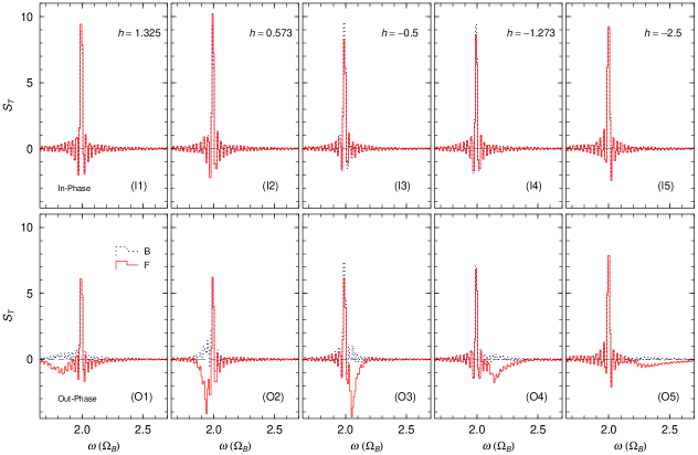
Figure 10: (Color online) Strength Functions of the transverse strength functions for the boson (dotted lines) and fermion oscillations (solid lines) for the in-phase initial condition (upper figures) and for the out-of-phase initial conditions (lower figures) with $h\equiv h_{BF}/g_{BB}=1.325$ (I1 & O1), $=0.573$ (I2 & O2), $=-0.5$ (I3 & O3), $=-1.273$ (I4 & O4) and $=-2.5$ (I5 & O5).

As shown before, the OTB mode has very small boson strength, so that we can consider it as a fermion intrinsic mode. In Fig. 11, we show the time evolution of $\Delta x_{T}(F)$ when the boson motion is frozen. The dampings are more rapid for $h_{BF}/g_{BB}=1.325$ (a) and $-1.273$ (c) than that for $h_{BF}/g_{BB}=0.573$ (b). The effective potentials for fermion are close to the harmonic oscillator one in weak BF interactions and gives very slow dampings of the fermion oscillation, but the potentials for the strong BF interaction causes rapid damping effect through their large anharmonicities. In the bottom panel Fig. 11-(d), the calculation is shown for $h_{BF}/g_{BB}=-1.273$ with the initial amplitude twice larger than in panel (c); we find the shift of the equilibrium positions of oscillation in the outward direction larger than in panel (c). It shows that the slight shift of the equilibrium positions of oscillation in $\Delta x_{T}$ in the case of the out-of-phase initial condition is caused by the energy transfer from boos gas to fermions through the process of the damping of the OTB mode.

In our previous studies of the BF mixtures in the spherical traps tbDPL ; QPBF , the oscillations can be described by the superposition of the boson and fermion intrinsic modes. In the present calculation in the time-dependent approach, we find a phenomenon that these intrinsic modes are coupled and appear as the in-phase and out-of-phase intrinsic modes. In the quadrupole oscillations with the spherical trap, furthermore, the relative phase between the boson and fermion oscillations becomes in-phase or out-of-phase at the later stage of time corresponding to the attractive or repulsive boson-fermion interactions QPBF ; in contrast, the relative phase in the monopole oscillations are in-phase independently of the BF interactions MSY1 .

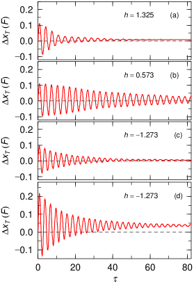
Figure 11: (Color online) Time evolution of $\Delta x_{T}(F)$ in the case of frozen boson motions with the transversal initial conditions: $c_{L}=0$ and $c_{T}=0.1$ for the panel (a-c) and $c_{L}=0$ and $c_{T}=0.2$ for the panel (d). The BF interactions are $h\equiv h_{BF}/g_{BB}=1.325$ (a), $0.573$ (b), $-1.273$ (c,d).

In the spherical trap, the region of increasing boson density are close to that of decreasing density in the dipole and quadrupole oscillations. In these cases, the fermions easily move from the dense region to the dilute region of the boson density when the BF-interaction is repulsive. In the monopole oscillation, on the other hand, change of the boson density occurs uniformly. In fact the relative phase between the boson and fermion oscillations is not definite and depends on the strength of the BF interaction and the boson/fermion numbers et. al.

In the largely prolate deformed trap, expansions and shrinks of the fermion density occurs easily in the transverse direction in the case of the longitudinal breathing oscillations, but such an anisotropy of the fermion flow is difficult in the transverse breathing oscillations. Thus, in the largely deformed trap, the longitudinal and transverse breathing oscillations show the similar behaviors with the quadrupole and monopole ones in the spherical trap, respectively.

Furthermore, the fermion-gas expansion in the case of strongly attractive BF-interactions has also appeared in the quadrupole oscillation in the spherical trap QPBF though this mode is time-even. In the spherical trap, this expansion is a part of the monopole oscillation, which is decoupled from the quadrupole oscillation and not included at the beginning. In contrast, in the largely deformed trap, the expansion mode is a part of the FLB oscillation, which is coupled with the other modes, so that this expansion appears also in time-odd modes. Indeed, the expansion mode appears in the monopole oscillation with the time-even initial condition in the spherical trap when the initial condition is taken to be time-odd.

III.5 Comparison with the Scaling Method

In this subsection, we discuss the BF-interaction dependence of the intrinsic-mode frequencies obtained in the TDGP+Vlasov approach, and compare them with those in the scaling method.

As discussed in Sec. II, the breathing oscillations of the BF mixtures are described as the superposition of four collective modes: BAB (boson axial-breathing), FLB (fermion longitudinal breathing), ITB (in-phase transverse breathing) and OTB (out-of–phase transverse breathing), which are characterized in the scaling method. Fig. 12 shows the $h_{BF}/g_{BB}$-dependences of the boson and fermion intrinsic frequencies, which are obtained from the peak positions of the strength functions.

The excitation energies of the BAB and ITB modes in TDGP+Vlasov agree with those of the state-1 and state-3 in the scaling method, respectively. As discussed in the previous subsections, the mixing ratios of the boson and fermion intrinsic modes in these states are also qualitatively same in two approach, but the excitation energies of the FLB and OTB (FTB) modes dose not agree.

The peaks of the strength functions corresponding to the BAB and ITB modes are narrow, and their strengths concentrate into one mode. In contrast, the OTB peak is very broad in any condition, and the corresponding oscillation damps very rapidly. In addition, the peak correspond to the FLB mode is also broad when $h_{BF}/g_{BB}\lesssim-1.0$. Thus, the strength of the fermion oscillation modes do not concentrate to one mode with the fixed frequency, and this oscillation behavior is not applicable in the scaling method based on the sum-rule approach.

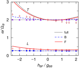
Figure 12: (Color online) Intrinsic frequencies of the breathing oscillations of the boson and fermion gases obtained in the TDGP+Vlasov approach; full squares, open circles, solid triangle and open diamonds are for the BAB, FLB, ITB and OTB modes in the mixtures, respectively. Solid, dashed and dotted lines represent the results in the scaling method (same as Fig. 1c).

Furthermore, when the boson motion is frozen, the intrinsic frequency of the FLB oscillation in the scaling method is written as

$$\omega_{FLB}^{2}=\frac{\int d^{3}r\rho_{F}(\mbox{$\bm{r}$})\left(3z^{2}\frac{\partial^{2}U_{F}}{\partial z^{2}}+5\frac{\partial U_{F}}{\partial z}\right)}{2m_{f}\int d^{3}rz^{2}\rho_{F}(\mbox{$\bm{r}$})},$$ (55)

where $U_{F}$ is the fermion potential defined as Eq. (48). Thus, the oscillation frequency is reflected by the first and second derivative of fermion potentials.

In the scaling method, the amplitude of the oscillation is assumed to be very small, and the $\omega_{FLB}$ is reflected by the potential shape in the region where the fermions occupy. When the amplitude becomes larger, however, the $\omega_{L}$ is influenced from the potential shape outside the fermion occupation region, and its value approaches to $2\kappa_{L}\omega_{f}=0.333$. The FTB oscillation also shows similar behavior, and its frequency approaches $2\omega_{f}=2$ as the amplitude becomes larger.

The frequencies of the fermion intrinsic oscillation modes monotonously decrease as the $h_{BF}/g_{BB}$ becomes larger in the TDGP+Vlasov approach though the frequencies decrease when $h_{BF}/g_{BB}\lesssim 0.5$ and increase $h_{BF}/g_{BB}\lesssim 0.5$ in the scaling method. This behavior of the fermion frequencies comes from the structure change of the fermion ground-state density distribution into the surface-peaked shape (Fig. 3).

In the scaling method calculation, the frequency of the FLB and FTB (OTB) mode has the minimum around $h_{BF}/g_{BB}\sim 0.5$, and increases with increase of $h_{BF}/g_{BB}$ in the region of $h_{BF}/g_{BB}>1$ (Fig. 12, solid line); On the other hand, in the TDGP+Vlasov approach, the density distribution and the velocity field varies in time in large amplitude oscillations. In the mixture of $h_{BF}/g_{BB}>1$, the minimum position of the fermion potential is on the spherical surface at the border of the boson density distribution, and the fermion gas oscillates around this surface; it results in the frequencies of the fermion modes smaller than those obtained in the sum-rule. The same discrepancies appears in the dipole and quadrupole oscillations in the spherical traptomoBF ; monoEX ; tbDPL ; QPBF .

Finally, we comment on the experiment by Fukuhara et.al. in Ref. Fukuhara3 , where the frequencies of the BLB oscillations was obtained. The experimental results show that $\omega_{BAB}=1.69\kappa_{L}\Omega_{B}$ when $h_{BF}/g_{BB}=0$ and $1.67\kappa_{L}\Omega_{B}$ when $h_{BF}/g_{BB}=1.325$ (¹⁷⁴Yb-¹⁷³Yb ), while the present calculations are $\omega_{BAB}=1.59\kappa_{L}\Omega_{B}$ for $h_{BF}/g_{BB}=0$ and $1.57\kappa_{L}\Omega_{B}$ for $h_{BF}/g_{BB}=1.325$. The experiments have been performed using the non-axial symmetric trap with the different atomic numbers at finite temperature. Then, we cannot make direct comparison between the two results, but we can mention that the two results qualitatively agree each other, particularly in the 1.2% increase when the BF coupling is varied from $h_{BF}/g_{BB}=0$ to $h_{BF}/g_{BB}=1.325$.

IV Summary

In this paper, we investigated the collective breathing oscillation of the BF mixtures of Yb isotopes in the deformed trap ($\kappa_{L}=1/6$) by varying the BF-coupling constant.

The scaling method predicts that the couplings between BLB and BTB modes and between the BTB and FTB modes make four intrinsic modes, BAB, FLB, ITB and OTB modes. This prediction is qualitatively consistent with the results in the TDGP+Vlasov approach.

In the case of the weak boson-fermion interactions, the longitudinal and transverse breathing oscillations decouple in the largely deformed trap of prolate shape. Because of the large interaction energy coming from the condensed bosons, the boson breathing oscillations couple into the intrinsic BTB and BAB modes, and the intrinsic FTB and FLB modes are made from the fermion oscillations. The actual time-development processes are described by the superposition of these intrinsic modes.

The intrinsic transverse modes (BTB & FTB) have very close frequencies, and it is similar in the longitudinal modes (BAB & FLB); the frequencies of these two pairs separate very well.

In the spherical trap, the fermion oscillation have been shown to have the boson-forced oscillation modes and the two intrinsic modes which correspond to the inside- and outside-fermion oscillations for the boson-distributed regions. In the present prolate deformed trap, no outside-fermion modes appear.

In the longitudinal breathing oscillations a beat and a small damping appear for both the boson an fermion oscillations though the boson oscillations shows these behaviors much weaker than the fermion oscillation. The intrinsic frequencies of the BAB and FLB modes are very close, and the influence from the boson oscillation to the fermion oscillation is large while the opposite influence is weak. The FLB oscillation includes the two mode with the close frequencies and show the above behaviors.

The transverse breathing oscillations show monotonous behavior when the initial condition is in-phase though the oscillation behavior is a little complex in the case of the out-of-phase initial condition. In the fermion transverse breathing oscillations, we found that the fermion-gas frequencies vary in time and converges into the same frequencies with the boson oscillations and the relative phases of the boson and fermion oscillations become in-phase. This phenomenon are shown to be explained by dampings of the intrinsic fermion modes when the boson motion is frozen.

In the case of the strongly-attractive boson-fermion interaction, $h_{BF}/g_{BB}\lesssim 2$, the expansion of fermi gas occurs in the transverse direction. When the BF coupling is attractively large, most of fermions populate inside the boson region of the ground state. The boson gas oscillation heats the fermi gas and run the fermion out from the boson occupied region, so that the fermi gas is expanded. Such a behavior is beyond that in the linear response theory and also beyond our approach.

These results show that the longitudinal breathing oscillations in the largely deformed trap are similar with the quadrupole ones in the spherical trap QPBF . In contrast, the transverse breathing oscillations correspond to the monopole ones in the two dimensional system; it is the similar property of the monopole oscillation in the three dimensional system.

In this paper we discuss the collective oscillations of the BF mixtures of Yb isotopes at $T=0$. The actual experiments have been done at finite temperatures Fukuhara3 ; Fukuhara-M . In addition we need to examine the heating of the bose gas as mentioned above. Thus thermal bosons should give some contributions; the introduction of such effects into the present approach through two-body collision terms JackZar ; BUU1 should be done also in the future.

Acknowledgement

This work is supported in part by the Japanese Grand-in-Aid for Scientific Research Fund of the Ministry of Education, Science, Sports and Culture (21540212 and 22540414).

References

-
(1)
E.A. Cornell and C.E. Wieman, Rev. Mod. Phys. 74, 875 (2002);
W. Ketterle, Rev. Mod. Phys. 74, 1131 (2002). - (2) F. Dalfovo, et al., Rev. Mod. Phys. 71, 463 (1999).
- (3) C.J. Pethick and H. Smith, ”Bose-Einstein Condensation in Dilute Gases”, Cambridge University Press (2002).
- (4) J.O. Andersen, Rev. Mod. Phys. 76, 599 (2004).
- (5) A.G. Truscott, K.E. Streker, W.I. McAlexander, G.B. Partridge and R.G. Hulet, Science 291, 2570 (2001).
- (6) G. Rotor, F. Riboli, G. Modugno and M. Inguscio, Phys. Rev. Lett. 89, 150403 (2002).
-
(7)
B. DeMarco and D.S. Jin, Science 285, 1703 (1999);
S.R. Granade, M.E. Gehm, K.M. O’Hara, J.E. Thomas, Phys. Rev. Lett. 88, 120405 (2002). - (8) F. Schreck, et al., Phys. Rev. Lett. 87, 080403 (2001).
- (9) Z. Hadzibabic, et al., Phys. Rev. Lett. 88, 160401 (2002); ibid 91, 160401 (2003).
- (10) M. Modugno, F. Ferlaino, F. Riboli, G. Roati, G. Modugno, M. Inguscio, Science 297, 2240 (2002); Phys. Rev. A 68, 043626 (2003).
- (11) H. Feshbach, Ann. Phys. (NY) 19, 287 (1962).
- (12) K. Mølmer, Phys. Rev. Lett. 80, 1804 (1998).
- (13) M. Amoruso, A. Minguzzi, S. Stringari, M. P. Tosi and L. Vichi, Eur. Phys. J. D 4, 261 (1998).
- (14) M.J. Bijlsma, B.A. Heringa and H.T.C. Stoof, Phys. Rev. A 61, 053601 (2000).
- (15) L. Vichi, M. Inguscio, S. Stringari, and G.M Tino, Eur. Phys. J. D 11, 335 (2000).
- (16) L. Vichi, M. Inguscio, S. Stringari and G.M. Tino, J. Phys. B: At. Mol. Opt. Phys. 31 L899 (1998).
- (17) T. Miyakawa, K. Oda, T. Suzuki and H. Yabu, J. Phys. Soc. Japan 69, 2779 (2000).
- (18) N. Nygaard and K. Mølmer, Phys. Rev. A 59, 2974 (1999).
- (19) X.X. Yi and C.P. Sun, Phys. Rev. A 64, 043608 (2001).
- (20) L. Viverit, C.J. Pethick and H. Smith, Phys. Rev. A 61, 053605 (2000).
- (21) P. Capuzzi and E.S. Hernández, Phys. Rev. A 66, 035602 (2002).
- (22) P. Capuzzi, A. Minguzzi and M.P. Tosi, Phys. Rev. A 68, 033605 (2003).
- (23) T. Miyakawa, T. Suzuki and H. Yabu, Phys. Rev. A 64, 033611 (2001).
- (24) R. Roth and H. Feldmeier, Phys. Rev. A 65, 021603(R) (2002).
- (25) P. Capuzzi and E. S. Hernández, Phys. Rev. A 64, 043607 (2001).
-
(26)
T. Sogo, T. Miyakawa, T. Suzuki and H. Yabu, Phys. Rev. A66, 013618 (2002);
T. Sogo, T. Suzuki and H. Yabu, Phys. Rev. A68, 063607 (2003). - (27) T. Miyakawa, T. Suzuki and H. Yabu, Phys. Rev. A 62, 063613 (2000).
- (28) A. Minguzzi and M.P. Tosi, Phys. Lett. A 268, 142 (2000).
- (29) S.K. Yip, Phys. Rev. A64, 023609 (2001).
- (30) T. Maruyama, H. Yabu and T. Suzuki, Phys. Rev. A72, 013609 (2005).
- (31) T. Maruyama, H. Yabu and T. Suzuki, Lazer Physics, 15, 656 (2005).
- (32) T. Maruyama and G.F. Bertsch, Phys. Rev. A77, 063611 (2008)
- (33) T. Maruyama and H. Yabu, Phys. Rev. A80, 043615 (2009).
- (34) Y. Takasu, et al., Phys. Rev. Lett. 91, 040404 (2003).
- (35) T. Fukuhara, S. Sugawa, and Y. Takahashi, Phys. Rev. A76, 051604(R) (2007).
- (36) T. Fukuhara, Y. Takasu, M. Kumakura and Y. Takahashi, Phys. Rev. Lett. 98, 030401 (2007).
- (37) K. Enomoto, M. Kitagawa, K. Kasa, S. Tojo and Y. Takahashi, Phys. Rev. Lett. 98, 203201 (2007); M. Kitagawa, et.al., Phys. Rev. A77, 012719 (2008).
- (38) T. Fukuhara, et al., Appl.Phys. B96, 271 (2009).
- (39) T. Fukuhara, master thesis, Kyoto University, Kyoto (2009).
-
(40)
G.F. Bertsch, Nucl. Phys. A249, 253 (1975);
D.M. Brink and Leobardi, Nucl. Phys. A258, 285 (1976). -
(41)
G.F. Bertsch and K. Stricker, Phys. Rev. C13, 1312 (1976);
T. Suzuki, Prog. Theor. Phys. 64, 1627 (1980). - (42) T. Maruyama and G.F. Bertsch, Phys. Rev. A73, 013610 (2006).
- (43) T. Maruyama and T. Nishimura, Phys. Rev. A75, 033611 (2007).
- (44) L.P. Kadanoff and G. Baym, “Quantum Statistical Mechanics” (1962), NewYork.
- (45) L. Vichi and S. Stringari, Phys. Rev. A60, 4734 (1999).
- (46) O. Bohigas, A.M. Lane and J. Martorell, Phys. Rep. 51, 267 (1979),
- (47) Y. Castin and R. Dun, Phys. Rev. Lett. 77, 5315 (1996).
- (48) M.-O. Mewes, et al., Phys. Rev. Lett. 77, 988 (1996).
- (49) Y. Kagan, E.L. Surkov and G.V. Shlyapnikov, Phys. Rev. A54, R1753 (1996).
- (50) V. Gritsev, P. Barmettler and E. Demler, New J. Phys. 113005 (2010)
- (51) A. del Campo, Phys. Rev. A84, 031606R (2011).
- (52) H. Hu, A. Minguzzi, X.J. Liu and M.P. Tosi, Phys. Rev. Lett., 93, 190403 (2004).
-
(53)
R.W. Hockney and J.W. Eastwood, ”Computer simulations using particles”,
McGraw-Hill, New York, 1981;
C.Y. Wong, Phys. Rev. C25, 1460 (1982). - (54) B. Jackson and E. Zaremba, Phys. Rev. A66, 033606 (2002).
- (55) G.F. Bertsch and S. Das Gupta, Phys. Rep. 160 (1988) 189.