Influence of changing environment on

Shennan-type evolution of stone-age cultural innovation

F.W.S. Lima* and Dietrich Stauffer**

* Departamento de Física, Universidade Federal do Piauí, 64.049-550 Teresina, Piauí, Brazil

** Laboratoire PMMH, École Supérieure de Physique et de Chimie Industrielles, 10 rue Vauquelin, F-75231 Paris, France

visiting from Institute for Theoretical Physics, Cologne University, D-50923 Köln, Euroland

The computer simulations of Shennan (2001) are complemented by assuming the environment to change randomly. For moderate change rates, fitness optimisation through evolution is still possible.

Keywords: Evolution theory, stone age, cultural innovation, computer simulation

Shennan (2001), based on a biological model of Peck et al (1997), showed that in large populations, evolution in a computer model can evolve to a higher average fitness than in a smaller population. This influence of demography may be relevant for an easier spread cultural innovation in homo sapiens $10^{4}\dots 10^{5}$ years ago. Now we test whether this effect survives if the environment changes and if thus also the combination of optimal traits giving the highest fitness changes continuously during the evolution.

Each individual $j$ in the Shennan model has $L$ traits $x_{ij}$ with real numbers $-\infty<x_{ij}<\infty$ and deviations $d_{ij}={\rm abs}(x_{ij}-e_{i})$ from the optimal values $e_{i}$. The fitness or fertility is

$$w_{j}=\exp[-\sum_{i=1}^{L}\;d_{ij}]\quad.$$

We start the simulations with all $e_{i}=x_{ij}$ (Shennan (2001) set all $e_{i}$ to zero permanently). Then at each sweep through the population of $N$ individuals (constituting one time step or generation), each individual $j$ gives birth to one offspring (baby, pupil) with probability $w_{j}$, while with probability $1-w_{j}$ instead the best-fitted individual produces one offspring. Thereafter, all adults die, and the offspring become the new adults. The selection of the best-fitted, instead of any other, individual avoids the extremely low and perhaps unrealistic fitnesses of Shennan’s simple model and follows the spirit of his oblique transmission of culture by teachers instead of parents. Also, at each time step each individual has one randomly selected $x$-value changed by an amount taken randomly between $\pm 0.04$, which represents a useful or damaging innovation, simpler than Shennan (2001) and Peck et al (1997).

The highest curve in our upper figure shows for $L=100$ the resulting fitness, averaged over all individuals and then over the second half of all time steps (geometric mean over the population, arithmetic mean over time). As in Shennan (2001), larger populations are seen to lead to larger overall fitness.

Now as a new aspect in the spirit of Cebrat et al (2009) we introduce a changing environment by changing, with probability $R$ at each time step, also all optimal values $e_{i},\;i=1,2,\dots L$ by random amounts also inhomogeneously distributed between $\pm 0.08$. For example, in the migration of homo sapiens the techniques to walk on snow and ice became helpful only rather late, while dark skin became disadvantageous in the Arctic (see also Gibbons 2010).

Our figure shows reasonable reductions of the fitness for small $R$ while for $R>0.01$ not much is left. Thus for survival, environmental change rates should be not higher than the innovation rate per individual, which is $1/L=0.01$ according to our above rule and our choice $L=100$. Indeed, in the lower part of the figure for $L=10$, we got reasonable survival even for $R=1$. Fig. 2a shows more systematically the dependence on $L$ for larger $L$.

For sexual reproduction, as in Peck et al (1997), we divide the population into men and women; now the two fittest members of the population give birth if they happen to be of different sex. Each of the $L$ traits of the child is randomly selected from father or from mother, with probability 1/2 each. The results are shown in Fig.2b.

Children learn not only from their parents (vertical transmission) but also from biologically unrelated adult teachers (oblique transmission). For the latter case we replace the parent (asexual case) or one of the parents (sexual case) by a randomly selected teacher from whom the child learns half of the traits. Fig.3 shows this oblique transmission; for the sexual case a surprising minimum near $L=2500$ appears for some $R$; Fig.3c shows the results for $R=0.001$ on a logarithmic scale.

We checked with numerous different random number seeds the gap at $L=3500$ in this minimum of Fig.3c as a function of time. We found that for short times the fitness equilibrates to $0.86\pm 0.02$, and then jumps down to (nearly) zero. The jump time varies from 4 to several thousand. This behaviour is similar to homogenous nucleation in metastable states, as for example in supersaturated water vapour. The direction of this rapid transition is, however, opposite to the rapid improvement in human civilisation about 45,000 years ago (Owen et al 2009). (For other $L$ between 150 and 25,000 the results usually are more smooth).

This simulation was triggered by the course of Prof. S. L. Kuhn at Cologne University, winter term 2009/10, where the Shennan paper was read. We thank Profs. Shennan, J. Richter and P.M.C. de Oliveira for encouragement and suggestions, and CNPq for support of the Brazilian author.

Appendix

Two variants of the above asexual model have also been investigated: Instead of the above one innovation per person at each iteration, one may have one innovation for each of the $L$ traits of each person at each iteration (“per person” or “per trait”). And instead of the fitness being exp($-D$) for one person, one may take it as exp($-D/L$), i.e. “with” instead of “without” division. All four combinations are shown in the last figure:

per trait, without: +

per trait, with: x

per person, with: stars

per person, without: squares

the last one being the above standard case. These symbols refer to a population of 1000 at an environmental change rate of 0.003. Thus per trait instead of per person decreases the fitness, and with division by $L$ quite trivially the fitness strongly increases. With a rate 0.3 and a ten times larger population, the two overlapping lines in the figure are obtained, showing that per person or per trait does not matter much for this higher change rate.

If the division by $L$ is applied to the gap in Fig.3c for oblique sexual transmission, then the fitness stays near 0.98 for $L$ between 1000 and 5000, with no gap.

Finally we let the population size fluctuate by a Verhulst factor, instead of keeping it constant, for the standard case “per person” and “without division”. Thus for each of the 10,000 iterations we went again through each individual and let it die with probability $N/K$ where $n$ is the current population and $K=1000$ is usually called the carrying capacity. If the individual survives this “logistic” danger, it produces one additional offspring. We found that the actual populations fluctuate near $K/2$ and that about half of them die out before the 10,000 iterations are finished, if $K$ is about 16 (and $L$ is 10 or 100, for $R$ between 0.001 and 1; $L=1000$, 10,000 and 100,000 for $R=0.003$ only.) Thus random fluctuations will hardly kill a population of more than a dozen individuals. Note that we include also the dangers from the random changes in the environment, but not catastrophes like volcano eruptions not described by our rather smooth environmental changes.

Figure 1: Variation of average fitness with population size, for environmental change rates $R$ increasing from top to bottom. ($10^{4}$ time steps.) Upper part $L=100$, lower part $L=10$.

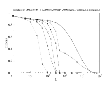
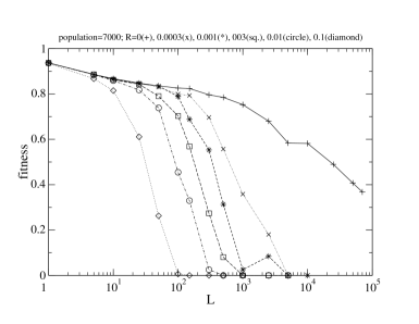
Figure 2: Variation with the number $L$ of traits. Part a shows the asexual and part b the sexual case.

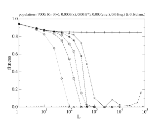
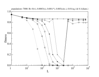
Figure 3: As Fig.2 but for oblique case: The child also learns from a teacher. The bottom part shows the fitness on a logarithmic scale for $R=0.001$ only.

Figure 4: As Fig.2a for the variants of our appendix

S. Cebrat, D. Stauffer, J.S. Sá Martins, S. Moss de Oliveira and P.M.C. de Oliveira, e-print arXiv:0911.0589 at arXiv.org (quantitative biology) (2009).

A. Gibbons, Science 329, 740-742 (2010).

J.R. Peck, G. Barreau and C.C. Heath, Genetics 145, 1171-1179 (1997).

A. Powell, S. Shennan, and M. G. Thomas, Science 324, 1298-1301 (2009)

S. Shennan, Cambridge Arch. J; 11, 5-16 (2001).