Cosmography: Supernovae Union2, Baryon Acoustic Oscillation, Observational Hubble Data and Gamma Ray Bursts

Abstract

In this paper, a parametrization describing the kinematical state of the universe via cosmographic approach is considered, where the minimum input is the assumption of the cosmological principle, i.e. the Friedmann-Robertson-Walker metric. A distinguished feature is that the result does not depend on any gravity theory and dark energy models. As a result, a series of cosmographic parameters (deceleration parameter $q_{0}$, jerk parameter $j_{0}$ and snap parameter $s_{0}$) are constrained from the cosmic observations which include type Ia supernovae (SN) Union2, the Baryon Acoustic Oscillation (BAO), the observational Hubble data (OHD), the high redshift Gamma ray bursts (GRBs). By using Markov Chain Monte Carlo (MCMC) method, we find the best fit values of cosmographic parameters in $1\sigma$ regions: $H_{0}=74.299^{+4.932}_{-4.287}$, $q_{0}=-0.386^{+0.655}_{-0.618}$, $j_{0}=-4.925^{+6.658}_{-7.297}$ and $s_{0}=-26.404^{+20.964}_{-9.097}$ which are improved remarkably. The values of $q_{0}$ and $j_{0}$ are consistent with flat $\Lambda$CDM model in $1\sigma$ region. But the value of $s_{0}$ of flat $\Lambda$CDM model will go beyond the $1\sigma$ region.

TP-DUT/2011-01

I Introduction

The kinematical approach to describe the status of universe is interesting for its distinguished feature that it does not rely on any dynamical gravity theory and dark energy models. Then it becomes crucial for its potential ability to distinguish cosmological models when a flood of dark energy models and modified gravity theories are proposed to explain the current accelerated expansion of our universe. This late time accelerated expansion of our universe was firstly revealed by two teams’ observation of type Ia supernovae ref:Riess98 ; ref:Perlmuter99 . In general, via the Taylor expansion of the scale factor $a(t)$ in terms of cosmic time $t$, the dimensionless coefficients $q_{0}$, $j_{0}$ and $s_{0}$ named deceleration, jerk and snap parameters are defined respectively, for the detailed forms please see Eq. (8, 9, 10) in the following. For convenience, they are dubbed as cosmographic parameters. These cosmographic parameters, which current values can be determined by cosmic observations, describe the kinematical status of our universe. For example, the present value of Hubble parameter $H_{0}$ describes the present expansion rate of our universe, and a negative value of $q_{0}$ means that our universe is undergoing an accelerated expansion. This kind of approach is also called cosmography ref:cosmography ; ref:ST2006 , cosmokinetics ref:cosmokinetics ; ref:cosmopara , or Friedmannless cosmology ref:Friedmannless1 ; ref:Friedmannless2 . Recently, this approach was considered by using SN in Ref. ref:kinematic2 , SN+GRBs in Ref. ref:highcosmography and SN+OHD+BAO in ref:kinematicXu , where the current status of our universe can be read. On the other hand, for a concrete dark energy model or gravity theory, when the Friedmann equation is arrived the corresponding cosmographic parameters can be derived by simple calculation. As a consequence, the corresponding parameter spaces can be fixed from cosmographic parameters space without implementing annoying data fitting procedure. However, the reliability of the cosmographic approach depends crucially on how the cosmographic parameter space is shrunk, in other words, the improvement of the figure of merit (FoM). That is the main motivation of this paper. In general, when more cosmic observational data sets are added to constrain model parameter space, the more degeneracies between model parameters will be broken. Also the FoM will be improved. So, to investigate the current status of our universe and to improve the FoM, the cosmographic parameters will be determined by more cosmic observations. When the SN and GRBs are used as distance indicators, the Hubble parameter $H_{0}$ and the absolute magnitudes of SN and GRBs are treated as notorious parameters and marginalized. That is to say, SN and GRBs can not fix the current value of Hubble parameter $H_{0}$. That is what the authors have done in Ref. ref:kinematic2 ; ref:highcosmography where the cosmographic parameters $q_{0}$, $j_{0}$ and $s_{0}$ were investigated. However, the cosmographic parameters permeate in a relative larger space. Of course, to describe the kinematical status of our universe well, one has to shrink the parameter space efficiently. Fortunately, when the Hubble parameter $H_{0}$ is fixed as done in Ref. ref:kinematicXu , the parameter space is pinned down effectively. When the snap parameter $s_{0}$ is included, high redshift observations should be added. So, in this paper we are going to use SN, BAO, GRBs, OHD to investigate the cosmographic approach. When SN data sets are used, the systematic errors are included. The BAO are detected in the clustering of the combined 2dFGRS and SDSS main galaxy samples, so it is helpful to break the degeneracies between parameters. The OHD data sets are used to fix the Hubble parameter $H_{0}$. Higher redshift data ponits are from GRBs where the correlation parameters are calibrated via cosmographic approach synchronously. For the detailed description of these data sets, please see the Appendix A.

This paper is structured as follows. In Section II, the definition of cosmographic parameters and basic expansions with respect to redshift $z$ are presented, where to consider the convergence issue, the map from $z\in(0,\infty)$ to $y=z/(1+z)\in(0,1)$ is adopted. To the expansion truncation problem, we compare the expansions with $\Lambda$CDM model in the range of redshift involved in this paper. The relative departure of Hubble parameter from that of $\Lambda$CDM model is up to $20\%$ at the redshift $z\sim 1.75$. The dfference of distance modulus between the expansion of luminosity distance and that of $\Lambda$CDM model is less than $1.6$. Section III are the main results of this paper. To obtain these results, the cosmic observational data sets from SN Ia, BAO, OHD and GRBs and MCMC method are used. The detailed descriptions are shown in the Appendix A. The main points of this paper are listed as follows: 1). BAO and OHD are used to shrink the model parameter space . 2). The calibration of GRBs and constraint to cosmographic parameters are carried out synchronously. In this way the so-called circular problem is removed. We summarize the results in Tab. 1 and Fig. 2 and Fig. 3. Section IV is a brief conclusion.

II Cosmographic Parameters

The minimum input of the cosmographic approach is the assumption of the cosmological principle, i.e. the Friedmann-Robertson-Walker (FRW) metric

$$ds^{2}=-dt^{2}+a^{2}(t)\left[\frac{dr^{2}}{1-kr^{2}}+r^{2}(d{\theta}^{2}+\sin^{2}{\theta}d{\phi}^{2})\right],$$ (1)

where the parameter $k=1,0,-1$ denotes spatial curvature for closed, flat and open geometries respectively. In this paper, we only consider the spatially flat case $k=0$.

The Hubble parameter $H(z)$ can be expanded as

$$H(z)=H_{0}+\left.\frac{dH}{dz}\right|_{0}z+\frac{1}{2}\left.\frac{d^{2}H}{dz^{2}}\right|_{0}z^{2}+\frac{1}{3!}\left.\frac{d^{3}H}{dz^{3}}\right|_{0}z^{3}+...,$$ (2)

where the subscript ’$0$’ denotes the value at the present epoch and $z=1/a(t)-1$. Via the relation

$$\frac{dt}{dz}=-\frac{1}{(1+z)H(z)},$$ (3)

one has

$$\left.\frac{dH}{dz}\right|_{0} = -\left.\frac{\dot{H}}{(1+z)H}\right|_{0}=(1+q_{0})H_{0},$$ (4)

$$\left.\frac{d^{2}H}{dz^{2}}\right|_{0} = \left.\frac{\ddot{H}}{(1+z)^{2}H^{2}}\right|_{0}+\left.\dot{H}\left(\frac{1}{(1+z)^{2}H}-\frac{\dot{H}}{(1+z)^{2}H^{3}}\right)\right|_{0}$$ (5)

$$= (j_{0}+3q_{0}+2)H_{0}-(q_{0}^{2}+3q_{0}+2)H_{0}$$

$$= (j_{0}-q_{0}^{2})H_{0},$$

$$\left.\frac{d^{3}H}{dz^{3}}\right|_{0} = -\left.\frac{H^{(3)}}{(1+z)^{3}H^{3}}\right|_{0}-\left.3\frac{\ddot{H}}{(1+z)^{2}H^{2}}\left(\frac{1}{1+z}+\frac{1}{H}\frac{dH}{dz}\right)\right|_{0}$$ (6)

$$+ \left.\frac{\dot{H}}{(1+z)H}\left[-\frac{2}{(1+z)^{2}}-\frac{2}{(1+z)H}\frac{dH}{dz}-\frac{2}{H^{2}}(\frac{dH}{dz})^{2}+\frac{1}{H}\frac{d^{2}H}{dz^{2}}\right]\right|_{0}$$

$$= (6+12q_{0}+3q_{0}^{2}+4j_{0}-s_{0})H_{0}-3(2+3q_{0}+j_{0})(2+q_{0})H_{0}$$

$$+ (1+q_{0})\left[2+2(1+q_{0})+2(1+q_{0})^{2}+q_{0}^{2}-j_{0}\right]H_{0}$$

$$= [3q_{0}^{3}+3q_{0}^{2}-j_{0}(3+4q_{0})-s_{0}]H_{0},$$

where the cosmographic parameters are defined as follows

$$H_{0} \equiv \left.\frac{da(t)}{dt}\frac{1}{a(t)}\right|_{0}\equiv\left.\frac{\dot{a}(t)}{a(t)}\right|_{0},$$ (7)

$$q_{0} \equiv -\left.\frac{1}{H^{2}}\frac{d^{2}a(t)}{dt^{2}}\frac{1}{a(t)}\right|_{0}\equiv-\left.\frac{1}{H^{2}}\frac{\ddot{a}(t)}{a(t)}\right|_{0},$$ (8)

$$j_{0} \equiv \left.\frac{1}{H^{3}}\frac{d^{3}a(t)}{dt^{3}}\frac{1}{a(t)}\right|_{0}\equiv\left.\frac{1}{H^{3}}\frac{a^{(3)}(t)}{a(t)}\right|_{0},$$ (9)

$$s_{0} \equiv \left.\frac{1}{H^{4}}\frac{d^{4}a(t)}{dt^{4}}\frac{1}{a(t)}\right|_{0}\equiv\left.\frac{1}{H^{4}}\frac{a^{(4)}(t)}{a(t)}\right|_{0}.$$ (10)

Then the Hubble parameter can be rewritten in terms of the cosmographic parameters as

$$H(z)=H_{0}\left\{1+(1+q_{0})z+(j_{0}-q_{0}^{2})z^{2}/2+[3q_{0}^{3}+3q_{0}^{2}-j_{0}(3+4q_{0})-s_{0}]z^{3}/6+...\right\}.$$ (12)

For a spatially flat FRW universe, the luminosity distance can also be expanded in terms of redshift $z$ with the cosmographic parameters

$$d_{L}(z) = cH_{0}^{-1}\left\{z+(1-q_{0})z^{2}/2-\left(1-q_{0}-3q_{0}^{2}+j_{0}\right)z^{3}/6\right.$$ (13)

$$+ \left.\left[2-2q_{0}-15q_{0}^{2}-15q_{0}^{3}+5j_{0}+10q_{0}j_{0}+s_{0}\right]z^{4}/24+...\right\}.$$

Via the relation $d_{A}(z)=d_{L}(z)/(1+z)^{2}$, one has the expansion of $d_{A}(z)$

$$d_{A}(z) = cH_{0}^{-1}\left\{z-(3+q_{0})z^{2}/2+(11-j_{0}+7q_{0}+3q_{0}^{2})z^{3}/6\right.$$ (14)

$$+ \left.(-50+13j_{0}-46q_{0}+10j_{0}q_{0}-39q_{0}^{2}-15q_{0}^{3}+s_{0})z^{4}/24+...\right\}.$$

To avoid problems with the convergence of the series for the highest redshift objects, these relations are recast in terms of the new variable $y=z/(1+z)$ ref:ztoy ; ref:ztoy2

$$H(y) = H_{0}\left\{1+(1+q_{0})y+(1+q_{0}+j_{0}/2-q_{0}^{2}/2)y^{2}+\left(6+3j_{0}+6q_{0}-4q_{0}j_{0}-3q_{0}^{2}+3q_{0}^{3}-s_{0}\right)y^{3}/6\right.$$ (15)

$$+ \left.\left(1+q_{0}-2j_{0}q_{0}+3q_{0}^{3}/2-s_{0}/2\right)y^{4}+\mathcal{O}(y^{5})\right\}$$

$$d_{L}(y) = cH_{0}^{-1}\left\{y+(3-q_{0})y^{2}/2+(11-j_{0}-5q_{0}+3q_{0}^{2})y^{3}/6\right.$$ (16)

$$+ \left.\left(50-7j_{0}-26q_{0}+10q_{0}j_{0}+21q_{0}^{2}-15q_{0}^{3}+s_{0}\right)y^{4}/24+\mathcal{O}(y^{5})\right\}$$

$$d_{A}(y) = cH_{0}^{-1}\left\{y-(1+q_{0})y^{2}/2-(1+j_{0}-q_{0}-3q_{0}^{2})y^{3}/6\right.$$ (17)

$$+ \left.(-2+j_{0}+2q_{0}+10j_{0}q_{0}-3q_{0}^{2}-15q_{0}^{3}+s_{0})y^{4}/24+\mathcal{O}(y^{5})\right\}$$

With this new variable, $z\in(0,\infty)$ is mapped into $y\in(0,1)$. And the right behavior for series convergence at any distance can be retrieved in principle ref:ztoy ; ref:ztoy2 . When the convergence problem is solved, one has to concern the expansion truncation issue. Of course, with higher orders expansion, more accurate approximation would be obtained. However, in this way, one has to introduce more model parameters beyond $H_{0}$, $q_{0}$, $j_{0}$ and $s_{0}$. How to keep the balance between the free model parameters (or expansion truncation) and comic observational data points is another complicated problem. That is beyond the scope of this paper. But we’d like to point out that the way out may be the so-call Bayesian evidence method. In fact, we can show the deviations of the expansions from $\Lambda$CDM model. For illustration, with fixed value of $\Omega_{m0}=0.27$, the relative departure of Hubble parameter from $\Lambda$CDM model (the left panel) and differences of distance modulus to $\Lambda$CDM model (the right panel) are shown in Fig. 1. Actually, in the redshift range ($z\in[0,1.75]$, please see Tab. 2) of the observational Hubble parameters, the relative departure of $\Lambda$CDM model is up to $\sim 20\%$ which is almost the same of order of error bars of OHD. In the right panel of Fig. 1, the difference of distance modulus between the expansion of luminosity distance and that of $\Lambda$CDM model is shown. At high redshift $y\sim 1$, the departure is larger up to $4$. In the redshift range of this paper, $z\in[0,9]$, the difference of distance modulus is less than $1.6$. So, up to the fourth oder of $y$, these expansions are safe.

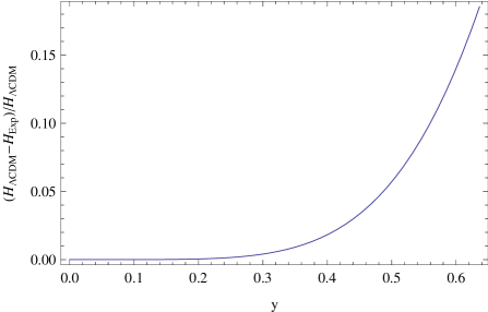
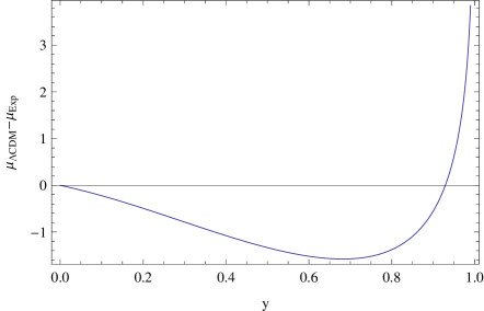
Figure 1: The Hubble parameter departure and differences of distance modulus from $\Lambda$CDM model, where $\Omega_{m0}=0.27$ is fixed.

As the reader has noticed the Taylor expansion is up to snap parameter $s_{0}$, with these cosmographic parameters the Hubble parameter is of the order $z^{3}$. However, $d_{L}(z)$ and $d_{A}(z)$ are of the order $z^{4}$. This is really from the fact that the Hubble parameter has contained one order derivative of time $t$. When it is up to the same order of $d_{L}(z)$ and $d_{A}(z)$, an extra new parameter has to be introduced. So we will classify the data sets on hand into two cases with (Case I: SN+BAO+GRBs) or without (Case II: SN+BAO+GRBs+OHD) the observational Hubble data. Another reason is that the cosmic observational data sets of SN and GRBs do not have constraint to Hubble parameter $H_{0}$. That can be seen clearly from the left panel of Fig. 2 in this paper. So, to fix the current value of Hubble parameter, the OHD data sets should be added. The reader can also see that the BAO data set is helpful to shrink the parameter space.

III Results and Discussion

In our calculations, we have taken the total likelihood function $L\propto e^{-\chi^{2}/2}$ to be the products of the separate likelihoods of SN (with systematic errors), BAO, GRBs and OHD. Then we get $\chi^{2}$

$$\chi^{2}=\chi^{2}_{SN}+\chi^{2}_{BAO}+\chi^{2}_{GRBs}+\chi^{2}_{OHD},$$ (18)

where the separate likelihoods of SN, BAO, GRBs, OHD and the current observational data sets used in this paper are shown in the Appendix A.

In our analysis, we perform a global fitting to determine the cosmographic parameters using the MCMC method. Our code is based on the publicly available CosmoMC package ref:MCMC . The results are shown in Table 1 and Figure 2.

Model		$\chi^{2}_{min}/d.o.f$		$H_{0}$		$q_{0}$		$j_{0}$		$s_{0}$		$a$		$b$
Case I		$656.821/661$		$-$		$-0.150^{+0.887}_{-0.752}$		$-5.848^{+10.0999}_{-14.412}$		$-81.268^{+91.708}_{-88.218}$		$-9.522^{+0.0909}_{-0.104}$		$1.499^{+0.173}_{-0.159}$
Case II		$670.954/676$		$74.299^{+4.932}_{-4.287}$		$-0.386^{+0.655}_{-0.618}$		$-4.925^{+6.658}_{-7.297}$		$-26.404^{+20.964}_{-9.097}$		$-9.540^{+0.104}_{-0.0999}$		$1.483^{+0.187}_{-0.166}$

Table 1: The results of $\chi^{2}_{min}$, $H_{0}$, $q_{0}$, $j_{0}$ and $s_{0}$ in Case I (SN+BAO+GRBs) and Case II (SN+BAO+GRBs+OHD), where d.o.f denotes the degree of freedom. $a$ and $b$ are parameters from Amati’s correlation of GRBs, for their definition please see Eq. 34.

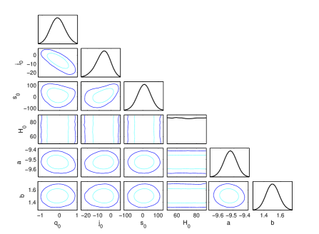
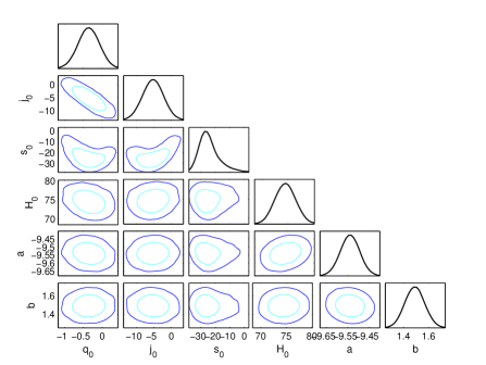
Figure 2: The 1-D marginalized distribution and 2-D contours of model parameter spaces with $1\sigma$, $2\sigma$ regions. Left Panel: Case I: SN+BAO+GRBs. Right Panel: Case II: SN+BAO+GRBs+OHD.

And the evolution curves of the Hubble parameter and distance modulus with respect to redshift $z$ are shown in Fig. 3 where the best fitted values of model parameters are adopted from the third row of Tab. 1.

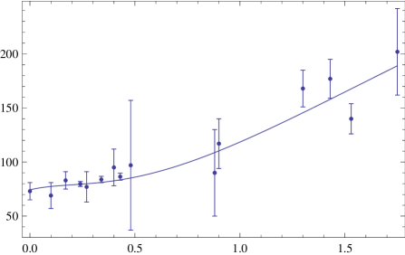
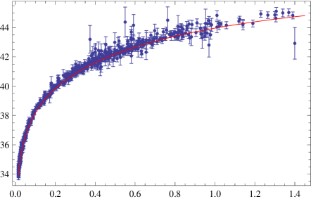
Figure 3: The Hubble parameter and distance modulus with respect to redshift $z$, where the best fitted model parameter values in the third row of Tab. 1 are adopted.

One can clearly see that when the observational Hubble data are used the $1\sigma$ error parameters space is shrunk remarkably. Put in other words, the figure of merit is improved tremendously. It is really from the fact that the Hubble parameter $H$ is expressed in terms of $z$ or $y$ with combined cosmographic parameters coefficients. Also, from the second row of Table 1, one has noticed that the BAO data set is helpful to break the degeneracy and shrink the parameter space. We can test the reliability by comparing the result with spatially flat $\Lambda$CDM model. For the spatially flat $\Lambda$CDM model, we can easily find the corresponding deceleration, jerk and snap parameters respectively

$$q_{0} = \frac{3}{2}\Omega_{m0}-1,$$ (19)

$$j_{0} = 1,$$ (20)

$$s_{0} = 1-\frac{9}{2}\Omega_{m0}.$$ (21)

When $\Omega_{m0}$ varies in the range $\Omega_{m0}\in[0,1]$, $q_{0}$ and $s_{0}$ will be in the ranges $q_{0}\in[-1,0.5]$ and $s_{0}\in[-3.5,1]$ respectively. For comparing the best fit values of cosmographic parameters in Case II with the spatially flat $\Lambda$CDM model, where the same data sets combination is used to constrain the flat $\Lambda$CDM model, one finds the corresponding result: $\Omega_{m0}=0.270_{-0.0355}^{+0.0403}$, $a=-9.398_{-0.0723}^{+0.0708}$ and $b=1.602_{-0.128}^{+0.135}$. One can clearly see that for the best fit value of $\Omega_{m0}=0.270$ in flat $\Lambda$CDM model the derived $q_{0}=-0.595$ and $j_{0}=1$ are consistent with the results obtained from cosmographic approach in $1\sigma$ region. However, the value of $s_{0}=-0.215$ of flat $\Lambda$CDM model is out the range of the $1\sigma$ region of cosmographic approach. As discussed in Ref. ref:kinematicXu , once the parameterized deceleration parameter $q(z)=q_{0}+q_{1}z/(1+z)$ ref:xupq is known, one can find the relation $q_{1}=-q_{0}-2q_{0}^{2}-j_{0}$. Also one can find other interesting relations, for example the relations between the modified gravity theory, DGP brane world model, $w=constant$, CPL parameterized equation of state of dark energy ref:ztoy2 and cosmographic parameters were investigated in Ref. ref:cosmoDai , see also in Ref. ref:kinematicXu .

IV Conclusion

In this paper, the cosmographic approach is reconsidered by using cosmic observational data which include SN Union2, BAO, GRBs and OHD via MCMC method. We find the best fit values of cosmographic parameters in $1\sigma$ ranges: $H_{0}=74.299^{+4.932}_{-4.287}$, $q_{0}=-0.386^{+0.655}_{-0.618}$, $j_{0}=-4.925^{+6.658}_{-7.297}$ and $s_{0}=-26.404^{+20.964}_{-9.097}$ which are improved remarkably. Comparing with the spatially flat $\Lambda$CDM model, one can find out that the derived values of $q_{0}$ and $j_{0}$ in flat $\Lambda$CDM are consistent with the results obtained from cosmographic approach in $1\sigma$ region. But the value of $s_{0}$ of flat $\Lambda$CDM model is out of the $1\sigma$ region of cosmographic best fit value. As investigated, the BAO data set is helpful to shrink the parameter space. When the OHD data sets are added, the parameters space is improved remarkably. The reason is from the fact that the Hubble parameter $H$ is expressed in terms of $z$ or $y$ with combined cosmographic parameters coefficients. In summary, the main points of this paper are that 1). BAO and OHD are are helpful to shrink the parameter space. 2). The calibration of GRBs and constraint to cosmographic parameters are carried out synchronously. It is away from the so-called circular problem.

Appendix A Cosmic Observational Data Sets

A.1 Type Ia Supernovae

Recently, SCP (Supernova Cosmology Project) collaboration released their Union2 dataset which consists of 557 SN Ia ref:SN557 . The distance modulus $\mu(z)$ is defined as

$$\mu_{th}(z)=5\log_{10}[\bar{d}_{L}(z)]+\mu_{0},$$ (22)

where $\bar{d}_{L}(z)$ is the Hubble-free luminosity distance $H_{0}d_{L}(z)/c=H_{0}d_{A}(z)(1+z)^{2}/c$, with $H_{0}$ the Hubble constant, and $\mu_{0}\equiv 42.38-5\log_{10}h$ through the re-normalized quantity $h$ as $H_{0}=100h~{}{\rm km~{}s}^{-1}{\rm Mpc}^{-1}$. Where $d_{L}(z)$ is defined as

$$d_{L}(z)=(1+z)r(z),\quad r(z)=\frac{c}{H_{0}\sqrt{|\Omega_{k}|}}{\rm sinn}\left[\sqrt{|\Omega_{k}|}\int^{z}_{0}\frac{dz^{\prime}}{E(z^{\prime})}\right]$$ (23)

where $E^{2}(z)=H^{2}(z)/H^{2}_{0}$. Additionally, the observed distance moduli $\mu_{obs}(z_{i})$ of SN Ia at $z_{i}$ are

$$\mu_{obs}(z_{i})=m_{obs}(z_{i})-M,$$ (24)

where $M$ is their absolute magnitudes.

For the SN Ia dataset, the best fit values of the parameters $p_{s}$ can be determined by a likelihood analysis, based on the calculation of

$$\chi^{2}(p_{s},M^{\prime}) \equiv \sum_{SN}\frac{\left\{\mu_{obs}(z_{i})-\mu_{th}(p_{s},z_{i})\right\}^{2}}{\sigma_{i}^{2}}$$ (25)

$$= \sum_{SN}\frac{\left\{5\log_{10}[\bar{d}_{L}(p_{s},z_{i})]-m_{obs}(z_{i})+M^{\prime}\right\}^{2}}{\sigma_{i}^{2}},$$

where $M^{\prime}\equiv\mu_{0}+M$ is a nuisance parameter which includes the absolute magnitude and the parameter $h$. The nuisance parameter $M^{\prime}$ can be marginalized over analytically ref:SNchi2 as

$$\bar{\chi}^{2}(p_{s})=-2\ln\int_{-\infty}^{+\infty}\exp\left[-\frac{1}{2}\chi^{2}(p_{s},M^{\prime})\right]dM^{\prime},$$

resulting to

$$\bar{\chi}^{2}=A-\frac{B^{2}}{C}+\ln\left(\frac{C}{2\pi}\right),$$ (26)

with

$$A = \sum_{i,j}^{SN}\left\{5\log_{10}[\bar{d}_{L}(p_{s},z_{i})]-m_{obs}(z_{i})\right\}\cdot{\rm Cov}^{-1}_{ij}\cdot\left\{5\log_{10}[\bar{d}_{L}(p_{s},z_{j})]-m_{obs}(z_{j})\right\},$$

$$B = \sum_{i}^{SN}{\rm Cov}^{-1}_{ij}\cdot\left\{5\log_{10}[\bar{d}_{L}(p_{s},z_{j})]-m_{obs}(z_{j})\right\},$$

$$C = \sum_{i}^{SN}{\rm Cov}^{-1}_{ii},$$ (27)

where ${\rm Cov}^{-1}_{ij}$ is the inverse of covariance matrix with or without systematic errors. One can find the details in Ref. ref:SN557 and the web site where the covariance matrix with or without systematic errors are included. Relation (25) has a minimum at the nuisance parameter value $M^{\prime}=B/C$, which contains information of the values of $h$ and $M$. Therefore, one can extract the values of $h$ and $M$ provided the knowledge of one of them. Finally, the expression

$$\chi^{2}_{SN}(p_{s},B/C)=A-(B^{2}/C),$$ (28)

which coincides to Eq. (26) up to a constant, is often used in the likelihood analysis ref:smallomega ; ref:SNchi2 . Thus in this case the results will not be affected by a flat $M^{\prime}$ distribution. It worths noting that the results will be different with or without the systematic errors. In this work, all results are obtained with systematic errors.

A.2 BAO

The BAO are detected in the clustering of the combined 2dFGRS and SDSS main galaxy samples, and measure the distance-redshift relation at $z=0.2$. BAO in the clustering of the SDSS luminous red galaxies measure the distance-redshift relation at $z=0.35$. The observed scale of the BAO calculated from these samples and from the combined sample are jointly analyzed using estimates of the correlated errors, to constrain the form of the distance measure $D_{V}(z)$ ref:Okumura2007 ; ref:Eisenstein05 ; ref:Percival

$$D_{V}(z)=\left[(1+z)^{2}D^{2}_{A}(z)\frac{cz}{H(z)}\right]^{1/3},$$ (29)

where $D_{A}(z)$ is the proper (not comoving) angular diameter distance which has the following relation with $d_{L}(z)$

$$D_{A}(z)=\frac{d_{L}(z)}{(1+z)^{2}}.$$ (30)

Matching the BAO to have the same measured scale at all redshifts then gives bao:dvratio

$$D_{V}(0.35)/D_{V}(0.2)=1.736\pm 0.065.$$ (31)

Then, the $\chi^{2}_{BAO}(p_{s})$ is given as

$$\chi^{2}_{BAO}(p_{s})=\frac{\left[D_{V}(0.35)/D_{V}(0.2)-1.736\right]^{2}}{0.065^{2}}.$$ (32)

A.3 Gamma Ray Bursts

Following ref:Schaefer , we consider the well-known Amati’s $E_{p,i}-E_{iso}$ correlation ref:Amati'srelation ; r16 ; r17 ; r18 in GRBs, where $E_{p,i}=E_{p,obs}(1+z)$ is the cosmological rest-frame spectral peak energy, and $E_{iso}$ is the isotropic energy

$$E_{iso}=4\pi d^{2}_{L}S_{bolo}/(1+z)$$ (33)

in which $d_{L}$ and $S_{bolo}$ are the luminosity distance and the bolometric fluence of the GRBs respectively. Following ref:Schaefer , we rewrite the Amati’s relation as

$$\log\frac{E_{iso}}{{\rm erg}}=a+b\log\frac{E_{p,i}}{300{\rm keV}}.$$ (34)

In ref:cosmographygrb , the correlation parameters were calibrated via cosmographic approach. Following this method, we take correlation parameters $a$ and $b$ as free parameters when GRBs is used as a cosmic constraint. We fit the Amati’s relation through the minimization $\chi^{2}$ given by ref:Schaefer

$$\chi^{2}_{GRBs}(p_{s})=\sum^{N}_{i=1}\frac{y_{i}-a-bx_{i}}{\sigma^{2}_{y,i}+b^{2}\sigma^{2}_{x,i}+\sigma^{2}_{sys}},$$ (35)

where

$$x_{i} = \log\frac{E_{p,i}}{300{\rm keV}}$$ (36)

$$y_{i} = \log\frac{E_{iso}}{{\rm erg}}=\log\frac{4\pi S_{bolo,i}}{1+z}+2\log\bar{d}_{L}$$ (37)

where $\bar{d}_{L}$ is defined as ref:wang

$$\bar{d}_{L}=H_{0}(1+z)r(z)/c,$$ (38)

and the errors are calculated by using the error propagation law ref:errors :

$$\sigma_{x,i} = \frac{\sigma_{E_{p,i}}}{\ln 10E_{p,i}}$$ (39)

$$\sigma_{y,i} = \frac{\sigma_{S_{bolo,i}}}{\ln 10S_{bolo,i}}.$$ (40)

Here $N=109$ GRBs data points are taken from ref:Wei109 . The $\chi^{2}$ is large and dominated by the systematic errors, and the statistical errors on $a$ and $b$ are small. In general the systematic error $\sigma_{sys}$ can be derived by required $\chi^{2}=\nu$ (the degrees of freedom) ref:Schaefer . Here, we take the value of $\sigma^{2}_{sys}=0.324$ from Table 1. of the case of $\Omega_{m0}=0.27$ in Ref. ref:GRBsXu . In fact, the concrete value does affect the results concluded in this paper. At last, the total error is $\sigma^{2}_{tot}=\sigma^{2}_{stat}+\sigma^{2}_{sys}$. It would be noticed that in our case, the best fit value of $a$ will be less than $2\log(c/H_{0})$ in the definition of luminosity distance $d_{L}=(1+z)r(z)$ ref:wang .

A.4 Observational Hubble Data

The observational Hubble data are based on differential ages of the galaxies ref:JL2002 . In ref:JVS2003 , Jimenez et al. obtained an independent estimate for the Hubble parameter using the method developed in ref:JL2002 , and used it to constrain the EOS of dark energy. The Hubble parameter depending on the differential ages as a function of redshift $z$ can be written in the form of

$$H(z)=-\frac{1}{1+z}\frac{dz}{dt}.$$ (41)

So, once $dz/dt$ is known, $H(z)$ is obtained directly ref:SVJ2005 . By using the differential ages of passively-evolving galaxies from the Gemini Deep Deep Survey (GDDS) ref:GDDS and archival data ref:archive1 ; ref:archive2 ; ref:archive3 ; ref:archive4 ; ref:archive5 ; ref:archive6 , Simon et al. obtained $H(z)$ in the range of $0.1\lesssim z\lesssim 1.8$ ref:SVJ2005 . In ref:0907 , Stern et al. used the new data of the differential ages of passively-evolving galaxies at $0.35<z<1$ from Keck observations, SPICES survey and VVDS survey. The twelve observational Hubble data from ref:0905 ; ref:0907 ; ref:SVJ2005 are list in Table 2. Here, we use the value of Hubble constant $H_{0}=74.2\pm 3.6{\rm km~{}s}^{-1}{\rm Mpc}^{-1}$, which is obtained by observing 240 long-period Cepheids in ref:0905 . As pointed out in ref:0905 , the systematic uncertainties have been greatly reduced by the unprecedented homogeneity in the periods and metallicity of these Cepheids. For all Cepheids, the same instrument and filters are used to reduce the systematic uncertainty related to flux calibration.

$z$	0	0.1	0.17	0.27	0.4	0.48	0.88	0.9	1.30	1.43	1.53	1.75
$H(z)\ ({\rm km~{}s^{-1}\,Mpc^{-1})}$	74.2	69	83	77	95	97	90	117	168	177	140	202
$1\sigma$ uncertainty	$\pm 3.6$	$\pm 12$	$\pm 8$	$\pm 14$	$\pm 17$	$\pm 60$	$\pm 40$	$\pm 23$	$\pm 17$	$\pm 18$	$\pm 14$	$\pm 40$

Table 2: The observational $H(z)$ data ref:0905 ; ref:0907 .

In addition, in ref:0807 , the authors took the BAO scale as a standard ruler in the radial direction, called ”Peak Method”, obtaining three more additional data: $H(z=0.24)=79.69\pm 2.32,H(z=0.34)=83.8\pm 2.96,$ and $H(z=0.43)=86.45\pm 3.27$, which are model and scale independent. Here, we just consider the statistical errors.

The best fit values of the model parameters are determined by minimizing

$$\chi_{OHD}^{2}(p_{s})=\sum_{i=1}^{15}\frac{[H_{th}(p_{s};z_{i})-H_{obs}(z_{i})]^{2}}{\sigma^{2}(z_{i})},$$ (42)

where $p_{s}$ denotes the parameters contained in the model, $H_{th}$ is the predicted value for the Hubble parameter, $H_{obs}$ is the observed value, $\sigma(z_{i})$ is the standard deviation measurement uncertainty, and the summation is over the $15$ observational Hubble data points at redshifts $z_{i}$. The OHD was firstly used to constrain cosmological model in ref:ZhangTJOHD .

References

- (1) A. G. Riess, et al., Astron. J. 116 1009(1998) [astro-ph/9805201].
- (2) S. Perlmutter, et al., Astrophys. J. 517 565(1999) [astro-ph/9812133].
- (3) M.S. Turner, A.G. Riess, Astrophys. J. 569 18(2002); M. Visser, Class. Quant. Grav. 21 2603(2004);
- (4) C. Shapiro, M. S. Turner, Astrophys. J. 649 563(2006)
- (5) R.D. Blandford, M. Amin, V. Baltz, K. Mandel, P.J. Marshall, Observing Dark Energy, 339, 27(2005) [astro-ph/0408279]
- (6) E. V. Linder, Rept. Prog. Phys. 71, 056901(2008) arXiv:0801.2968v2 [astro-ph].
- (7) Ø. Elgarøy, T. Multamäki, Mon. Not. Roy. Astron. Soc. 356 475(2005);
- (8) Ø. Elgarøy, T. Multamäki T JCAP 9 2(2006).
- (9) A.C.C. Guimaraes, J.V. Cunha and J.A.S. Lima, [arXiv:0904.3550].
- (10) V. Vitagliano, J. Q. Xia, S. Liberati, M. Viel, JCAP03(2010)005 arXiv:0911.1249v2 [astro-ph.CO].
- (11) L. Xu, W. Li, J. Lu, JCAP 0907,031(2009) arXiv:0905.4552v1 [astro-ph.CO].
- (12) C. Cattoen and M. Visser, Class. Quant. Grav. 24 (2007) 5985.
- (13) M. Chevallier, D. Polarski, Int. J. Mod. Phys. D. 10 (2001) 213; E. V. Linder, Phys. Rev. Lett. 90 (2003) 091301.
- (14) A. Lewis and S. Bridle, Phys. Rev. D 66 103511 (2002); URL: http://cosmologist.info/cosmomc/.
- (15) L. X. Xu, H. Y. Liu, Modern Physics Letters A 23 1939(2008); L. X. Xu, J. B. Lu, Modern Physics Letters A 24 369(2009). L. X. Xu, J. B. Lu and C. W Zhang, Int. J. Mod. Phys. D. 18, 1381(2009).
- (16) F. Y. Wang, Z. G. Dai, S. Qi, Astron.Astrophys.507, 53(2009) arXiv:0912.5141v2 [astro-ph.CO].
- (17) R. Amanullah et al. [Supernova Cosmology Project Collaboration], arXiv:1004.1711 [astro-ph.CO].
- (18) S. Nesseris and L. Perivolaropoulos, Phys. Rev. D 72 123519 (2005); L. Perivolaropoulos, Phys. Rev. D 71 063503 (2005); E. Di Pietro and J. F. Claeskens, Mon. Not. Roy. Astron. Soc. 341 1299 (2003); A. C. C. Guimaraes, J. V. Cunha and J. A. S. Lima, JCAP 0910 010 (2009).
- (19) E. Garcia-Berro, E. Gaztanaga, J. Isern, O. Benvenuto and L. Althaus, astro-ph/9907440; A. Riazuelo and J. Uzan, Phys. Rev. D 66 023525 (2002); V. Acquaviva and L. Verde, JCAP 0712 001 (2007).
- (20) T. Okumura, T. Matsubara, D. J. Eisenstein, I. Kayo, C. Hikage, A. S. Szalay and D. P. Schneider, ApJ 676, 889(2008) [arXiv:0711.3640]
- (21) D. J. Eisenstein, et al, Astrophys. J. 633, 560(2005) [astro-ph/0501171].
- (22) W.J. Percival, et al, Mon. Not. Roy. Astron. Soc., 381, 1053(2007) [arXiv:0705.3323]
- (23) Will J. Percival, et al, Mon.Not.Roy.Astron.Soc.401, 2148(2010), arXiv:0907.1660v3 [astro-ph.CO].
- (24) B. E. Schaefer, Astrophys. J. 660, 16 (2007) [astro-ph/0612285].
- (25) L. Amati et al., Astron. Astrophys. 390, 81 (2002) [astro-ph/0205230].
- (26) L. Amati et al., Mon. Not. Roy. Astron. Soc. 391, 577 (2008) [arXiv:0805.0377].
- (27) L. Amati, arXiv:1002.2232 [astro-ph.HE]; L. Amati, Mon. Not. Roy. Astron. Soc. 372, 233 (2006) [astro-ph/0601553].
- (28) L. Amati, F. Frontera and C. Guidorzi, arXiv:0907.0384 [astro-ph.HE].
- (29) S. Capozziello, L. Izzo, Astron. Astrophys, 490, 31( 2008); S. Capozziello, L. Izzo, arXiv:1003.5319v1 [astro-ph.CO].
- (30) Y. Wang, Phys.Rev.D 78, 123532(2008).
- (31) Herman J. Mosquera Cuesta, Habib Dumet M., Cristina Furlanetto, JCAP0807,004(2008).
- (32) H. Wei, JCAP1008, 020(2010) arXiv:1004.4951v3 [astro-ph.CO].
- (33) L. Xu, arXiv:1005.5055v1 [astro-ph.CO].
- (34) R. Jimenez and A. Loeb, Astrophys. J. 573 37 (2002) [astro-ph/0106145].
- (35) R. Jimenez, L. Verde, T. Treu and D. Stern, Astrophys. J. 593 622 (2003) [astro-ph/0302560].
- (36) J. Simon, L. Verde and R. Jimenez, Phys. Rev. D 71 123001 (2005) [astro-ph/0412269].
- (37) R. G. Abraham et al., Astron. J. 127 2455 (2004) [astro-ph/0402436].
- (38) T. Treu, M. Stiavelli, S. Casertano, P. Moller and G. Bertin, Mon. Not. Roy. Astron. Soc. 308 1037 (1999).
- (39) T. Treu, M. Stiavelli, P. Moller, S. Casertano and G. Bertin, Mon. Not. Roy. Astron. Soc. 326 221 (2001) [astro-ph/0104177].
- (40) T. Treu, M. Stiavelli, S. Casertano, P. Moller and G. Bertin, Astrophys. J. Lett. 564 L13 (2002).
- (41) J. Dunlop, J. Peacock, H. Spinrad, A. Dey, R. Jimenez, D. Stern and R. Windhorst, Nature 381 581 (1996).
- (42) H. Spinrad, A. Dey, D. Stern, J. Dunlop, J. Peacock, R. Jimenez and R. Windhorst, Astrophys. J. 484 581 (1997).
- (43) L. A. Nolan, J. S. Dunlop, R. Jimenez and A. F. Heavens, Mon. Not. Roy. Astron. Soc. 341 464 (2003) [astro-ph/0103450].
- (44) D. Stern et al., arXiv:0907.3149 [astro-ph.CO].
- (45) A. G. Riess et al., arXiv:0905.0695 [astro-ph.CO].
- (46) E. Gaztanaga et al., arXiv:0807.3551 [astro-ph.CO].
- (47) Z. Yi, T. Zhang, Mod. Phys. Lett.A 22,41(2007) [arXiv:astro-ph/0605596].