Abstract

We solve analytically the Schrödinger equation for the $N$-dimensional inverse square potential in quantum mechanics with a minimal length in terms of Heun’s functions. We apply our results to the problem of a dipole in a cosmic string background. We find that a bound state exists only if the angle between the dipole moment and the string is larger than $\pi/4$. We compare our results with recent conflicting conclusions in the literature. The minimal length may be interpreted as a radius of the cosmic string.

 

1 Introduction

We recently studied [1] the attractive inverse square potential in three dimensional quantum mechanics with a generalized uncertainty relation implying the existence of a nonzero minimal uncertainty in position measurement (minimal length) [2]. This study showed that this potential remained regular in this framework; the elementary length, plays the role of a regulator cutoff at short distances, and may be interpreted as an intrinsic dimension of the system under study.

In this paper, we generalize the aforementioned work to $N$ dimensions and arbitrary orbital momentum quantum number, and apply it to the problem of the dipole dynamics in the background of a cosmic string, where the interaction is known to be described by a two dimensional $1/R^{2}$ potential [3]. Cosmic strings are very interesting one dimensional topological defects of space-time [4]. Other types of defects are; point defects (monopoles), planar defects ( domain walls) and textures. Such defects are hypothesized to form in the phase transition of the early universe due to the process of spontaneous symmetry breaking and some of them could have survived to much later time, perhaps even to the present day [4, 5, 6].

The quantum dynamics of a point dipole in nonrelativistic quantum mechanics in a cosmic string background has been considered by several authors (see, for instance, Refs. [7, 8, 3, 9]). In Ref. [9], the author was interested in the case where the angle $\theta$ between the dipole moment and the cosmic string is such that $\theta\leq\pi/4$, in which case the potential is repulsive. The author used the method of self-adjoint extensions [10] and found that the cosmic string can bind the dipole if the potential is weakly repulsive, i.e., if one has $2M\delta/\hbar^{2}<1$, where $M$ is the particle mass and $\delta$ is the strength of the potential. The author claims that this result is an example of the classical scale symmetry breaking of the system due to a ”quantum anomaly”. Note that from a mathematical view point, a bound state may exist in a weakly repulsive $1/R^{2}$ potential because the corresponding Hamiltonian has square integrable solutions [10]. Given the counterintuitive feature of this result (i.e., the existence of a bound state in a repulsive potential), it is interesting to study the existence of bound states of that system in quantum mechanics with a minimal length and to examine whether a cosmic string keeps binding the dipole when the potential is repulsive.

The idea of modifying the standard Heisenberg uncertainty relation in such a way that it includes a minimal length has first been proposed in the context of quantum gravity and string theory [11]. It is assumed that this elementary length should be on the scale of the Planck length of $10^{-35}$m, below which the resolution of distances is impossible. The formalism based on this modified uncertainty relation, together with the concepts it implies has been discussed extensively by Kempf and his collaborators [2, 12]. Various topics were studied over the last ten years within this formalism: the hydrogen atom problem [13], the harmonic oscillator potential [14], the Casimir effect [15], the Dirac oscillator [16] and the problem of a charged particle of spin one-half moving in a constant magnetic field [17]. The modifications of the gyromagnetic moment of electrons and muons due to the minimal length have been discussed in Ref [18]. More recently several papers have been devoted to the study of the black hole thermodynamics within the minimal length formalism [19]. For a review of different approaches of theories with a minimal length scale and the relation between them, we refer the reader to Ref. [20].

For the sake of completeness, let us mention that the $1/R^{2}$ interaction that we study here in two spatial dimensions occurs in many problems of great physical interest. Indeed, this potential appears in the study of electron capture by polar molecules with static dipole moments [21, 22]. The problem of atoms interacting with a charged wire is known to provide an experimental realization of an attractive $1/R^{2}$ potential [23, 24]. The Efimov effect in three-body systems [25] arises from the existence of a long range effective $1/R^{2}$ interaction, where $R$ is built from the relative distances between the three particles. Finally, in black hole physics, the inverse square type interaction occurs naturally in the analysis of the near-horizon properties of black holes, the Bekenstein-Hawking entropy and black holes decay [26]. Note finally that the singular $1/R^{2}$ potential provides a simple example of a renormalization group limit cycle in nonrelativistic quantum mechanics  [27]. Let us mention that the condition of square integrability of the Schrödinger wave function for a singular $1/R^{2}$ potential does not lead to an orthogonal set of eigenfunctions with their corresponding eigenvalues [28, 29, 30]. This is due to the fact that the Hamiltonian operator is not essentially self-adjoint [10], so that one must define self-adjoint extensions of the Hamiltonian or equivalently require orthogonality of the wave functions [28]. The other technique used to deal with this potential is the standard regularization by a cutoff at short distances [31].

Our paper is organized as follows. In Sec. II, we study the $1/R^{2}$ potential in $N$ dimensional ($ND$) quantum mechanics with a minimal length, using the momentum representation. In Sec. III, we study the problem of a dipole in a cosmic string background. Our main result is that a bound state exists only if the angle between the dipole and the cosmic string is larger than $\pi/4$; the minimal length may be associated with the size of the cosmic string. Some concluding remarks are reported in the last section.

2 $N$ dimensional $1/R^{2}$ potential in quantum mechanics with a generalized uncertainty relation

In Ref. [1] we have solved the $s$-wave Schrödinger equation for the three dimensional $1/R^{2}$ potential in quantum mechanics when the position and momentum operators satisfy the following modified commutation relations:

$$[\widehat{X}_{i},\widehat{P}_{j}] =i\hbar[(1+\beta\widehat{P}^{2})\delta_{ij}+\beta^{{}^{\prime}}\widehat{P}_{i}\widehat{P}_{j}],\text{ \ \ }(\beta,\beta^{{}^{\prime}})>0.$$

$$[\widehat{P}_{i},\widehat{P}_{j}] =0,$$ (1)

$$[\widehat{X}_{i},\widehat{X}_{j}] =i\hbar\frac{2\beta-\beta^{{}^{\prime}}+\beta(2\beta+\beta^{{}^{\prime}})\widehat{P}^{2}}{1+\beta\widehat{P}^{2}}\left(\widehat{P}_{i}\widehat{X}_{j}-\widehat{P}_{j}\widehat{X}_{i}\right).$$

These commutators imply the generalized uncertainty relation

$$\left(\Delta X_{i}\right)\left(\Delta P_{i}\right)\geq\frac{\hbar}{2}\left(1+\beta\sum\limits_{j=1}^{N}[\left(\Delta P_{j}\right)^{2}+\left\langle\widehat{P}_{j}\right\rangle^{2}]+\beta^{{}^{\prime}}[\left(\Delta P_{i}\right)^{2}+\left\langle\widehat{P}_{i}\right\rangle^{2}]\right).$$ (2)

which leads to a lower bound of $\Delta X_{i}$, given by

$$\left(\Delta X_{i}\right)_{\min}=\hbar\sqrt{\left(N\beta+\beta^{{}^{\prime}}\right)},\text{ \ \ }\forall i.$$ (3)

Equation (2) embodies the UV/IR mixing: when $\Delta P$ is large (UV), $\Delta X$ is proportional to $\Delta P$ and, therefore, is also large (IR). This phenomenon is said to be necessary to understand the cosmological constant problem or the observable implications of short distance physics on inflationary cosmology; it has appeared in several contexts: the AdS/CFT correspondence, in noncommutative field theory and in quantum gravity in asymptotically de Sitter space [14, 33]. Another fundamental consequence of the minimal length is the loss of localization in coordinates space, so that, momentum space is more convenient in order to solve any eigenvalue problem.

In the momentum representation, the following realization satisfies the above commutation relations:

$$\widehat{X}_{i}=i\hbar\left((1+\beta p^{2})\dfrac{\partial}{\partial p_{i}}+\beta^{{}^{\prime}}p_{i}p_{j}\dfrac{\partial}{\partial p_{j}}+\gamma p_{i}\right),\text{ \ \ }\widehat{P}_{i}=p_{i}.$$ (4)

The arbitrary constant $\gamma$ does not affect the observable quantities, its choice determines the weight factor in the definition of the scalar product as follow:

$$\left\langle\varphi\left|\psi\right.\right\rangle=\int\frac{d^{N}p}{\left[1+\left(\beta+\beta^{{}^{\prime}}\right)p^{2}\right]^{1-\alpha}}\varphi^{\ast}(p)\psi(p),\text{ \ }\alpha=\frac{\gamma-\beta^{{}^{\prime}}\left(\frac{N-1}{2}\right)}{\beta+\beta^{{}^{\prime}}}.$$ (5)

In the following, we generalize the work aforementioned to arbitrary dimensions $N$ and arbitrary orbital momentum quantum number $l$.

We proceed, as in Ref. [1], by writing the Schrödinger equation, for a particle of mass $M$ in the external potential $V(R)=\delta/R^{2}$, in the form

$$(R^{2}P^{2}+2M\delta)\left.\left|\psi\right.\right\rangle=2MER^{2}\left.\left|\psi\right.\right\rangle\text{.}$$ (6)

Because of the rotational symmetry of the Hamiltonian, we can assume that the momentum space energy eigenfunctions can be factorized as [14]:

$$\psi_{N}(\vec{p})=Y_{l_{(N-1)}...l_{2}l_{1}}(\Omega)\varphi_{N}(p)\text{.}$$ (7)

Using Eq. (4) with $\gamma=0$, we obtain the following expression for $R^{2}\equiv\sum\limits_{i=1}^{N}X_{i}X_{i}$ [1, 14]:

$$R^{2} =\left(i\hbar\right)^{2}\left\{\left[1+\omega_{1}p^{2}\right]^{2}\frac{d^{2}}{dp^{2}}+\left[1+\omega_{1}p^{2}\right]\left[(N_{+}\beta+2\beta^{{}^{\prime}})p+\frac{N_{-}}{p}\right]\frac{d}{dp}\right.$$

$$\left.-\frac{L^{2}}{p^{2}}-2\beta L^{2}-\beta^{2}L^{2}p^{2}\right\},$$ (8)

where we have used the notations

$$\omega_{1}=\beta+\beta^{{}^{\prime}}\text{, \ \ \ }N_{\pm}=N\pm 1\text{, \ \ \ }L^{2}=l(l+N-2)\text{.}$$

From Eqs. (6), (7) and (8) the radial Schrödinger equation for the $\delta/R^{2}$ potential in the presence of a minimal length takes the form

$$\frac{d^{2}\varphi_{N}(p)}{dp^{2}}+\left\{\frac{4p}{p^{2}-2ME}+\frac{(N_{+}\beta+2\beta^{{}^{\prime}})p+\frac{N_{-}}{p}}{1+\omega_{1}p^{2}}\right\}\frac{d\varphi_{N}(p)}{dp}+$$

$$+\left\{2p\left[\left((N+2)\beta+3\beta^{{}^{\prime}}\right)p+\frac{N}{p}\right]+\frac{1}{1+\omega_{1}p^{2}}\left[-\beta^{2}L^{2}p^{4}+2\beta L^{2}(M\beta E-1)p^{2}\right.\right.$$

$$\left.+\left.(4M\beta E-1)L^{2}-\frac{2M\delta}{\hbar^{2}}+\frac{2MEL^{2}}{p^{2}}\right]\right\}\frac{\varphi_{N}(p)}{\left(1+\omega_{1}p^{2}\right)(p^{2}-2ME)}$$

$$=0\text{.}$$ (9)

In the case $L=0$, this equation reduces to Schrödinger equation of Ref. [1].

Introducing the dimensionless variable $z$, defined as

$$z=\frac{(\beta+\beta^{{}^{\prime}})p^{2}-1}{(\beta+\beta^{{}^{\prime}})p^{2}+1},$$ (10)

which varies from $-1$ to $+1$, and using the following notations:

$$\text{\ }\omega_{4}=\frac{\beta}{\beta+\beta^{{}^{\prime}}},\text{ \ }\omega=-M\omega_{1}E,\text{ \ }\kappa=\frac{M\delta}{2\hbar^{2}}\text{,}$$ (11)

we obtain the differential equation

$$(1-z^{2})\frac{d^{2}\varphi_{N}}{dz^{2}}+\left\{\left(\frac{N_{+}\beta+2\beta^{{}^{\prime}}}{2\omega_{1}}-\frac{3}{2}\right)(1+z)+\frac{N}{2}(1-z)+\frac{4(1+z)}{(1+2\omega)+(1-2\omega)z}\right\}\frac{d\varphi_{N}}{dz}$$

$$+\left\{\frac{1}{1-z}\left[-\left((\omega_{4}\omega+\frac{1}{4})L^{2}+\kappa\right)(1-z)^{2}-\frac{\omega_{4}^{2}L^{2}}{4}(1+z)^{2}+N_{-}(1-z)\right.\right.$$

$$\left.\left.+\frac{N_{+}\beta+2\beta^{{}^{\prime}}}{\omega_{1}}(1+z)+2\right]-\dfrac{\frac{\omega L^{2}}{2}(1-z)^{2}}{1+z}-\frac{\omega_{4}L^{2}}{2}(\omega_{4}\omega+1)(1+z)\right\}$$

$$\frac{\varphi_{N}}{(1+2\omega)+(1-2\omega)z}$$

$$=0\text{.}$$ (12)

To show that this equation can be transformed in the form of a Heun differential equation, as in the $3D$ case with $l=0$ [1], we make the following transformation:

$$\varphi_{N}(z)=(1-z)^{\lambda}(1+z)^{\lambda^{{}^{\prime}}}f(z)\text{,}$$ (13)

where $\lambda$ and $\lambda^{{}^{\prime}}$ are arbitrary constants. Then, the equation for $f(z)$ is

$$\frac{d^{2}f}{dz^{2}}+\left\{\frac{\tfrac{N_{+}\beta+2\beta^{{}^{\prime}}}{2\omega_{1}}-\tfrac{3}{2}-2\lambda}{(1-z)}+\frac{2\lambda^{{}^{\prime}}+\frac{N}{2}}{(1+z)}+\frac{4}{(1-z)\left[(1+2\omega)+(1-2\omega)z\right]}\right\}\frac{df}{dz}$$

$$+\frac{1}{(1-z^{2})^{2}\left[(1+2\omega)+(1-2\omega)z\right]}\left\{\left[(1+2\omega)+(1-2\omega)z\right]\left[\lambda(\lambda-1)(1+z)^{2}\right.\right.$$

$$-2\lambda\lambda^{\prime}(1-z^{2})+\lambda^{\prime}(\lambda^{\prime}-1)(1-z)^{2}-\lambda(\tfrac{N_{+}\beta+2\beta^{\prime}}{2\omega_{1}}-\tfrac{3}{2})(1+z)^{2}-\frac{N}{2}\lambda(1-z^{2})$$

$$\left.+\lambda^{\prime}(\tfrac{N_{+}\beta+2\beta^{\prime}}{2\omega_{1}}-\tfrac{3}{2})(1-z^{2})+\frac{N}{2}\lambda^{\prime}(1-z)^{2}\right]+(\tfrac{N_{+}\beta+2\beta^{\prime}}{\omega_{1}}-4\lambda)(1+z)^{2}$$

$$+(N_{-}+4\lambda^{\prime})(1-z^{2})-((\omega_{4}\omega+\frac{1}{4})L^{2}+\kappa)(1+z)(1-z)^{2}$$

$$\left.-\frac{\omega_{4}L^{2}}{2}(\omega_{4}\omega+1)(1+z)^{2}(1-z)-\frac{\omega_{4}^{2}L^{2}}{4}(1+z)^{3}-\frac{\omega L^{2}}{2}(1-z)^{3}+2(1+z)\right\}f$$

$$=0\text{.}$$ (14)

We choose $\lambda$ and $\lambda^{{}^{\prime}}$ by requiring that the coefficient  of $f(z)$ in Eq. (14) vanishes for $z=\pm 1$; this leads to the two equations for $\lambda$ and $\lambda^{{}^{\prime}}$ as follow:

$$\begin{array}[c]{c}\lambda^{2}-(\frac{3}{2}+\tfrac{N_{+}\beta+2\beta^{\prime}}{2\omega_{1}})\lambda+\frac{1}{2}+\tfrac{N_{+}\beta+2\beta^{\prime}}{2\omega_{1}}-\frac{\omega_{4}^{2}L^{2}}{4}=0,\\ \lambda^{{}^{\prime}2}+(\frac{N}{2}-1)\lambda^{{}^{\prime}}-\frac{L^{2}}{4}=0.\end{array}$$ (15)

The values of $\lambda$ and $\lambda^{{}^{\prime}}$ satisfying this system are

$$\begin{array}[c]{c}\lambda_{\pm}=\frac{1}{4}(3+\tfrac{N_{+}\beta+2\beta^{\prime}}{\omega_{1}}\pm\Delta_{1}),\\ \lambda_{\pm}^{\prime}=\frac{1}{2}(1-\frac{N}{2}\pm\Delta_{2}),\end{array}$$ (16)

where

$$\Delta_{1}=\sqrt{\left(\tfrac{N\beta+\beta^{\prime}}{\omega_{1}}\right)^{2}+4\omega_{4}^{2}L^{2}},\text{ \ \ \ }\Delta_{2}=\sqrt{(\frac{N}{2}-1)^{2}+L^{2}}.$$ (17)

We select the set $(\lambda,\lambda^{\prime})=(\lambda_{-},\lambda_{+}^{\prime})$; so the transformation (13) becomes

$$\varphi_{N}(z)=(1-z)^{\frac{1}{4}(3+\tfrac{N_{+}\beta+2\beta^{\prime}}{\omega_{1}}-\Delta_{1})}(1+z)^{\frac{1}{2}(1-\frac{N}{2}+\Delta_{2})}f(z).$$ (18)

By substituting $\lambda$ and $\lambda^{{}^{\prime}}$ with their values in Eq. (14), we obtain after some calculations

$$\frac{d^{2}f}{dz^{2}}+\left\{\frac{1-\frac{\Delta_{1}}{2}}{z-1}+\frac{1+\Delta_{2}}{z+1}+\frac{2}{z-z_{0}}\right\}\frac{df}{dz}+\left\{\frac{\rho z+\sigma}{(z-1)(z+1)(z-z_{0})}\right\}f=0,$$ (19)

where

$$z_{0} =\frac{2\omega+1}{2\omega-1},$$

$$\rho =\frac{10-N}{4}+\frac{N(N\beta+\beta^{\prime})}{8\omega_{1}}-\frac{3\Delta_{1}}{4}+\frac{3\Delta_{2}}{2}-\frac{\Delta_{1}\Delta_{2}}{4}$$

$$+\frac{1}{1-2\omega}\left\{\left[\frac{\omega_{4}^{2}}{2}-\omega_{4}\omega+\frac{\omega_{4}}{2}(\omega_{4}\omega+1)\right]L^{2}-\kappa\right\},$$ (20)

$$\sigma =\frac{1}{1-2\omega}\left\{\frac{1}{4}(1+2\omega)\left(\frac{N(N\beta+\beta^{\prime})}{2\omega_{1}}+2-N\right)+\frac{1}{4}(2\omega-3)\Delta_{1}\right.$$

$$\left.+\frac{1}{2}(6\omega-1)\Delta_{2}-\frac{1}{4}(1+2\omega)\Delta_{1}\Delta_{2}+\left[\frac{\omega_{4}^{2}}{2}+\omega_{4}\omega+\frac{\omega_{4}}{2}(\omega_{4}\omega+1)\right]L^{2}+\kappa\right\}\text{.}$$

Equation (19) is a linear homogeneous second-order differential equation with four singularities $z=-1,1,z_{0},\infty$, all regular. So, Eq. (19) belongs to the class of Fuchsian equations, and can be transformed into the canonical form of Heun’s equation, having regular singularities at $z=0,1,\xi_{0},\infty$ [35, 34]. The simple change of variable

$$\xi=\frac{z+1}{2}$$

leads to the following canonical form of Heun’s equation:

$$\frac{d^{2}f(\xi)}{d\xi^{2}}+\left(\frac{c}{\xi}+\frac{e}{\xi-1}+\frac{d}{\xi-\xi_{0}}\right)\frac{df(\xi)}{d\xi}+\left(\frac{ab\xi+q}{\xi(\xi-1)(\xi-\xi_{0})}\right)f(\xi)=0,$$ (21)

with the parameters

$$a =\frac{3}{2}-\frac{\Delta_{1}}{4}+\frac{\Delta_{2}}{2}-\frac{\widetilde{\nu}}{2},\text{ \ \ \ \ }$$

$$b =\frac{3}{2}-\frac{\Delta_{1}}{4}+\frac{\Delta_{2}}{2}+\frac{\widetilde{\nu}}{2},\text{ \ \ \ }c=1+\Delta_{2},\text{ \ \ \ \ }d=2,\text{ \ \ \ \ }e=1-\frac{\Delta_{1}}{2},\text{ \ \ \ }\xi_{0}=\frac{2\omega}{2\omega-1},$$

$$q =-\frac{1}{1-2\omega}\left\{1+(\frac{N}{4}-3)\omega-\frac{N(N-1)}{4}\omega_{4}\omega+\frac{\omega\Delta_{1}}{2}+(1-3\omega)\Delta_{2}+\frac{\omega\Delta_{1}\Delta_{2}}{2}-\omega_{4}\omega L^{2}-\kappa\right\},$$

$$\widetilde{\nu} =\sqrt{\left(\frac{N-1}{2}\right)^{2}(\omega_{4}-1)^{2}+\frac{1}{1-2\omega}\left\{\left[(1-2\omega)(1-2\omega_{4})-\omega_{4}^{2}(4\omega+1)\right]L^{2}+4\kappa\right\}}\text{,}$$ (22)

which are linked by the Fuchsian condition

$$a+b+1=c+d+e.$$ (23)

In the neighborhood of $\xi=0$, the two linearly independent solutions of Eq. (21) are [35]

$$f_{1}(\xi)=H(\xi_{0},q,a,b,c,d;\xi),$$ (24)

$$f_{2}(\xi)=\xi^{1-c}H(\xi_{0},q^{\prime},1+a-c,1+b-c,2-c,d;\xi),$$ (25)

where

$$q^{\prime}=q-(1-c)\left[d+\xi_{0}(1+a+b-c-d)\right].$$

$H(\xi_{0},q,a,b,c,d;\xi)$ is the Heun function defined by the series

$$H(\xi_{0},q,a,b,c,d;\xi)=1-\frac{q}{c\xi_{0}}\xi+\sum\limits_{n=2}^{\infty}C_{n}\xi^{n},$$ (26)

where the coefficients $C_{n}$ are determined by the difference equation:

$$(n+2)(n+1+c)\xi_{0}C_{n+2}=\left\{(n+1)^{2}(\xi_{0}+1)+(n+1)\left[c+d-1\right.\right.$$

$$\left.+\left.(a+b-d)\xi_{0}\right]-q\right\}C_{n+1}-(n+a)(n+b)C_{n},$$ (27)

with the initial conditions

$$C_{0}=1,\ \text{\ }C_{1}=\frac{-q}{c\xi_{0}},\text{ and }C_{n}=0,\text{ if }n<0.$$

Now, we can write the solution of the deformed Schrödinger equation (9) for the $N$ dimensional $1/R^{2}$ potential . Thus, by using Eq. (18) the solution $\psi(\xi)$, which is regular (finite) in the neighborhood of $\xi=0$, is given by

$$\varphi_{N}(\xi)=A_{N}\xi^{\frac{1}{2}(1-\frac{N}{2}+\Delta_{2})}(1-\xi)^{\frac{1}{4}\left[5+(N-1)\omega_{4}-\Delta_{1}\right]}H(\xi_{0},q,a,b,c,d;\xi),$$ (28)

where $A_{N}$ is a normalization constant.

This formula generalizes that of Ref. [1], which can be recovered in the special case: $N=3$ and $l=0$.

In the following section, we study in more detail the $2D$ case, by considering a dipole in the presence of a cosmic string.

3 Dipole dynamics in a cosmic string background

Consider a particle of mass $M$, dipole moment $D$ moving in the background field of a cosmic string. In non relativistic quantum theory the interaction between the dipole and the cosmic string is described by the potential [3, 7, 8, 9]

$$V(R)=\frac{(1-\alpha^{2})D^{2}}{48\pi\alpha^{2}R^{2}}\cos 2\theta,$$ (29)

where $\theta$ is the angle between the string and the dipole moment and $\alpha=1-4G\mu<1$ characterizes the cosmic string, with $\mu$ is the linear mass density of the string and $G$ is the gravitational constant.

The potential (29) is computed by considering the electromagnetic self-energy of the dipole due to the non-flat geometry. The space-time metric of the cosmic string background in cylindrical coordinate $(R,\phi,z)$ is [3, 7, 8, 9]

$$ds^{2}=dt^{2}-dz^{2}-dR^{2}-\alpha^{2}R^{2}d\phi^{2}\text{.}$$ (30)

Because of the cylindrical symmetry of the space, the motion of the particle along the $z$ direction is a free particle motion. By considering a cosmic string of infinite length along the $z$ direction, one only has to discuss the motion of the particle on the plane perpendicular to the $z$ direction.

The wave fuction of the dipole reads: $\psi_{2}(\vec{p})=e^{-im\phi}\varphi_{2}(p)$. The radial part, $\varphi_{2}(p)$, can be computed directly from Eq. (28) by setting $N=2$, and taking $\ 4\kappa=\frac{M(1-\alpha^{2})D^{2}}{24\pi\alpha^{2}\hbar^{2}}\cos 2\theta$. We obtain the following expression:

$$\varphi_{2}(\xi)=A\xi^{\frac{m}{2}}(1-\xi)^{\frac{1}{4}\left[5+\omega_{4}-\sqrt{(1+\omega_{4})^{2}+4\omega_{4}^{2}m^{2}}\right]}H(\xi_{0},q_{2},a_{2},b_{2},c_{2},d;\xi),$$ (31)

with the parameters

$$a_{2} =\frac{1}{4}\left(6+2m-\sqrt{(1+\omega_{4})^{2}+4\omega_{4}^{2}m^{2}}\right)-\frac{1}{2}\widetilde{\nu}_{2},\text{ \ \ \ \ }$$

$$b_{2} =\frac{1}{4}\left(6+2m-\sqrt{(1+\omega_{4})^{2}+4\omega_{4}^{2}m^{2}}\right)+\frac{1}{2}\widetilde{\nu}_{2},\text{ \ \ }$$

$$\text{\ }c_{2} =1+m,\text{ \ \ \ \ }d=2,\text{ \ \ \ \ }e_{2}=1-\frac{1}{2}\sqrt{(1+\omega_{4})^{2}+4\omega_{4}^{2}m^{2}},\text{ \ \ \ }\xi_{0}=\frac{2\omega}{2\omega-1},$$

$$q_{2} =\frac{-1}{1-2\omega}\left\{1-\frac{\omega}{2}(5+\omega_{4})+m(1-3\omega)-\omega\omega_{4}m^{2}+\frac{\omega}{2}(m+1)\sqrt{(1+\omega_{4})^{2}+4\omega_{4}^{2}m^{2}}-\kappa\right\},$$

$$\widetilde{\nu}_{2} =\sqrt{\frac{1}{4}(\omega_{4}-1)^{2}+\frac{1}{1-2\omega}\left\{4\kappa+\left[(1-2\omega)(1-2\omega_{4})-\omega_{4}^{2}(4\omega+1)\right]m^{2}\right\}}\text{.}$$ (32)

We now study the special case $m=0$ (ground state), and for convenience we take $\beta^{\prime}=0$. In this case one has $e_{2}=0$ and $q_{2}=-a_{2}b_{2}$, so Heun’s equation (21) reduces to a hypergeometric equation [1] and the wave function becomes

$$\varphi_{2}(\xi)=A(1-\xi)F(a_{2}^{\ast},b_{2}^{\ast},c_{2}^{\ast};\frac{\xi}{\xi_{0}})\text{,}$$ (33)

where

$$a_{2}^{\ast} =1-\frac{\widetilde{\nu}_{2}^{\ast}}{2}\text{, \ \ \ \ \ \ \ \ }b_{2}^{\ast}=1+\frac{\widetilde{\nu}_{2}^{\ast}}{2}\text{,}$$

$$c_{2}^{\ast} =1\text{, \ \ \ \ \ \ \ \ \ \ \ \ \ \ \ \ \ \ }\widetilde{\nu}_{2}^{\ast}=\sqrt{\frac{4\kappa}{(1-2\omega)}}\text{,}$$ (34)

$$\xi =\frac{(\beta+\beta^{{}^{\prime}})p^{2}}{(\beta+\beta^{{}^{\prime}})p^{2}+1}\text{, }\ \text{\ }\xi_{0}=\frac{2\omega}{2\omega-1}\text{.}$$

We are now ready to investigate the existence of bound states. Let us observe that, since $\cos 2\theta$ varies from $-1$ to $+1$, the parameter $\kappa$ of the dipole in the cosmic string background can be positive or negative. The author of Ref. [9] considered the repulsive case, i.e., $\theta\leq\frac{\pi}{4}$, and using the method of self-adjoint extensions [10], found that the system would have a bound state in a weakly repulsive potential ($0\leq 4\kappa\leq 1$). This bound state would be a consequence of a ”quantum anomaly” [10].

As discussed in detail in Ref. [1] for the $3D$ case, the physical eigenfunctions of the Hamiltonian must behave at large momenta as $p^{2}\varphi_{2}(p)\underset{p\rightarrow\infty}{=}0$. This boundary condition emerged naturally from the integral equation corresponding to the differential equation. It determines the physical behavior of the wave function in this asymptotic region.We get from Eq. (33) the following quantization condition:

$$F(a_{2}^{\ast},b_{2}^{\ast},c_{2}^{\ast};\frac{2\omega-1}{2\omega})=0$$ (35)

In order to examine the existence of bound states for the dipole in a cosmic string background, we have plotted the hypergeometric function in Eq. (35) as a function of $\omega=-M\beta E$ for fixed $4\kappa=$ $\frac{M(1-\alpha^{2})D^{2}}{24\pi\alpha^{2}\hbar^{2}}\cos 2\theta$. The energy eigenvalues $\omega_{n}$ are determined by the zeros of the function $F(a_{2}^{\ast},b_{2}^{\ast},c_{2}^{\ast};\frac{2\omega-1}{2\omega})$ of Eq. (35). Figure 1 shows that there are no bound states for a weakly repulsive potential. The parameters are taken identical to that used in Ref. [9], namely $\theta=\pi/12$, $D=1$, $\alpha=0.2$ for the dashed curve and $\theta=\pi/8$, $D=1.6$, $\alpha=0.2$ for the solid curve. In Ref. [9] one predicts one bound state depending on the value of the self-adjoint extensions parameter ($\sum$). In quantum mechanics with a minimal length, for any value of $\beta$ and $\beta^{\prime}$, there is no bound state in the weakly repulsive potential. Figure 2 shows that in the case $\theta=\pi/4$ (absence of interaction, i.e., $\kappa=0$) the cosmic string cannot bind the dipole. In Ref. [9], on the other hand, one bound state exists even if the strength of the potential is zero.

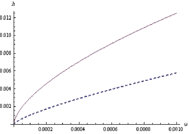
Figure 1: $h\equiv F(a_{2}^{\ast},b_{2}^{\ast},c_{2}^{\ast};\frac{2\omega-1}{2\omega})$ as a function of $\omega$, the dashed curve corresponds to $4\kappa=0.2758$ and the solid curve corresponds to $4\kappa=0.5767.$ All quantities $a_{2}^{\ast},b_{2}^{\ast},c_{2}^{\ast},$ $\omega,$ $\kappa$ are dimensionless.

Figures 3 and 4 show the appearance of bound states for $\theta>\pi/4$ (attractive potential). The energy of the ground state ($\omega_{0}$) is finite; for $\kappa=-1/20$, $\omega_{0}=5.10^{-4}$ and for $\kappa=-3/2$, $\omega_{0}=0.52$. As in Ref. [8] for ordinary quantum mechanics, there are many almost identical, excited states with $\omega\simeq 0$ (accumulation point). In Fig. 4, we can see the energy of the first excited state.

Figure 2: $h\equiv F(a_{2}^{\ast},b_{2}^{\ast},c_{2}^{\ast};\frac{2\omega-1}{2\omega})$ as a function of $\omega$, for $\kappa=0.$ All quantities $a_{2}^{\ast},b_{2}^{\ast},c_{2}^{\ast},$ $\omega,$ $\kappa$ are dimensionless.

Figure 3: $h\equiv F(a_{2}^{\ast},b_{2}^{\ast},c_{2}^{\ast};\frac{2\omega-1}{2\omega})$ as a function of $\omega$, for $4\kappa=-1/5.$ All quantities $a_{2}^{\ast},b_{2}^{\ast},c_{2}^{\ast},$ $\omega,$ $\kappa$ are dimensionless.

Figure 4: $h\equiv F(a_{2}^{\ast},b_{2}^{\ast},c_{2}^{\ast};\frac{2\omega-1}{2\omega})$ as a function of $\omega$, for $4\kappa=-6.$ All quantities $a_{2}^{\ast},b_{2}^{\ast},c_{2}^{\ast},$ $\omega,$ $\kappa$ are dimensionless.

For the sake of completeness, we consider now the case where $\theta>\frac{\pi}{4}$ ($\nu=$ $\sqrt{4\kappa}$ is now imaginary) and a sufficiently small deformation parameter $\beta$ such that $\omega=-\beta ME\ll 1$. The quantization condition (35) yields the following expression for the energy levels [1]:

$$E_{n} =\frac{-\hbar^{2}}{M(\hbar\sqrt{2\beta})^{2}}\exp\left\{\frac{2}{\nu_{2}}\left[\varphi-(n+\frac{1}{2})\pi\right]\right\},$$ (36)

$$\nu_{2} =\sqrt{-4\kappa},\text{ \ \ }\varphi=\arg\left[\frac{\Gamma(i\nu_{2})}{\Gamma(1+\frac{i\nu_{2}}{2})\Gamma(\frac{i\nu_{2}}{2})}\right]$$

as one has

$$\left|E_{n}\right|\ll\frac{1}{M\beta}\text{ \ \ \ \ \ \ \ \ \ \ \ \ \ \ \ \ \ }n=0,1,2,...\text{ .}$$

This expression is similar to what was obtained in Ref. [8], in which a cutoff $a$ is introduced by hand to regularize the interaction at short distances. In the above equation, the minimal length $(\Delta R)_{\min}=\hbar\sqrt{2\beta}$ plays the same role as $a$. The author interpreted the extra parameter $a$ as characterizing the radius of the string. We argue here that this elementary length can be associated in this problem considered with the finite size of the cosmic string.

4 Summary and conclusion

The problem of the $N$ dimensional singular inverse square potential has been solved exactly for all values of the orbital momentum quantum number in the framework of quantum mechanics with a minimal length. In the momentum representation, the wave function is a Heun function for any dimension $N$, and reduces to a hypergeometric function in some special cases. This result generalize that of Ref. [1]. As an application, we have considered a dipole in a cosmic string background. This system is described by a two-dimensional $1/R^{2}$ potential in non relativistic quantum theory, where the coupling constant depends on the angle between the string and the dipole moment ($\theta$). We have given the eigenfunctions of the Hamiltonian in the presence of a minimal length, and the corresponding bound states equation. We find that the cosmic string cannot bind the dipole for $\theta\leq\frac{\pi}{4}$. This result is in contrast with that of Ref. [9]. In the case where $\theta>\frac{\pi}{4}$ we found that there exist many bound states and the energy spectrum is bounded from below. We gave an expression for the energy levels of bound states in the limit $\beta,$ $\beta^{\prime}\ll 1$. Our results agree with what was obtained in Ref. [8], where the same problem is solved using the standard regularization technique by a cutoff ($a$) at short distances. The minimal length appears to be a natural regulator and plays the same role as $a$. We argue with the author of Ref. [8] that this elementary length should be viewed as characterizing the finite radius of the cosmic string.

Acknowledgments: D. B acknowledges the Belgian Technical Cooperation (BTC) and the Algerian ministry of Higher Education and Scientific Research (MESRS) for their financial support.The work of M. B was supported by the National Fund for Scientific Research (FNRS), Belgium.

References

• [1] D. Bouaziz and M. Bawin, Phys. Rev. A 76, 032112 (2007).
• [2] A. Kempf, G. Mangano, and R. B. Mann, Phys. Rev. D 52, 1108 (1995).
• [3] Y. Grats and A. García, Class. Qantum. Grav. 13, 189 (1996).
• [4] A.-C. Davis and T. W. B. Kibble, Contemp. Phys. 46, 313 (2005).
• [5] T. W. B. Kibble, J. Phys. A: Math. Gen. Vol. 9, N. 8, 1387 (1976); T. W. B. Kibble, Phys. Rev. D, 26, N. 2, 435 (1982).
• [6] A. Vilenkin and E. P. S. Shellard, Cosmic Strings and Other Topological Defects. Cambridge University Press, Cambridge, U. K., 1994).
• [7] C. A. de Lima Ribeiro, C. Furtado,  V. B. Bezera and F. Moraes J. Phys. A: Math. Gen. 34, 6119 (2001).
• [8] C. A. de Lima Ribeiro, C. Furtado, and F. Moraes, Mod. Phys. Lett. A 20, 1991 (2005).
• [9] P. R. Giri, Phys. Rev. A 76, 012114 (2007).
• [10] K. Meetz, Nuovo Cimento 34, 690 (1964).
• [11] D. Amati, M. Ciafaloni, and G. Veneziano, Phys. Lett. B 216, 41 (1989); M. Magiore, Phys. Lett. B 319, 83 (1993); L. J. Garay, Int. J. Mod. Phys. A 10, 145 (1995).
• [12] A. Kempf, J. Math. Phys. 35, 4483 (1994); H. Hinrichsen and A. Kempf, J. Math. Phys. 37, 2121 (1996); A. Kempf, J. Phys. A: Math. Gen. 30, 2093 (1997); A. Kempf, J. Math. Phys. 38, 1347 (1997); A. Kempf and G. Mangano, Phys. Rev. D 55 , 7909 (1997).
• [13] F. Brau, J. Phys. A: Math. Gen. 32, 7691 (1999); R. Akhoury and Y.-P. Yao, Phys. Lett. B 572, 37 (2003); S. Benczik, L. N. Chang, D. Minic, and T. Takeuchi, Phys. Rev. A 72, 012104 (2005); M. M. Stetsko and V. M. Tkachuk, Phys. Rev. A 74, 012101 (2006); M. M. Stetsko, Phys. Rev. A 74, 062105 (2006).
• [14] L. N. Chang, D. Minic, N. Okamura, and T. Takeuchi, Phys. Rev. D 65, 125027(2002)
• [15] Kh. Nouicer, J. Phys. A: Math. Gen. 38, 10027 (2005); U. Harbach and S. Hossenfelder, Phys. Lett. B 632, 379 (2006).
• [16] Kh. Nouicer, J. Phys. A: Math. Gen. 39, 5125 (2006); C. Quesne and V. M. Tkachuk, J. Phys. A : Math. Gen. 38, 1747 (2005).
• [17] Kh. Nouicer, J. Math. Phys. 47, 122102 (2006).
• [18] U. Harbach, S. Hossenfelder, M. Bleicher and H. Stoecker, Proceedings of the Nuclear Physics Winter Meeting 2004, Bormio, Italy; e-print arXiv:hep-ph/0404205.
• [19] K. Nouicer, Phys. Lett. B 646, 63 (2007) ; Y-W. Kim and Y-J Park, Phys. Lett. B V. 655, Issue. 3-4, 172 (2007); K. Nouicer, Class. Quantum. Grav.25, 075010 (2008); Y-W. Kim and Y-J Park, Phys. Rev. D 77, 067501 (2008).
• [20] S. Hossenfelder, Class. Quant. Grav. 23, 1815 (2006).
• [21] M. Bawin, Phys. Rev. A 70, 022505 (2004).
• [22] M. Bawin, S. A. Coon and B. R. Holstein, Int. Jour. Mod. Phys A, Vol. 22, N. 27, 4901 (2007), and references therein.
• [23] J. Denschlag, G. Umshaus and J. Schmiedmayer, Phys. Rev. Lett, 81, 737 (1998).
• [24] M. Bawin and S. Coon, Phys. Rev. A 63, 034701 (2001).
• [25] V. Efimov, Sov. J. Nucl. Phys. 12. 589 (1971).
• [26] T. R. Govindarajan, V. Suneeta and S. Vaidya, Nucl. Phys. B 583, 291 (2000); D. Birmingham, K. S. Gupta and S. Sen, Phys. Lett. B. 505, 191 (2001); K. S. Gupta and S. Sen, Phys. Lett. B. 526, 121 (2002); K. S. Gupta and S. Sen, Phys. Lett. B. 574, 93 (2003); K. S. Gupta, Int. Jour. Mod. Phys A, Vol. 20, N. 11, 2485 (2005).
• [27] S. R. Beane, P. F. Bedaque et al, Phys. Rev. A 64, 042103 (2001); M. Bawin and S. Coon, Phys. Rev. A 67, 042712 (2003); E. Braaten and D. Phillips, Phys. Rev. A 70, 052111 (2004).
• [28] K. M. Case, Phys. Rev. 80, 797 (1950).
• [29] A. M. Perelemov and V. S. Popov, Teor. Mat. Fiz. 4, 48 (1970) [Theor. Math. Phys. 4, 664 (1970)].
• [30] G. H. Shortey, Phys. Rev, 38, 120 (1931); F. L. Scarf, Phys. Rev, 109, 2170 (1958); W. M. Frank, D. J. Land and R. M. Spector, Rev. Mod. Phys. 43, 36 (1971); L. Landau and E. M. Lifshitz, Quantum Mechanics, Vol. 3 (Pergamon Press, London, 1958) p. 118; P. M. Morse and H. Feshbach, Methods of Theoretical Physics, Part II (McGraw-Hill, New York, 1953), pp. 1665-1667.
• [31] K. S. Gupta and S. G. Rajeev, Phys. Rev. D 48, 5940 (1993); H. E. Camblong, L. N. Epele, H. Fanchiotti, and C. A. Garcí, Phys. Rev. Lett. 85, 1590 (2000); S. A. Coon and B. R. Holstein, Am. J. Phys. 70, 513 (2002); H.-W. Hammer and B. G. Swingle, Anal. Phys, 321, 306 (2006).
• [32] Milton Abramowitz and Irene A. Stegum, Handbook of Mathematical Functions With Formulas, Graphs, and Mathematical Tables; Fifth Printing (U. S. Government Printing Office, Washington D. C., 1966), pp. 556-565.
• [33] S. Benczik et al, Phys. Rev. D 66, 026003 (2002), and references therein.
• [34] A. Ronveaux, Heun’s Differential Equations. Oxford, England : Oxford University Press (1995).
• [35] C. Snow, Hypergeometric and Legendre Functions With Applications to Integral Equations of Potential Theory, National Bureau of Standards Applied Mathematics Series (U. S. Government Printing Office, Washington D. C. 1952), Vol. 19, pp. 87-101.