Dependence of direct detection signals on the WIMP velocity distribution
Abstract:
The signals expected in WIMP direct detection experiments depend on the ultra-local dark matter distribution. Observations probe the local density, circular speed and escape speed, while simulations find velocity distributions that deviate significantly from the standard Maxwellian distribution. We calculate the energy, time and direction dependence of the event rate for a range of velocity distributions motivated by recent observations and simulations, and also investigate the uncertainty in the determination of WIMP parameters. The dominant uncertainties are the systematic error in the local circular speed and whether or not the MW has a high density dark disc. In both cases there are substantial changes in the mean differential event rate and the annual modulation signal, and hence exclusion limits and determinations of the WIMP mass. The uncertainty in the shape of the halo velocity distribution is less important, however it leads to a systematic error in the WIMP mass. The detailed direction dependence of the event rate is sensitive to the velocity distribution. However the numbers of events required to detect anisotropy and confirm the median recoil direction do not change substantially.
1 Introduction
Weakly Interacting Massive Particles (WIMPs) are a well motivated dark matter candidate [1, 2, 3]. They can be directly detected in the lab via their elastic scattering off target nuclei in dedicated detectors [4] and experiments are now probing the theoretically favoured regions of parameter space [5, 6, 7].
The nuclear recoil event rate is energy, time and direction dependent. Due to the Earth’s orbit about the Sun the net velocity of the lab with respect to the Galactic rest frame varies over the course of a year. The net speed is largest in the Summer and hence there are more high speed WIMPs, and less low speed WIMPs, in the lab frame. This produces an energy dependent annual modulation in the event rate with amplitude of order a few per-cent [8]. The WIMP flux in the lab frame is sharply peaked in the direction of motion of the Sun (towards the constellation CYGNUS), and hence the recoil spectrum is peaked in the direction opposite to this [9]. This directional signal is far larger than the annual modulation; the event rate in the backward direction is roughly an order of magnitude larger than that in the forward direction [9]. A detector which can measure the recoil directions is required to detect this signal (see Ref. [10] for an overview of the status of directional detection experiments). The time and direction dependence of the event rate are signals which can be used to discriminate WIMP induced recoils from backgrounds, while the energy dependence of the event rate can be used to measure the WIMP mass [11, 12, 13, 14, 15, 16].
The energy [17, 18], time [19, 20, 21, 22, 23, 24, 25, 26] and direction [27, 28, 29] dependence of the event rate all depend on the ultra-local WIMP distribution. Historically analytic halo models have been used to calculate the WIMP signals and analyse data. In the past few years velocity distributions from high resolution simulations of the formation of Milky Way like halos [30, 31, 32, 33, 34, 35] have been used to calculate some of the WIMP signals [36, 37, 38, 32, 39, 34, 35, 40, 41].
In this paper we study the energy, time and direction dependence of the elastic scattering event rate for a range of velocity distributions motivated by recent observations and simulations. Where possible we use WIMP and target nuclei independent parameterisations of the event rate. We also investigate the uncertainty in exclusion limits, determinations of the WIMP mass and the number of events required to detect the directional signal. For studies of the impact of uncertainties in the WIMP velocity distribution on the interpretation of data from recent experiments see Refs. [38, 34, 35, 40, 41, 42] for elastic scattering, Refs. [39, 34, 35, 41] for inelastic scattering and Ref. [41] for momentum dependent scattering.
In Sec. 2 we review the calculation of the event rate. In Sec. 3 we discuss recent results, in particular from numerical simulations, on the local dark matter distribution and present the velocity distributions which we will use to calculate the WIMP signals in Sec. 4. Finally we conclude with a summary in Sec. 5.
2 Event rate
Assuming spin-independent coupling the differential event rate (number of events per unit energy, per unit time, per unit detector mass) is given by [1, 11]
| (1) |
where is the ultra-local WIMP density, the normalised ultra-local WIMP speed distribution in the rest frame of the detector, the WIMP scattering cross section on the proton, the WIMP-proton reduced mass, and the mass number and form factor of the target nuclei respectively and is the recoil energy. The lower limit of the integral, , is the minimum WIMP speed that can cause a recoil of energy :
| (2) |
where is the atomic mass of the detector nuclei and the WIMP-nucleon reduced mass.
The WIMP speed distribution in the detector rest frame is calculated by carrying out, a time dependent, Galilean transformation: 111Formally the effects of gravitational focusing by the Sun should be taken into account [43, 44], however the resulting modulation in the differential event rate is small and only detectable with a very large number of events [43].. The Earth’s motion relative to the Galactic rest frame, , is made up of three components: the motion of the Local Standard of Rest (LSR), , the Sun’s peculiar motion with respect to the LSR, , and the Earth’s orbit about the Sun, . We use , where is the local circular speed, and [45] in Galactic co-ordinates (where points towards the Galactic center, is the direction of Galactic rotation and towards the North Galactic Pole) and the expressions for the Earth’s orbit from Ref. [46].
The differential event rate, eq. (1), depends on the target nuclei mass and also the (a priori unknown) WIMP mass. It is therefore useful (c.f. Ref. [17]) to consider the ‘WIMP and target independent’ quantity
| (3) |
The prefactor here is chosen to make dimensionless (and of order unity) while allowing variations in the local circular speed (see Sec. 3.1.2). The differential event rate can then be written as
| (4) |
where the prefactor
| (5) |
contains the WIMP and target dependent terms and is independent of the astrophysical WIMP distribution.
The direction dependence [9] of the event rate is most compactly written in terms of the radon transform of the WIMP velocity distribution [47]
| (6) |
where , is the recoil direction and is the 3-dimensional Radon transform of the WIMP velocity distribution
| (7) |
Geometrically the Radon transform, , is the integral of the function on a plane orthogonal to the direction at a distance from the origin. See Ref. [28] for an alternative, but equivalent, expression.
While the directional recoil rate depends on both of the angles which specify a given direction, the strongest signal is the differential of the event rate with respect to the angle between the recoil and the direction of solar motion, , [9, 48]
| (8) |
where is the azimuthal angle. As with the non-directional differential event it is useful to consider a dimensionless ‘WIMP and target independent’ quantity
| (9) |
so that eq. (8) can be rewritten as
| (10) |
where is defined in eq. (5).
3 Dark matter distribution
The traditional benchmark model for direct detection event rate calculations is the standard halo model (an isotropic isothermal sphere with ) which has velocity distribution
| (11) |
where is the velocity dispersion.
In Sec. 3.1 we review the status of observational measurements of the local dark matter density, circular speed and escape speed, and their relevance to the event rate calculation. In Sec. 3.2 we review results on the shape of the dark matter velocity distribution from recent numerical simulations. We conclude in Sec. 3.3 with a summary of the benchmark models which we will use to calculate the direct detection signals in Sec. 4.
3.1 Observations
3.1.1 Local density
The local density appears in the normalisation of the event rate. We use the standard value, . For a given model for the MW it is possible to determine to accuracy [56, 57], however analyses which use a range of models or model independent methods find substantially larger, of order unity, uncertainties [58, 59, 60]. Furthermore observations determine the local density averaged over a spherical shell, and the DM density in the stellar disc of simulated halos is larger than the shell average [61].
Since the normalisation is proportional to the product of and , the uncertainty in translates directly into an uncertainty in constraints on, or measurements of, . As this uncertainty is the same for all experiments we do not explicitly consider it.
3.1.2 Local circular speed
The local circular speed, the speed with which stars orbit the Galactic centre at the solar radius, is related to the velocity dispersion by the Jean’s equation [49].
| (12) |
where is the radial velocity dispersion and is the anisotropy parameter. For the standard halo model the velocity dispersion is isotropic ( so that ) and independent of radius and so that .
The standard value of is [50]. A recent analysis using Galactic masers found a significantly higher value, , [51] and this has been adopted is some subsequent direct detection work [52]. It has been argued, however, that this analysis used overly restrictive models. Bovy et al. found , assuming a flat rotation curve [53], while McMillan and Binney find values ranging from to depending on the model used for the rotation curve [54].
Given the significant systematic uncertainties in determinations of , we retain as the default value, and also consider and .
3.1.3 Local escape speed
Particles with speed, in the Galactic rest frame greater than the local escape speed, where is the potential, are not gravitationally bound. The standard halo model formally extends to infinity and therefore the speed distribution has to be truncated at ‘by hand’ (see e.g. Ref. [8]). Historically the standard value for the escape speed was . A more recent analysis, using high velocity stars from the RAVE survey, finds with a median likelihood of [55].
We use as a default the median RAVE value, , and also consider the old standard value, .
3.2 Simulations
High resolution dark matter only simulations of the formation of Milky Way like dark matter halos, find speed distributions which deviate systematically from a multivariate Gaussian (the simplest anisotropic generalisation of the Maxwellian distribution) [30, 38, 32, 34]. There are more low speed particles, and the peak in the distribution is lower. The deviation is smaller in the lab frame than in the Milky Way rest frame however [34]. Kuhlen et al. [34] study the velocity distributions of the particles in the Via Lactea 2 (VL2) [63] and GHALO [64] simulations. In each case they consider the particles centered in a 1 kpc shell centered on galactocentric radius and also 100 sample spheres of radii 1 or 1.5 kpc, each centered at a point with . The shell contains a large number () particles, allowing the average velocity distribution at the solar radius to be measured with small statistical errors. The spheres contain a smaller number of particles (), and hence have larger statistical errors, but are sensitive to local variations in the velocity distribution on scales. They find that the radial, and tangential, , velocity distributions are well fit, apart from at large , by modified gaussian distributions [38]:
| (13) | |||||
| (14) |
where are normalisation factors. The velocity distributions also have stochastic features at high speeds. There are broad bumps which vary from halo to halo, but are independent of position within a given halo and are thought to reflect the formation history of the halo [32, 34]. Kuhlen et al. [34] also find narrow spikes in some locations, corresponding to tidal streams.
We use the shell and sphere median, 16th and 84th percentile fit parameters for the VL2 [63] simulation, given in Table 1 of Ref. [34]. As discussed by Kuhlen et al., the velocity dispersion and circular speed of these dark matter only simulations is lower than expected in reality; baryonic contraction will deepen the potential well and increase the circular speed. For VL2 the most likely speed is and . To allow a comparison with the standard halo model (with standard parameters) we scale the fit parameters so that the peak of the speed distribution matches that of the standard halo model. We truncate the fitted velocity distributions ‘by hand’ at the median value from RAVE, . For the time averaged differential event rate we also consider the tabulated data from the VL2 simulation from Ref. [62]. As discussed by Ref. [34] in this case the scaling results in some of the high speed features in the distribution being pushed beyond the escape speed. These features are likely to be significant for experiments which are only sensitive to the high speed tail of the speed distribution.
It should be cautioned that the scales resolved by simulations are many orders of magnitude larger than those probed by direct detection experiments. Vogelsberger and White have developed a new technique to study the ultra-local dark matter distribution [65]. They find that the ultra-local dark matter distribution consists of a huge number of streams and is essentially smooth. Schneider et al. [66] have reached similar conclusions by studying the evolution of the first, Earth mass, microhalos to form [67, 68, 69]. This suggests (see also Ref. [70]) that the ultra-local dark matter density and velocity distribution should not be drastically different (i.e. composed of a small number of streams) to those on the scales resolved by simulations. The ultra-local velocity distribution may, however, contain some fine-grained substructure [71, 72].
The simulations discussed above contain dark matter only, while baryons dominate in the inner regions of the Milky Way. Simulating baryonic physics is extremely difficult, and producing galaxies whose detailed properties match those of real galaxies is an outstanding challenge. Some recent simulations have found that late merging sub-halos are preferentially dragged towards the disc, where they are destroyed leading to the formation of a co-rotating dark disc (DD) [31, 33, 35].
The properties (density and velocity distribution) of the DD are highly uncertain. We consider 3 benchmark models, which aim to broadly span the range of plausible properties. The first benchmark model follows Ref. [37] modelling the DD velocity distribution as a gaussian with isotropic dispersion, and lag , matching (roughly) the kinematics of the Milky Way’s stellar thick disc. We use the central value of the DD density from Ref. [37], , where is the local halo density.
Ref. [73] argues that to be consistent with the observed morphological and kinematic properties of the Milky Way’s thick disc, the Milky Way’s merger history must be quiescent compared with typical CDM merger histories. Hence the DD density must be relatively small, , at the lower end of the range of values considered in Ref. [37]. Refs. [73, 40] also argue that the DD velocity dispersion is likely to be substantially larger than that of the stellar thick disc. In order to study the effects of increasing the DD velocity dispersion and decreasing the density we consider two further benchmark models, one with and and one with and . In both cases we keep and maintain the assumption of an isotropic gaussian velocity distribution. Ref. [40] argues that the DD velocity distribution is better fit by a Tsallis distribution [74]. Given the substantial uncertainties in the DD density and velocity dispersion we do not investigate the effect of the uncertainty in the shape of the dark disc velocity distribution. For all three benchmark dark disc models, for simplicity and following Ref. [37], we use the standard halo model with standard parameters for the dark matter halo and fix the total local density to the standard value .
| label | properties |
|---|---|
| SHSP | standard halo model (SH) with , |
| SHH | SH with , |
| SHL | SH with , |
| SHH | SH with , |
| SIMsh | scaled modified Maxwellian fit to VL2 shell data, eq. (13) from Ref. [34]: |
| , , , . | |
| SIMspmed | scaled median modified Maxwellian fit to VL2 sphere data: |
| , , , . | |
| SIMsp16 | scaled 16th percentiles modified Maxwellian fit to VL2 sphere data: |
| , , , . | |
| SIMsp84 | scaled 84th percentiles modified Maxwellian fit to VL2 sphere data: |
| , , , . | |
| DDHL | SHSP plus a dark disk with , , |
| DDLL | SHSP plus a dark disk with , , |
| DDLH | SHSP plus a dark disk with , , |
3.3 Summary
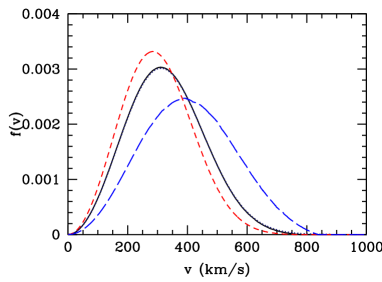
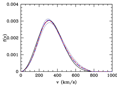
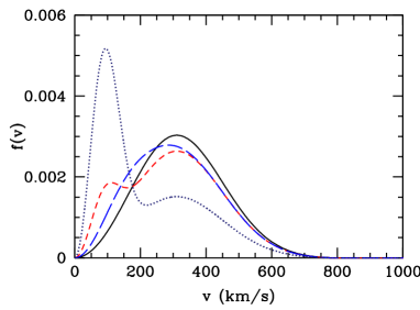
The benchmark models we consider are summarised in Table 1. For compactness we refer to the standard halo model with and as the standard halo model with standard parameters (SHSP). The normalised speed distribution for each of the models is plotted in fig. 1. For the standard halo model, increasing (decreasing) increases (decreases) both , the value of at which peaks, and also the width of . The speed distribution of a pure DD has the same qualitative shape as the standard halo model. The effect of a DD on the total normalised speed distribution depends strongly on both the DD density and speed dispersion. With a high DD density and a low DD velocity dispersion there is a large additional peak in the speed distribution as low speed. As the DD density is decreased the height of the peak decreases. If the DD velocity dispersion is increased the separation of the DD speed peak and halo speed peak decreases. For DDLH, which has a low DD density and a large speed dispersion, the speed distribution has a single peak, at a lower speed than the standard halo model. As previously found [34] the speed distributions from the modified Maxwellian fits to the VL2 simulation data have less low speed and more high speed particles than the standard halo model with the same peak speed, . However the differences, in the lab frame, are fairly small [34]. The best fit to the shell data and the median fit to the sphere data are fairly similar. The scatter between sphere fits is . If the simulation fits were compared to a standard halo with the same circular speed, (which is the observable quantity) rather than the same peak speed, , the deviations from the standard halo model would, however, be larger.
4 Results
4.1 Differential event rate
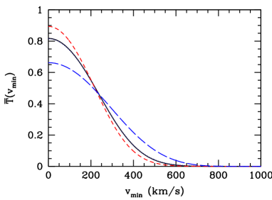
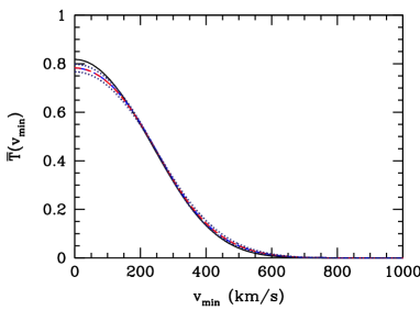
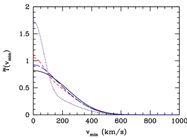
In fig. 2 we plot , the time averaged value of the model independent parameterisation of the differential event rate, eq.(3), for each of the benchmark velocity distributions. For the standard halo model is approximately given by [11]
| (15) |
where and are constants of order unity i.e. increasing decreases both the overall normalisation and the rate at which decreases with increasing . Varying the escape speed has a negligible effect, apart from at large . With a DD is larger, and the initial decrease in as is increased is more rapid. The smaller the DD density and the closer the speed dispersion to that of the standard halo, the smaller the difference from the standard halo. For the two models with a low DD density, the change in is relatively small for . Consequently in these cases there will only be a significant change in the mean differential event rate if the WIMP mass and/or experimental energy threshold are sufficiently low. For the modified Maxwellian fits to the VL2 simulation data the shape of is qualitatively similar to that of the standard halo model, but is smaller and the fall off of with increasing is slower. The shell/median sphere fit are similar and the difference between them and the standard halo is similar to the spread in the sphere fits. The differences are small, however, compared with those from the uncertainty in the value of . We have checked that using the tabulated data from the VL2 simulation from Ref. [62] produces a similar uncertainty in as the spread in the sphere fits.
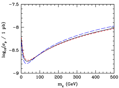
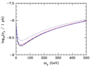
In the absence of a positive signal experiments place exclusion limits on the WIMP mass and cross-section, which depend on the WIMP distribution [75, 41]. To illustrate the effect of the uncertainty in the WIMP velocity distribution on exclusion limits we calculate exclusion limits for an ideal experiment (perfect energy resolution, perfect efficiency, zero background and zero energy threshold) using a Ge target with an exposure . For each mass we find the cross-section for which the expected number of events is equal to three (the upper confidence limit when zero events are observed) [76]. The resulting exclusion limits are shown in fig. 3 for each velocity distribution. The total WIMP flux is proportional to the mean WIMP speed, which for the standard halo model is proportional to . Therefore the naive expectation is that increasing increases the total event rate and hence leads to a tighter constraint on . As can be seen in fig. 3 this is the case for small . For larger the, energy dependent, suppression of the event rate by the form factor, means that when is increased the total event rate in fact decreases and the limit on becomes weaker (see also Ref. [52]). Increasing the energy threshold weakens the constraints, and increases the mass at which the transition occurs. Changing the escape speed only affects the exclusion limits significantly for light () WIMPs, see Ref. [41]. For a high density DD the increase in for small means that the exclusion limit is a factor of a few weaker for all . For the low density DD models and the simulation fits the change in the exclusion limit is, as expected, relatively small.
Energy dependent efficiency and/or background events will change the shape of the exclusion limits, see e.g. Ref. [75, 41]. As discussed above the uncertainty in the local density translates directly into an uncertainty in which is the same for all experiments. Note that, as pointed out in Ref. [41], the values of and are correlated.
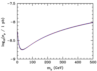
Once events are detected the shape of the energy spectrum can be used to measure the WIMP mass [11, 12, 13, 14, 15, 16]. Uncertainty in the velocity distribution leads to a systematic uncertainty in the determination of the WIMP mass [14]. We use the method used in Refs. [14, 16] to calculate the limits on the WIMP mass which would be obtained for each velocity distribution, if the data were analysed assuming the standard halo model with standard parameters. As before we assume an ideal Ge detector 222See Ref. [16] for an exploration of how varying the detector capabilities affects the WIMP mass determination. a WIMP cross-section, and an exposure of . We estimate the WIMP mass and cross-section by maximising the extended likelihood function, e.g. Ref. [77]:
| (16) |
Here is the number of events observed, are the energies of the events observed, is the normalised differential event rate and is the mean number of events. We calculate the probability distribution of the maximum likelihood estimator of the WIMP mass, for each input WIMP mass, by simulating experiments and finding the , and percentiles, , of the mass distribution.
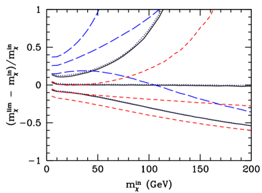
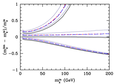
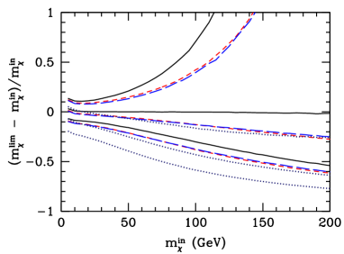
The fractional mass limits, are plotted in fig. 4 as a function of the input WIMP mass, . As discussed in Refs. [13, 14, 16], assuming an erroneous value of leads to a systematic error in the mass determination which increases with increasing :
| (17) |
A dark disc has a similar effect. There is a population of WIMPs with lower speeds than assumed, and hence the WIMP mass is systematically underestimated. The systematic underestimate is substantial (, increasing with increasing ) if the DD density is large and the speed dispersion is significantly different from that of the halo. For the two models with a low DD density, the systematic underestimate is smaller, . The larger width of the modified Maxwellian speed distribution leads to a systematic overestimate of the WIMP mass in the range , increasing weakly with increasing WIMP mass.
4.2 Annual modulation
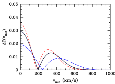
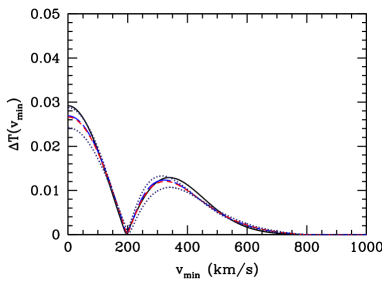
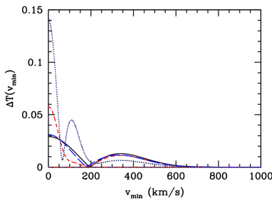
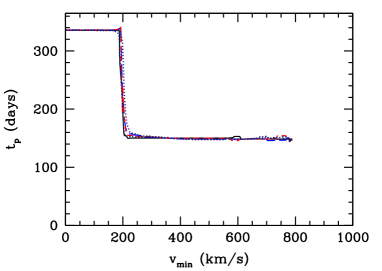
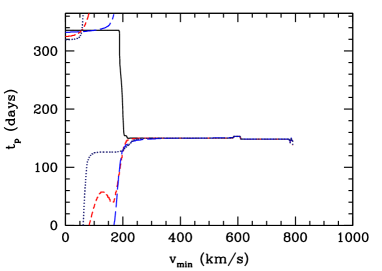
We consider the amplitude of the modulation in the model independent parameterisation of the differential event rate, , 333Some papers, e.g. Ref. [34], consider the fractional annual modulation, which is largest for large . and the date on which this maximum occurs. For small , the maximum event rate occurs in Winter [78]. As is increased, initially decreases to zero at which point the phase of the annual modulation changes rapidly and the maximum occurs in Summer. As is increased further the amplitude increases one more to a local maximum (which we refer to as the Summer maximum), before decreasing again and tending to zero [78, 79].
In figs. 5 and 6 we plot and the day of the year on which the maximum occurs, , respectively, for each of the benchmark velocity distributions. We do not include a plot of for the standard halo model as the low and high values of only change by day as is varied.
For the standard halo model, as is increased the most likely velocity and the width of the velocity distribution both increase. Consequently and the Summer maximum of both decrease, the value of at which the Summer maximum occurs increases and the decline in the amplitude for large is less rapid. The value of at which the maximum switches from Winter to Summer increases.
For a pure DD (no halo) the behaviour would be qualitatively similar to the standard halo model. Due to the speed distribution peaking at a smaller speed, and having smaller dispersion, and the Summer maximum would be larger, and the phase change would happen at smaller , . When a DD is added to the standard halo the net effect is more complicated. For DDHL there are two local Summer maxima in the amplitude, a large one at from the DD and a smaller one from the halo in the usual position, . In between the maximum occurs at days. For DDLL the DD density is not high enough to produce a second Summer maximum, however is does lead to a significant variation of for . This is because for these values of the contributions from the DD and the halo are out of phase, and partly cancel. For DDLH the change from the standard halo model is fairly small.
For the modified Maxwellian distributions the qualitative behaviour of is the same as for the standard halo model; is smaller, the Summer maximum occurs at a smaller , but its amplitude can be either smaller or larger. The changes in the amplitude of the modulation are larger than those in the mean differential event rate. However, the changes from the uncertainty in are again larger than those from the uncertainty in the shape of the speed distribution (unless there is a dark disc with small speed dispersion). The change in from Winter to Summer happens more gradually, and for large is typically a few days smaller. For both the SHSP and the modified Maxwellian fits and hence the corresponding value of is hard to calculate accurately, and not particularly physically meaningful.
4.3 Direction dependence
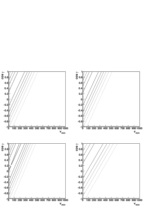


The model independent parameterisation of the direction dependence, as defined in eq. (9), is shown in figs. 7, 8 and 9 for the standard halo model, the modified Maxwellian fits to the simulation data and the dark disc models respectively. For the standard halo model [9]
| (18) |
where is the component of the Earth’s velocity parallel to the direction of Solar motion. This has a maximum value, for , of . As can be seen in fig. 7, for the standard halo model is constant for fixed . This is not the case for the other velocity distributions. For the anisotropic modified Maxwellian distribution, around the peak of the distribution as is decreased, with fixed, the value of decreases, while the contours of low fixed are convex. For the DD models the additional population of low speed WIMPs means that peaks at smaller and has a larger peak value ( for DDHL compared with for the standard halo). Around the peak of the distribution in this case as is decreased, with fixed, the value of decreases. As before, the smaller the DD density and the closer the speed dispersion to that of the standard halo, the smaller the difference from the standard halo.
We use the methods presented in Ref. [29] to calculate the number of events required to determine that the recoil distribution is not isotropic if . Briefly, we use the HADES code [80] to simulate the recoil direction distribution for a detector with energy threshold 444It is impossible for a directional detector to have zero energy threshold, even in principle, as the lengths of the nuclear recoils tend to zero in this limit, and hence their direction is unmeasurable.. We assume that the recoil directions, including their senses, are reconstructed perfectly in 3d and the background is zero. These are optimistic assumptions and therefore our results provide a lower limit on the number of events required by a real detector. For 3-d data the most powerful test for rejecting isotropy uses the average of the cosine of the angle between the direction of solar motion and the recoil direction, [29]. We calculate the probability distribution of , for a given number of events , by Monte Carlo generating experiments and find the number of events required to reject isotropy at confidence in of experiments, . For further details see Ref. [29]. For all the velocity distributions considered .
The WIMP origin of an anisotropic recoil distribution could be checked by measuring the median recoil direction [81]. For a smooth WIMP distribution the median inverse recoil direction coincides with the direction of solar motion, modulo statistical fluctuations. The median inverse direction is defined as the direction which minimises the sum of the arc-lengths between and the individual inverse recoil directions [82]. It is found by minimising
| (19) |
where is the number of events. We determine the number of events required to confirm the direction of solar motion as the median inverse recoil direction at confidence using the distribution of , the angle between the median direction and the direction of solar motion, :
| (20) |
We calculate the probability distribution of , for a given number of events , by Monte Carlo generating experiments and find the number of events required to reject the median direction being random at confidence in of experiments, . For further details see Ref. [81]. The value of , is only weakly dependent on the velocity distribution. For SHH, while for all the other velocity distributions or .
The limited variation of and show that the directional signals are robust to (plausible) uncertainties in the velocity distribution. The modified Maxwellian fits to the simulation data do not include the stochastic features found at high speeds however. These features can cause the median inverse direction of high energy recoils to deviate from the direction of solar motion [34]. As discussed in Ref. [81] the deviation will be small unless the detector is only sensitive to the high speed tail of the speed distribution (i.e. if the WIMP mass is small and/or the energy threshold is high). Studying the median direction of high energy recoils could in fact allow high speed features to be detected, hence probing the formation history of the Milky Way.
5 Summary
Direct detection event rate calculations often assume the standard halo model, with an isotropic Maxwellian velocity distribution. It is well known, however, that the energy [17, 18, 75, 36, 37, 32, 34, 35, 40, 41], time [19, 20, 21, 22, 23, 24, 25, 26, 36, 37, 38, 32, 34, 35, 40] and direction [27, 28, 29, 34] dependence of the direct detection event rate all depend on the local WIMP distribution. We have updated these studies in light of recent numerical simulations and observational measurements of the local circular speed and escape speed.
The local circular speed has a model dependent relation to the radial velocity dispersion. Recent determinations, e.g. Refs [51, 53], have relatively small statistical errors, however Ref. [54] found values ranging from to , depending on the model of the MW assumed. The most recent determination of the local escape speed [55] finds , slightly lower than the historical standard value, . Similarly for a given model for the MW it is possible to determine the local DM density, , to accuracy [56, 57], however the systematic errors are likely to be substantially larger [58, 59, 60, 61].
High resolution dark matter only simulations of the formation of Milky Way like dark matter halos, typically find speed distributions which can be fit with a modified Maxwellian distribution which is broader than the standard Maxwellian distribution [30, 38, 32, 34]. Some simulations which include baryonic physics find that late merging sub-halos are preferentially dragged towards the disc, where they are destroyed leading to the formation of a co-rotating dark disc [31, 33, 35]. The significance of a DD for direct detection experiments depends on its density and velocity distribution, which are highly uncertain [37, 73, 40].
We have considered three types of velocity distribution: standard
Maxwellian, modified Maxwellian, standard Maxwellian plus dark
disc. In each case we use a range of parameter values motivated by
recent observations and simulations (as discussed in detail in Sec. 3).
Differential event rate and exclusion limits
The systematic uncertainty in the local circular speed, , leads to a uncertainty in the differential event rate, and hence exclusion limits. A high density DD also produces significant changes in these quantities. A low density DD will only have a significant effect if the WIMP mass and/or energy threshold are sufficiently low. The dependence on the detailed shape of the velocity distribution is small.
The normalisation of the differential event rate is directly
proportional to the product of the local density and the WIMP
cross-section. Therefore the uncertainty in the measurement of the local
density propagates directly into an uncertainty on measurements of, or
constrains on, the cross-section.
Mass determination
We studied the systematic errors in
determinations of the WIMP mass which would occur if data from a
future SuperCDMS like experiment is, erroneously, analysed assuming
the standard halo model with standard parameters.
Assuming an incorrect value of leads to a systematic error in the mass
determination which increases with increasing
[13, 14, 16]. With a DD there is a
population of WIMPs with lower speeds than assumed and hence the WIMP
mass is underestimated. The size of the systematic error varies, with
increasing , from for a high density dark disc and
from for a low density dark disc. The larger width of the
modified Maxwellian distribution leads to a smaller overestimate of .
Annual modulation
The annual modulation is more sensitive to the velocity distribution than the mean differential rate. Changing the value of or a DD with small speed dispersion can change the amplitude by a factor of order unity, while the uncertainty in the shape of the halo velocity distribution changes the amplitude by .
The phase of the modulation depends only weakly on and the
shape of the halo velocity distribution. With a small speed dispersion
DD the phase at moderate energies changes by days if
the DD density is low (high).
Direction dependence
The detailed direction dependence of the event rate is sensitive to
the velocity distribution, however the directional signals are
robust. The number of events required to detect anisotropy does not
change, while the number of events required to demonstrate that the
median inverse recoil direction
coincides with the direction of solar motion varies by of order .
Even with recent improvements in the resolution of numerical simulations and observational determinations of the dark matter parameters, there are still significant uncertainties in the direct detection signals and WIMP parameter determinations. In particular the existence of a DD could have a significant effect, depending on its density and speed dispersion.
Considering a range of, data motivated, benchmark models is an improvement on simply assuming the ‘standard halo model’. However it is still not completely satisfactory. In particular it does not provide a formal analysis of errors. Several approaches to dealing with the impact of astrophysical uncertainties on direct detection data analysis have recently been proposed. Strigari and Trotta [83] have suggested using astronomical data and a model for the Milky Way mass distribution in a Monte Carlo Markov Chain analysis of direct detection data. Peter [84] has presented an approach which involves combining data sets from different direct detection experiments and jointly constraining a parametrisation of the WIMP speed distribution and the WIMP parameters (mass and cross-section). These are promising directions, however in both cases the current implementations assume an overly restrictive form for the velocity distribution (a single isotropic Maxwellian).
Acknowledgments.
AMG is supported by STFC, is grateful to Ben Morgan, Mike Kuhlen and Simon Goodwin for useful discussions and acknowledges the use of Ben Morgan’s HADES, directional detection code.References
- [1] G. Jungman, M. Kamionkowski and K. Griest, Phys. Rept. 267 (1996) 195.
- [2] G. Bertone, D. Hooper and J. Silk, Phys. Rep. Phys. Rept. 405 (2005) 279.
- [3] Particle Dark Matter, observations, models and searches, ed. G. Bertone, CUP (2010).
- [4] M. W. Goodman and E. Witten, Phys. Rev. D 31 (1985) 3059.
- [5] V. N. Lebedenko et al., Phys. Rev. D 80 (2009) 052010, \arXivid0812.1150.
- [6] Z. Ahmed et al., Science 327 (2010) 1619, \arXivid0912.3592.
- [7] E. Aprile et al., \arXivid1005.0380.
- [8] A. K. Drukier, K. Freese and D. N. Spergel, Phys. Rev. D 33 (1986) 3495.
- [9] D. N. Spergel, Phys. Rev. D 37 (1998) 1353.
- [10] S. Ahlen et al., Int. J. Mod. Phys. A 25 (2010) 1, \arXivid0911.0323.
- [11] J. D. Lewin and P. F. Smith, Astropart. Phys. 6 (1996) 87.
- [12] J. L. Bourjaily and G. L. Kane, hep-ph/0501262.
- [13] http://particleastro.brown.edu/theses/ 060421_Monte_Carlo_Simulations_Dark_Matter_Detectors_Jackson_v3.pdf; http://cosmology.berkeley.edu/inpac/CDMSCE_Jun06/Talks/200606CDMSCEmass.pdf
- [14] A. M. Green, JCAP 08 (2007) 022, hep-ph/0703217.
- [15] M. Drees and C-L. Shan, JCAP 06 (2008) 012, \arXivid0803.4477.
- [16] A. M. Green, JCAP 07 (2008) 005, \arXivid0805.1704.
- [17] M. Kamionkowski and A. Kinkhabwala, Phys. Rev. D 57 (1998) 3256, hep-ph/9710337.
- [18] F. Donato, N. Fornengo and S. Scopel, Astropart. Phys. 9 (1998) 247, hep-ph/9803295.
- [19] M. Brhlik and L. Roszkowski, Phys. Lett. B 464 (1999) 303, hep-ph/9903468.
- [20] P. Belli et. al., Phys. Rev. D 61 (2000) 023512.
- [21] J. D. Vergados, Phys. Rev. Lett. 83 (1999) 3597; Phys. Rev. D 62 (2000) 023519, astro-ph/0001190; Phys. Rev. D 63 (2001) 063511.
- [22] P. Ullio and M. Kamionkowski, J. High Energy Phys. 0103 (2001) 049, hep-ph/0006183.
- [23] N. W. Evans, C. M. Carollo and P. T. de Zeeuw, Mon. Roy. Astron. Soc. 318 (2000) 1131, astro-ph/0008156.
- [24] A. M. Green, Phys. Rev. D 63 (2001) 043005, astro-ph/0008318.
- [25] A. M. Green, Phys. Rev. D 68 (2003) 023004, astro-ph/0304446.
- [26] A. Natarajan, \arXivid1006.5716.
- [27] C. J. Copi, J. Heo and L. M. Krauss, Phys. Lett. B 461 (1999) 43, astro-ph/990449.
- [28] C. J. Copi and L. M. Krauss, Phys. Rev. D 63 (2001) 043507, astro-ph/0009467.
- [29] B. Morgan, A. M. Green and N. J. C. Spooner, Phys. Rev. D 71 (2005) 103507, astro-ph/0408047.
- [30] S. H. Hansen, B. Moore, M. Zemp and J. Stadel, JCAP 01 (2006) 014, astro-ph/0505420.
- [31] J. I. Read, G. Lake, O. Agertz and V. P. Debattista, Mon. Not. Roy. Astron. Soc. 389 (2008) 1041, \arXivid0803.2714.
- [32] M. Vogelsberger et al., Mon. Not. Roy. Astron. Soc. 395 (2009) 797, \arXivid0812.0362.
- [33] J. I. Read, L. Mayer, A. M. Brooks, F. Governato and G. Lake, Mon. Not. Roy. Astron. Soc. 397 (2009) 44, \arXivid0902.009.
- [34] M. Kuhlen et al., JCAP 02 (2010) 030, \arXivid0912.2358.
- [35] F.-S. Ling, E. Nezri, E. Athanassoula and R. Teyssier, JCAP 02 (2010) 012, \arXivid0909.2028.
- [36] J. D. Vergados, S. H. Hansen and O. Host, Phys. Rev. D 77 (2008) 023509, \arXivid0711.4895.
- [37] T. Bruch, J. Read, L. Baudis and G. Lake, Astrophys. J. 696 (2009) 920, \arXivid0804.2896.
- [38] M. Fairbairn and T. Schwetz, JCAP 01 (2009) 037, \arXivid0808.0704.
- [39] J. March-Russell, C. McCabe and M. McCullough, J. High Energy Phys. 05 (2009) 071, \arXivid0812.1931.
- [40] F.-S. Ling, Phys. Rev. D 82 (2010) 023534, \arXivid0911.2321.
- [41] C. McCabe, Phys. Rev. D 82 (2010) 023530, \arXivid1005.0579.
- [42] S. Chaudhury, P. Bhattacharjee and R. Cowsik, \arXivid1006.5588.
- [43] K. Griest Phys. Rev. D 37 (1988) 2703.
- [44] M. S. Alenazi and P. Gondolo, Phys. Rev. D 74 (2006) 083518, astro-ph/0608390.
- [45] R. Schoenrich, J. Binney and W. Dehnen, Mon. Not. Roy. Astron. Soc. 403 (2010) 1829, \arXivid0912.3693.
- [46] R. M. Green, Spherical astronomy, (1985).
- [47] P. Gondolo, Phys. Rev. D 66 (2002) 103513, astro-ph/0209110.
- [48] M. S. Alenazi and P. Gondolo, Phys. Rev. D 77 (2008) 043532, \arXivid0712.0053.
- [49] J. Binney and S. Tremaine, Galactic dynamics, Princeton University Press (2008).
- [50] F. J. Kerr and D. Lynden-Bell, Mon. Not. Roy. Astron. Soc. 221 (1986) 1023.
- [51] M. J. Reid et al., Astrophys. J. 700 (2009) 137, \arXivid0902.3913.
- [52] C. Savage, K. Freese, P.Gondolo and D. Spolyar, JCAP 09 (2009) 036, \arXivid0901.2713.
- [53] J. Bovy, D. W. Hogg and H. Rix, Astrophys. J. 704 (2009) 1704, \arXivid0907.4523.
- [54] P. J. McMillan and J. J. Binney Mon. Not. Roy. Astron. Soc. 402 (2010) 934, \arXivid0907.4685.
- [55] M. C. Smith et al., Mon. Not. Roy. Astron. Soc. 379 (2007) 755, astro-ph/0611671.
- [56] L. M. Widrow, B. Pym and J. Dubinski, Astrophys. J. 679 (2008) 1239, \arXivid0801.3414.
- [57] R. Catena and P. Ullio, JCAP 08 (2010) 004, \arXivid0907.0018.
- [58] M. Weber and W. de Boer, Astron. Astrophys. 509 (2010) 25, \arXivid0910.4272.
- [59] S. Gabari, G. Lake and J. I. Read, \arXivid1001.1038.
- [60] P. Salucci, F. Nestri, G. Gentile and C. F. Martins, \arXivid1003.3101.
- [61] M. Pato, O. Agertz, G. Bertone, B. Moore and R. Teyssier, Phys. Rev. D 82 (2010) 023531, \arXivid1006.1322.
- [62] http://astro.berkeley.edu/mqk/dmdd/
- [63] J. Diemand et al., Nature 454 (2008) 735, \arXivid0805.1244.
- [64] J. Stadel et al., Mon. Not. Roy. Astron. Soc. 398 (2009) L21, \arXivid0808.2981.
- [65] M. Vogelsberger and S. D. M. White, \arXivid1002.3162.
- [66] A. Schneider, L. M. Krauss and B. Moore, \arXivid1004.5432.
- [67] S. Hofmann, D. J. Schwarz and H. Stocker, Phys. Rev. D 64 (2001) 083507, astro-ph/0104173.
- [68] A. M. Green, S. Hofmann and D. Schwarz, Mon. Not. Roy. Astron. Soc. 353 (2004) L23, astro-ph/0309621; JCAP 08 (2005) 003, astro-ph/0503387.
- [69] J. Diemand, B. Moore and J. Stadel, Nature 433 (2005) 289, astro-ph/0501589.
- [70] M. Kamionkowski and S. M. Koushiappas, Phys. Rev. D 77 (2008) 103509, \arXivid0801.3269.
- [71] D. S. M. Fantin, M. R. Merrifield and A. M. Green, Mon. Not. Roy. Astron. Soc. 390 (2008) 1055, \arXivid0808.1050
- [72] N. Afshordi, R. Mohayee and E. Bertchinger, Phys. Rev. D 79 (2009) 083526, \arXivid0811.1582; Phys. Rev. D 82 (2010) 101301, \arXivid0911.0414.
- [73] C. W. Purcell, J. S. Bullock and M. Kaplinghat, Astrophys. J. 703 (2009) 2275, \arXivid0906.5348.
- [74] C. Tsallis, J. Stat. Phys. 52 (1988) 479.
- [75] A. M. Green, Phys. Rev. D 66 (2002) 083003, astro-ph/0207366.
- [76] C. Amsler et al. (Particle Data Group), Phys. Lett. B 667 (2008) 1.
- [77] G. Cowan, Statistical data analysis, published by Oxford University Press (1998).
- [78] J. R. Primack, D. Seckel and B. Sadoulet, Ann. Rev. Nucl. Part. Sci. 38 (1998) 751.
- [79] M. J. Lewis and K. Freese, Phys. Rev. D 70 (2004) 043501, astro-ph/0307190.
- [80] B. Morgan, Dark Matter Detection With Gas Time Projection Chambers, Ph.D. Thesis, University of Sheffield, (2004).
- [81] A. M. Green and B. Morgan, Phys. Rev. D 81 (2010) 061301(R), \arXivid1002.2717.
- [82] N. I. Fisher, T. Lewis and B. J. J. Embleton, Statistical analysis of spherical data, CUP, (1987).
- [83] L. E. Strigari and R. Trotta, JCAP 11 (2009) 019, \arXivid0906.5361.
- [84] A. H. G. Peter, Phys. Rev. D 81 (2010) 087301, \arXivid0910.4765.