A Simple Theory of Condensation

Abstract

A simple assumption of an emergence in gas of small atomic clusters consisting of $c$ particles each, leads to a phase separation (first order transition). It reveals itself by an emergence of “forbidden” density range starting at a certain temperature. Defining this latter value as the critical temperature predicts existence of an interval with anomalous heat capacity behaviour $c_{p}\propto\Delta T^{-1/c}$. The value $c=13$ suggested in literature yields the heat capacity exponent $\alpha=0.077$.

I Introduction

The theory of gas-liquid condensation is, probably, the most famous unsolved problem in the classical statistical mechanics Isi73 . Numerous attempts to attack the problem have been made during the last hundred years. They were based on a wide range of different techniques: from cummulant expansion to field theoretical methods of phase transitions Lan00 . A considerable step in this direction had been made by the cluster (droplet) theory of M.E. Fisher Fish67 . This theory predicts an essential singularity of the free energy at the condensation point.

A simple model of condensation which opens the way for appearance of a critical point and the corresponding phase separation is suggested here. This model reveals the basic desirable features of the condensation and allows a new and self-consistent definition of the critical point. Moreover, it identifies the famous heat capacity singularity and explains it up to the calculation of the divergency exponent in an excellent accordance with the measured data.

Isolated clusters of atoms and molecules have been observed experimentally in molecular beams and studied theoretically Ha94Be99 . Stability of such clusters has been studied also in a liquid-like environment by S. Mossa and G. Tarjus MoTa03 . They have shown that the locally preferred structure of the Lennard-Jones liquid is an icosahedron (13 atoms), and that the liquid-like environment only slightly reduces the relative stability of it.

Scattering experiments can also be regarded as an additional indirect argument in favor of clustering in liquids. For example, argon radial distribution function KRP74KP76 shows neither temperature nor density dependence of its first maxima abscissae, i.e. internuclear distances in solid, liquid and gaseous argon are inherent characteristics of the material. In other words, this phase independence can be attributed to the persistence of small dense clusters.

More detailed study of experimental evidences in favor of the existence of relatively stable small atomic clusters will be published elsewhere Voronel .

II Basic Assumption

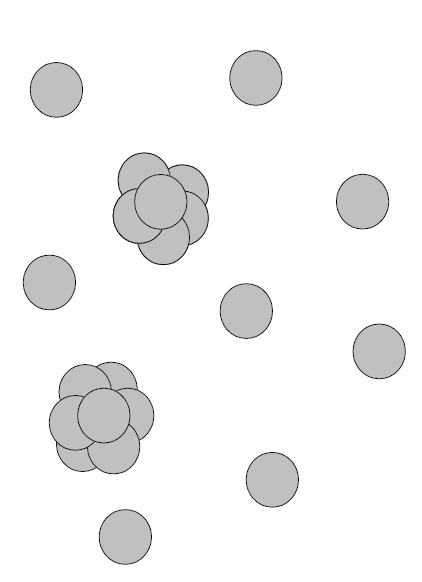
Figure 1: Gas as binary mixture.

Therefore it is possible to formulate the following basic assumption: elementary particles of gas (atoms or molecules) form small, relatively stable clusters consisting of $c$ particles each. Their concentration is a function of state. Thus, it immediately infers that the gas should be considered as (at least) two-component system (see Fig. 1).

The ground state of the system under consideration is expected to be a full separation as the energetically preferable one (we do not address here those special cases when geometry allows packing denser that FCC or HCP). On the other hand, at high temperature the system remains a mixture of atoms and clusters. Thus, at finite temperature the separation into two phases occurs.

This observation helps us to answer a very natural question: why do we suppose only one size clusters to be formed or, at least, to be stable. Unfortunately, we do not know an a priori reason for this. On the other hand, as one sees, the existence of clusters of one size leads to the separation. Therefore, the existence of clusters of any different number of particles would reveal itself through multiple separations. To the best of the author knowledge, it is not what happens in Nature with simple liquids. Thus, this a posteriori argument justifies our basic assumption. By the way, one may attribute complicated phase diagrams of complex liquids to the existence of clusters of different sizes and nature.

Such a model reveals a universal behaviour. Indeed, a close vicinity of the critical point (if it exists) has to be governed by the universal properties of the two-component mixture separation, regardless of the specific details of the inter-particle interaction. The latter affects the critical parameters, i.e. physical coordinates, but not the system’s behaviour.

Our basic assumption plays a role analogous to the Cooper pairing in the superconductivity theories: it is a microscopic phenomenon underlying the macroscopic one. Knowledge of the exact (probably, quantum) mechanism of this clustering is not crucial to understand the liquid-gas transition.

III Free Energy

We start with the expression for the Helmholtz free energy for a two-component slightly non-ideal gas mixture FoGu39

$$\beta F=N_{1}\ln\left(\frac{\lambda_{1}^{3}}{e}\frac{N_{1}}{V}\right)+N_{2}\ln\left(\frac{\lambda_{2}^{3}}{e}\frac{N_{2}}{V}\right)+\beta E_{B}N_{1}$$

$$\qquad\qquad+\frac{1}{V}\left(B_{11}N_{1}^{2}+2B_{12}N_{1}N_{2}+B_{22}N_{2}^{2}\right).$$ (1)

Let $N_{1}=n$ be the number of clusters containing $c$ particles each, $N_{2}=N-cn$ and $N$ is the total number of particles. $\beta=(k_{B}T)^{-1}$ as usual. As it said, we assume that all the clusters have the same and constant number of constituent particles, $c$. $\lambda_{i}=(2\pi\beta/m_{i})^{1/2}\hbar$ is a thermal wave length and $m_{i}$ is a particle mass. $E_{B}$ stands for a cluster binding energy and $B_{ij}$ denote second virial coefficients. Thus,

$$\beta F=n\ln\left(\frac{\lambda_{1}^{3}}{e}\frac{n}{V}\right)+(N-cn)\ln\left(\frac{\lambda_{2}^{3}}{e}\frac{N-cn}{V}\right)+\beta E_{B}n+\frac{1}{V}B(\beta;n),$$ (2)

and the internal energy

$$U=\left(\frac{\partial(\beta F)}{\partial\beta}\right)_{V}=\frac{3}{2}\frac{1}{\beta}[N-(c-1)n]+E_{B}n+\frac{1}{V}B^{\prime}_{\beta}(\beta;n),$$ (3)

where

$$B(\beta;n)\equiv B_{11}(\beta)n^{2}+2B_{12}(\beta)n(N-cn)+B_{22}(\beta)(N-cn)^{2}.$$ (4)

Within the same approximation (slightly non-ideal mixture) the equation of state reads FoGu39

$$P\beta=\frac{1}{V}[N-(c-1)n]+\frac{1}{V^{2}}B(\beta;n).$$ (5)

A dynamic equilibrium configuration of the two-component system is defined by the value of $n$ corresponding to the minimum of the total free energy. Simple differentiation of Eq. (2) leads to the main equation determining $n$:

$$\ln\left(\lambda_{1}^{3}\frac{n}{V}\right)-c\ln\left(\lambda_{2}^{3}\frac{N-cn}{V}\right)+\beta E_{B}+\frac{1}{V}B^{\prime}_{n}(\beta;n)=0,$$ (6)

or

$$\ln\left(\lambda^{3}x\rho\right)-c\ln\left(\lambda^{3}\rho(1-cx)\right)-{\textstyle\frac{3}{2}}\ln c+\beta E_{B}+\rho B^{\prime}_{x}(\beta;x)=0,$$ (7)

where $\rho\equiv N/V$, $x\equiv n/N$, $\lambda=\lambda_{2}$, $\lambda_{1}=c^{-1/2}\lambda$ and $B(\beta;x)=B_{11}x^{2}+2B_{12}x(1-cx)+B_{22}(1-cx)^{2}$.

One has to solve analytically Eq. (7), i.e. to find $x=x(\rho)$. Instead, we found an inverse function, $\rho=\rho(x)$, where $x\in[0,1/c]$. It is easily done with the aid of Lambert $W$-function CGHJK96Ha05 (another notation: $\omega$-function):

$$\lambda^{3}\rho=\left[\frac{ax}{(1-cx)^{c}}\right]^{\frac{1}{c-1}}\exp\left\{-W\left(-\left[\frac{ax}{(1-cx)^{c}}\right]^{\frac{1}{c-1}}\frac{B^{\prime}_{x}(\beta;x)}{(c-1)\lambda^{3}}\right)\right\},$$ (8)

where $a=c^{-3/2}\exp(\beta E_{B})$. In fact, the equation of state (5) in the form

$$P\beta=\rho[1-(c-1)x]+\rho^{2}B(\beta;x)$$ (9)

and Eq. (8) define $P(\rho)$ using the parameter $x$. The most interesting feature of Eq. (8) is the existence of ”forbidden” values for $\rho$. This behaviour is governed by the sign of the derivative $B^{\prime}_{x}(\beta;x)$. Namely, if for a given $\beta$ it remains negative for all permissible values of $x$, then $\rho$ ranges over the entire positive semi-axis. It is clear from the behaviour of Lambert function in the negative range CGHJK96Ha05 . If the expression changes its sign to positive, an equilibrium solution jumps from the $W_{0}$ branch, continued from positive argument, to the $W_{-1}$ one. Moreover, the positive range of the expression will have another ”forbidden” region as the absolute value of the Lambert function’s negative argument cannot exceed $1/\mathrm{e}$.

IV The Critical Point

The standard definition of a critical point is

$$\left(\frac{\partial P}{\partial\rho}\right)_{\beta}=\left(\frac{\partial^{2}P}{\partial\rho^{2}}\right)_{\beta}=0.$$ (10)

However, this definition is not applicable if one expects some singularity to be revealed at this point. Moreover, as we just saw, there exists some special behaviour characterized by the sign of $B^{\prime}_{x}(\beta;x)$. Thus, the very last (critical) point before the $\rho$-axis becomes “teared” up is defined by $B^{\prime}_{x}(\beta_{c};x_{c})=0$. In fact, this equation defines critical parameters: (inverse) critical temperature, $\beta_{c}$, and critical concentration, $x_{c}$, satisfying

$$[B_{12}(\beta_{c})-cB_{22}(\beta_{c})]+x_{c}[B_{11}(\beta_{c})-2cB_{12}(\beta_{c})+c^{2}B_{22}(\beta_{c})]=0.$$ (11)

The left-hand side consists of smooth monotonic functions of $\beta$ (second virial coefficients) and is linear in $x$ and, thus, attains its extremum at a limiting point. It cannot be $x_{c}=0$ because our physical system is supposed to be stable for small concentrations. Therefore, the only possibility is $x_{c}=1/c$ and Eq. (11) becomes

$$B_{11}(\beta_{c})-cB_{12}(\beta_{c})=0,$$ (12)

whose root, $\beta_{c}$, is the inverse critical temperature. Naturally, these equations for $x_{c}$ and $\beta_{c}$ are strongly approximation dependent ones. Higher viral expansion will complicate Eq. (11) leading to different values for the roots $x_{c}$ and $\beta_{c}$.

An important observation to make here is the atom-cluster ($B_{12}$) and the cluster-cluster ($B_{22}$) interactions should be substantialy weak in comparison with the inter-atomic ($B_{11}$) one, since part of the gas energy is accumulated in the cluster bindings. It results, in turn, in “shallow” potential well with a much shorter repulsive part and relatively small inter-cluster distance and, then, in a much higher density of a heavy component of the gas.

This new definition of the critical point, $B^{\prime}_{x}(\beta_{c};x_{c})=0$, allows one to write down an expansion in the vicinity of this point

$$B^{\prime}_{x}(\beta;x)\approx B^{\prime\prime}_{x\beta}(\beta_{c};x_{c})\Delta\beta+B^{\prime\prime}_{xx}(\beta_{c};x_{c})\Delta x,$$ (13)

where $\Delta\beta\equiv\beta_{c}-\beta$ and $\Delta x\equiv x_{c}-x$. Substituting this, $x\rightarrow\frac{1}{c}$, $\beta\rightarrow\beta_{c}$ and $1-cx\rightarrow c\Delta x$ into Eq. (7) we obtain the main Eq. (7) in a close vicinity of the critical point

$$c\ln\left(\Delta x\right)-cA=\rho B^{\prime\prime}_{xx}\Delta x,$$ (14)

where $cA\equiv\rho B^{\prime\prime}_{x\beta}\Delta\beta+\beta_{c}E_{B}-(c-1)\ln\left(\lambda_{c}^{3}\rho\right)+(c-{\textstyle\frac{5}{2}})\ln c$. This equation is solved as before with the aid of the Lambert function and its solution reads:

$$\Delta x=\mathrm{e}^{A}\exp\left\{-W\left({-\textstyle\frac{1}{c}}\rho B^{\prime\prime}_{xx}\mathrm{e}^{A}\right)\right\}$$ (15)

with $\mathrm{e}^{A}=\left(\lambda_{c}^{3}\rho\right)^{1-\frac{1}{c}}c^{1-\frac{5}{2c}}\exp{\left\{{\textstyle\frac{1}{c}}\left(\beta_{c}E_{B}+\rho B^{\prime\prime}_{x\beta}\Delta\beta\right)\right\}}$. This looks like an ultimate solution of the problem, at least, in the vicinity of the critical point but it does not account for the basic feature — the discontinuity of $\rho$-scale — and it should be used very carefully.

V Specific Heat

The internal energy is given by

$$\frac{U}{N}=\frac{3}{2}\frac{1-(c-1)x}{\beta}+E_{B}x+\rho B^{\prime}_{\beta}(\beta;x)$$ (16)

and the specific heat — by

$$c_{V}= \frac{\partial}{\partial T}\left(\frac{U}{N}\right)_{V}=-k_{B}\beta^{2}\frac{\partial}{\partial\beta}\left(\frac{U}{N}\right)_{\rho}$$

$$= k_{B}\left\{\textstyle{\frac{3}{2}}\left[1-(c-1)x\right]-\rho\beta^{2}B^{\prime\prime}_{\beta\beta}\right\}+k_{B}\beta\left\{\textstyle{\frac{3}{2}}(c-1)-\beta E_{B}-\rho\beta B^{\prime\prime}_{x\beta}\right\}x^{\prime}_{\beta}.$$ (17)

Therefore, if one looks for special behaviour of this quantity in the vicinity of the critical point then $x$ and $x^{\prime}_{\beta}$ have to be examined. We also make use of the fact that $c_{V}$ on the critical isohore behaves like $c_{p}$ in the second order phase transition. LanLif80

We start with substituting Eq. (13) into Eq. (8) and note that $B^{\prime\prime}_{xx}(\beta_{c};x_{c})=B_{11}(\beta_{c})-2cB_{12}(\beta_{c})+c^{2}B_{22}(\beta_{c})=B_{12}(\beta_{c})-cB_{22}(\beta_{c})$. It represents the cluster-atom and the cluster-cluster interactions which are supposed to be very small. Thus, one can expect existence of an interval where $B^{\prime}_{x}(\beta;x)\approx B^{\prime\prime}_{x\beta}(\beta_{c};x_{c})\Delta\beta$ and

$$\ln\left(\lambda_{c}^{3}\rho\right)=\ln\left[\frac{a_{c}/c}{(c\Delta x)^{c}}\right]^{\frac{1}{c-1}}-W\left(-\left[\frac{a_{c}/c}{(c\Delta x)^{c}}\right]^{\frac{1}{c-1}}\frac{B^{\prime\prime}_{x\beta}(\beta_{c};x_{c})}{(c-1)\lambda_{c}^{3}}\Delta\beta\right).$$ (18)

Further consideration depends on the sign of $B^{\prime\prime}_{x\beta}(\beta_{c};x_{c})\Delta\beta$. In the homogeneous phase it is negative and we are on the $W_{0}$ branch with a small positive argument. Here it is enough to take CGHJK96Ha05 $W_{0}(y)\approx y$ and subsequently

$$\lambda_{c}^{3}\rho=\left[\frac{a_{c}/c}{(c\Delta x)^{c}}\right]^{\frac{1}{c-1}}\left\{1-\left[\frac{a_{c}/c}{(c\Delta x)^{c}}\right]^{\frac{1}{c-1}}\frac{B^{\prime\prime}_{x\beta}(\beta_{c};x_{c})}{(c-1)\lambda_{c}^{3}}\Delta\beta\right\}.$$

The relevant root behaves as

$$\left[\frac{(c\Delta x)^{c}}{a_{c}/c}\right]^{\frac{1}{c-1}}\approx\frac{B^{\prime\prime}_{x\beta}(\beta_{c};x_{c})}{(c-1)\lambda_{c}^{3}}\Delta\beta\qquad\mbox{or}\qquad\Delta x\propto\left(\Delta\beta\right)^{1-\frac{1}{c}}.$$

It means that the derivative $\Delta x/\Delta\beta$ and therefore the specific heat will show here the famous dependence $c_{p}\propto\left(\Delta\beta\right)^{-\frac{1}{c}}$. In view of the previous suggestion, $c=13$, this exponent becomes $\alpha\approx 0.077$.

An analogous calculation cannot be done for a nonhomogeneous phase as an equilibrium solution does not exist in this region.

VI Conclusions

A model that explains basic features of the condensation is presented. A simple assumption of relative stability of only one type of clusters statistically emerging in the gas immediately leads to the first order phase transition (phase separation) at some finite temperature. It is experimentally observed as a condensation process.

It should be stressed that this model is by no means a simplified version of Fisher’s one. As much as the monogamy is not a simplified version of the polygamy and the monotheism is not a simplified version of the polytheism.

Mathematically, the condensation reveals itself as a forbidden density (volume) region. The density jumps from its gaseous value to the liquid one. No intermediate values are allowed. A correspondent region for the Van der Waals equation is a well-known S-shaped instability. It needs special auxiliary construction to be treated as a metastable state.

This paper presents a new concept of the critical point: it is a point of the density’s continuity failure. This definition coincides graphically with the old one but it allows to construct a convenient expansion in the close vicinity of the point under consideration. It demonstrates the famous singularity with the exponent $\alpha\approx 0.077$ that agrees excellently with known data.

References

- (1) Isihara A 1971 Statistical Physics (New York: Academic Press)
- (2) Langer J S 2000 Ann. Phys. 281 941–90
- (3) Fisher M E 1967 Physics 3 255–83
- (4) Haberland H 1994 Rare Gas Clusters Clusters of Atoms and Molecules Chem. Phys. 52 (Springer Verlag) p 374–95; Berry R S 1999 Phases and Phase Changes of Small Systems Theory of Atomic and Molecular Clusters (Springer Verlag) p 1–25
- (5) Mossa S and Tarjus G 2003 J. Chem. Phys. 119 8069–74
- (6) Karnicky J F, Reamer H H and Pings C J 1974 J. Chem. Phys. 64 4592–600; Kirstein B E and Pings C J 1976 J. Chem. Phys. 66 5730–6
- (7) Voronel A, to be published
- (8) Fowler R H and Guggenheim E A 1939 Statistical Thermodynamics (Cambridge)
- (9) Corless R M, Gonnet G H, Hare D E G, Jeffrey D J and Knuth D E 1996 Adv. Comput. Math. 5 329–59; Hayes B 2005 American Scientist Online http://www.americanscientist.org/template/IssueTOC/issue/701
- (10) Landau, L D, Lifshitz E M 1980 Statistical Physics (3rd Edition Part 1 ed.) Oxford: Pergamon, p. 515