Neuron dynamics in the presence of $1/f$ noise

Abstract

Interest in understanding the interplay between noise and the response of a non-linear device cuts across disciplinary boundaries. It is as relevant for unmasking the dynamics of neurons in noisy environments as it is for designing reliable nanoscale logic circuit elements and sensors. Most studies of noise in non-linear devices are limited to either time-correlated noise with a Lorentzian spectrum (of which the white noise is a limiting case) or just white noise. We use analytical theory and numerical simulations to study the impact of the more ubiquitous “natural” noise with a $1/f$ frequency spectrum. Specifically, we study the impact of the $1/f$ noise on a leaky integrate and fire model of a neuron. The impact of noise is considered on two quantities of interest to neuron function: The spike count Fano factor and the speed of neuron response to a small step-like stimulus. For the perfect (non-leaky) integrate and fire model, we show that the Fano factor can be expressed as an integral over noise spectrum weighted by a (low pass) filter function given by ${\cal F}(t,f)={\rm sinc}^{2}(\pi ft)$. This result elucidates the connection between low frequency noise and disorder in neuron dynamics. Under $1/f$ noise, spike dynamics lacks a characteristic correlation time, inducing the leaky and non-leaky models to exhibit non-ergodic behavior and Fano factor increasing logarithmically as a function of time. We compare our results to experimental data of single neurons in vivo [M.C. Teich, C. Heneghan, S.B. Lowen, T. Ozaki, and E. Kaplan, Journal of the Optical Society of America A 14, 529 (1997)], and show how the $1/f$ noise model provides much better agreement than the usual approximations based on Lorentzian noise. The low frequency noise, however, complicates the case for information coding scheme based on interspike intervals by introducing variability in the neuron response time. On a positive note, the neuron response time to a step stimulus is, remarkably, nearly optimal in the presence of $1/f$ noise. An explanation of this effect elucidates how the brain can take advantage of noise to prime a subset of the neurons to respond almost instantly to sudden stimuli.

I Introduction

One of the major puzzles of neuroscience is how neurons can store, process, and compute despite the fact that the brain is extremely noisy koch_book . Understanding the evolved mechanisms and the associated non-linear dynamics that allow the neurons to function in – and even exploit – a noisy environment is an essential step towards gaining insight into the information transmission and communication networks in the brain. Such studies also have important implications beyond the domain of biophysics and neuroscience. Noise provides a critical barrier for the development of sensitive electronic and mechanical devices, particularly at the nanoscale weissman88 ; kogan96 . Increasingly, researchers are focusing on exploring innovative, non-traditional device design and control strategies that exploit the ambient noise badzey05 ; almog07 ; murali09 ; guerra09 ; guerra10 ; zamora10 ; worschech10 ; fierens10 . In this regard, there are clear advantages to understanding how nature has managed to harness noise in a setting whose primary (apparent) function is to manage information.

It is generally accepted that neurons communicate with each other using sharp electric pulses referred to as action potentials or spikes. Each neuron is connected to several other neurons, and will only generate a spike output when the integrated input from other neurons exceeds a certain threshold gerstein64 ; hodgkin52 ; lapicque07 . A startling discovery that (under certain circumstances) neurons can spike more regularly when stimulated by noise longtin91 ; douglass93 ; mainen95 led to assertions that noise is inherent to neuron function. Several subsequent experimental and theoretical studies were aimed at elucidating the functionality of neural noise nozaki99b ; nozaki99a ; soma03 ; middleton03 ; rossum03 ; yu05 . In the first instance, noise – as expected – introduces a variability in the interspike intervals and degrades the information capacity of the spike trains, with low contrast signals being most affected rossum03 . At the same time, these studies also found that stochastic resonance provides a mechanism for neurons to take advantage of their own noise. In stochastic resonance, the addition of an appropriate amount of noise in a non-linear system can induce regularity by sensitizing subthreshold excitations, thus providing the extra energy for them to reach threshold longtin91 ; douglass93 ; nozaki99a and enabling their detection. Additionally, Brunel et al. brunel01 and Svirskis svirskis03 have shown that a model neuron, when subjected to low frequency noise, is able to respond faster to a sudden excitation than in the absence of noise. For an animal living in a natural environment, the ability to react quickly to sudden threats can mean the difference between life and death.

All of the studies to date that have considered the impact of low frequency noise on neurons tend to model noise characterized by a single Lorentzian power spectrum. Natural noise, however, has an ubiquitous $1/f$ frequency dependence kogan96 ; press78 ; voss75 ; hateren97 ; hausdorff96 ; diba04 . From current carrying electronic devices and geophysical time series to biological systems, the $1/f$ power spectrum is everywhere. In biological settings, human hearing and speech voss75 , the response of biological photoreceptors to large intensity variation of visual image streams in nature hateren97 , the stride intervals time series of normal human gait hausdorff96 , intrinsic noise in neuronal membranes due to stochastic opening and closing of the various ion channels diba04 , etc. all exhibit $1/f$ behavior. Guerra et al. guerra09 demonstrated how stochastic resonance induced by $1/f$ noise can increase the sensitivity of nanomechanical resonators, allowing for the possibility of fashioning them into noisy but robust nanoscale computation devices. Neither the response nor the details of the underlying non-equilibrium behavior that makes neurons robust to natural ($1/f$) noise is well understood.

In this paper, we present a comprehensive study of how neuron dynamics is affected by an arbitrary noise spectral density, and which sectors of the spectra are responsible for the beneficial functions that noise can provide. Specifically, we explore whether neuron response under $1/f$ noise is significantly different from the one found in the presence of a simple Lorentzian spectra.

The relevance of low frequency noise, implied by a $1/f$ spectrum, to spike dynamics at the single neuron level is especially evident, as we shall argue, in the direct experimental measurements of the spike count Fano factor by Teich et al.teich97 ; turcott95 (Fano factor is the ratio between the variance and the mean spike number during a given observation time). These authors demonstrated that the Fano factor of single neurons in the visual systems of cats and insects increases monotonically as a function of time. This is in dramatic contrast to the simple Poisson model (white noise), which leads to Fano factor equal to one at all times. The monotonic rise is also incompatible with models based on Lorentzian noise because the resulting Fano factor saturates at times longer than the inverse Lorentzian half width middleton03 ; schwalger08 . We show that the characteristic non-ergodicity of $1/f$ noise explains why the Fano factor never saturates in single neuron experiments. Moreover, the rate at which the Fano factor grows as a function of time is different for $1/f$ and Lorentzian.

In addition, we consider the effect of $1/f$ noise on the reaction time of a neuron in response to a sudden stimulus. We demonstrate that $1/f$ noise is nearly optimal for speeding up neuron response. We provide an explanation for this effect that sheds light on the mechanism of neuron adaptation to their noisy environment.

This paper is organized as follows. Section II describes our model for the neuron: the leaky integrate and fire (LIF) model of the neuron, and explains how we introduce $1/f$ noise and other spectral densities in this model. Section III describes an analytical theory and a set of numerical simulations of the neuron Fano factor as a function of time and compares our result to experiment teich97 . Particularly notable is our general expression Eq. (13) relating the Fano factor to an integral over low frequency noise weighted by an appropriate filter function. Section IV addresses the question of how noise can provide a mechanism for neurons to respond faster to a sudden stimulus. Section V provides our concluding remarks.

II The LIF model

From a biophysical perspective, the classical Hodgkin-Huxley model hodgkin52 and its contemporary variants represent the most realistic mathematical description of electrical response of a single neuron. Due to their intrinsic complexity, however, such models render the theoretical and computational analysis of neuronal and neural network dynamics exceedingly difficult. For this reason, most studies to date tend to reference the simpler spiking neuron models, of which the leaky integrate and fire (LIF) model gerstein64 ; lapicque07 that we adopt is one. The LIF model represents each neuron by an electrical circuit; when appropriate circuit parameters and features are chosen, the LIF model can reproduce quite similar dynamics to the one described by the more complex Hodgkin-Huxley model koch_book .

The LIF model consists of a capacitor $C$ in parallel with a resistor $R$; an injected continuous current $I(t)$ models the spike input from a large number of neighboring neurons. The neuron (or capacitor) voltage $V(t)$ is given by the circuit equation,

$$C\frac{dV(t)}{dt}+\frac{V(t)}{R}=I(t).$$ (1)

A spike is generated whenever the voltage across the capacitor reaches a certain threshold $V_{\rm{th}}$; after the spike is emitted, the neuron is reset to a zero voltage state. Note how the threshold rule for spike generation introduces non-linearity in the LIF model: Consider two input currents $I_{1}(t)$ and $I_{2}(t)$; a neuron subject to input $[I_{1}(t)+I_{2}(t)]$ will generally reach threshold faster than a neuron that is subject to either $I_{1}(t)$ or $I_{2}(t)$ only. Hence, the sum of outputs obtained from $I_{1}(t)$ and $I_{2}(t)$ applied separately is different from the output obtained from $[I_{1}(t)+I_{2}(t)]$. Also, the resistance $R$ plays an important role in the model: it allows charge to leak out, thus negating inputs received in the distant past. Neurons have the property that inputs long past have less effect than recent inputs; a sufficient amount of input must happen sufficiently rapidly for the neuron to fire.

The version of the LIF model that we are using has an additional feature that makes it more realistic: The introduction of a refractory time period $\tau_{r}$, which models the physical reset time for a neuron after emitting a spike. This prevents the neuron from receiving input for a time $\tau_{r}$ after spiking. Our choice for these circuit parameters are given in Table 1.

The presence of a leak and a refractory period makes the LIF neuron extremely hard to treat analytically schwalger08 . As a result, many theoretical studies have focused on the $R=\infty$ and $\tau_{r}=0$ limit, the so called perfect (non-leaky) integrate and fire model middleton03 ; lindner04 . This latter model is much easier to analyze but as we will demonstrate, the reduced complexity also leads to significantly different dynamics.

II.1 Introducing noise in the LIF model

We considered the LIF model subject to a noisy input current of the form

$$I(t)=\theta\left(I_{0}+I_{1}\eta(t)\right),$$ (2)

where $I_{0}$ is a (constant) bias current, $I_{1}$ is the noise amplitude, and $\theta(x)$ is the Heaviside step function: $\theta(x)=1$ for $x\geq 0$ and $\theta(x)=0$ for $x<0$; this ensures the current input represents the sum of spikes from a large number of connected neurons. The time series $\eta(t)$ is a Gaussian stochastic process, with variance equal to one and power spectra given by

$$\tilde{S}(f)=\frac{1}{2\pi}\int_{-\infty}^{\infty}dt\;\textrm{e}^{i2\pi ft}\langle\eta(t)\eta(0)\rangle,$$ (3)

with the brackets $\langle\quad...\quad\rangle$ denoting ensemble averages over a large number of time series $\eta(t)$. Appendix A describes the method used to generate individual time series for any given noise spectral density $\tilde{S}(f)$. We considered a number of different noise densities, including the family of power law spectral densities

$$\tilde{S}_{\alpha}(f)=A_{\alpha}\frac{1}{f^{\alpha}},$$ (4)

where $\alpha$ is an exponent ($\alpha=1$ corresponds to $1/f$ noise). The normalization constant $A_{\alpha}$ is set by the condition for the variance to be one, $2\pi\int df\tilde{S}(f)=\langle\eta^{2}\rangle=1$ [In the case of $\alpha=1$ Eq. (4) is valid for $\gamma_{\rm{min}}<f<\gamma_{\rm{max}}$; $\gamma_{\rm{min}}$ is a lower cut-off for which $\tilde{S}_{\alpha}(f)$ saturates, and $\gamma_{\rm{max}}$ is an upper cut-off for which $\tilde{S}_{\alpha}(f)$ goes to zero faster than $1/f^{2}$ – see below].

Another important class of noise spectral density arises when the environment fluctuates with a single characteristic time $\tau_{c}$:

$$\tilde{S}(f)=\frac{1}{2\pi^{2}}\frac{\gamma}{f^{2}+\gamma^{2}},$$ (5)

with $\gamma\equiv 1/(2\pi\tau_{c})$. This is a Lorentzian power spectrum and it implies $S(t)=\langle\eta(t)\eta(0)\rangle=\textrm{e}^{-|t|/\tau_{c}}$. Many authors refer to $\tau_{c}$ as the “correlation time”, and to the Lorentzian spectra as “time correlated noise”. In the limit that $\gamma$ goes to infinite ($\tau_{c}\rightarrow 0$), $\tilde{S}(f)\approx(2\pi^{2}\gamma)^{-1}$ is approximately constant for all $f\ll\gamma$. Hence $\gamma\rightarrow\infty$ is the “white noise” limit. Another important limit occurs when $\gamma\rightarrow 0$ ($\tau_{c}\rightarrow\infty$): In this case $\tilde{S}(f)\rightarrow\frac{1}{2\pi}\delta(f)$, signaling a “static” limit.

It is useful to recall the basic physical picture for the origin of $1/f$ noise. It emerges from the combination of a large number of Lorentzian fluctuators with an exponentially wide distribution of characteristic rates $\gamma$ kogan96 ; weissman88 . For example, assume $\gamma=\gamma_{\rm{max}}\textrm{e}^{-\lambda}$, with $\lambda$ a random variable that represents a distribution of activation energies. Assuming $\lambda$ is uniformly distributed in the interval $[0,\lambda_{\rm{max}}]$ we get

$$\tilde{S}(f) = \int_{0}^{\lambda_{\rm{max}}}\frac{d\lambda}{\lambda_{\rm{max}}}\frac{1}{2\pi^{2}}\frac{\gamma}{f^{2}+\gamma^{2}}$$

$$=\frac{1}{2\pi^{2}\lambda_{\rm{max}}}\int_{\gamma_{\rm{min}}}^{\gamma_{\rm{max}}}\frac{d\gamma}{\left|\frac{d\gamma}{d\lambda}\right|}\frac{\gamma}{f^{2}+\gamma^{2}}$$

$$= \frac{\arctan\left(\frac{\gamma_{\rm{max}}}{f}\right)-\arctan\left(\frac{\gamma_{\rm{min}}}{f}\right)}{2\pi^{2}\lambda_{\rm{max}}}\frac{1}{|f|}.$$

When $\gamma_{\rm{min}}\ll|f|\ll\gamma_{\rm{max}}$, we may approximate $\arctan(\gamma_{\rm{max}}/f)\approx\pi/2$ and $\arctan(\gamma_{\rm{min}}/f)\approx 0$; this leads to

$$\tilde{S}(f)\approx\frac{1}{4\pi\ln\left(\frac{\gamma_{\rm{max}}}{\gamma_{\rm{min}}}\right)}\frac{1}{|f|},$$ (7)

where we used the fact that $\lambda_{\rm{max}}=\ln(\gamma_{\rm{max}}/\gamma_{\rm{min}})$. Hence, overall the resultant noise is well described by

$$\tilde{S}(f)=\left\{\begin{array}[]{c c}\frac{A_{1}}{\gamma_{\rm{min}}}&0\leq|f|<\gamma_{\rm{min}}\\ \frac{A_{1}}{|f|}&\gamma_{\rm{min}}\leq|f|<\gamma_{\rm{max}}\\ 0&\gamma_{\rm{max}}\leq|f|<\infty\end{array}\right.,$$ (8)

with constant $A_{1}=\left[4\pi\ln\left(\gamma_{\rm{max}}/\gamma_{\rm{min}}\right)\right]^{-1}$.

From Eq. (II.1) we see that the distribution of Lorentzian linewidths $\gamma$ is given by $P(\gamma)=1/|d\gamma/d\lambda|=1/\gamma$. This is the reason why the spectrum acquires the $1/f$ dependence. We may generalize this distribution to $P(\gamma)=1/\gamma^{\alpha}$, with $\alpha$ a dimensionless exponent; carrying though a similar derivation as in Eq. (II.1) leads to $\tilde{S}(f)\propto 1/f^{\alpha}$. This shows that deviations of the $1/\gamma$ distribution will reflect directly into a $\alpha\neq 1$ exponent for the noise spectrum.

Usually, $\gamma_{\rm{min}}$ is exponentially small, and the experimental observation time window $T$ is smaller than $\gamma_{\rm{min}}^{-1}$. In this case the low frequency cut-off will be instead set by $\gamma_{\rm{min}}=T^{-1}$. As the observation time $T$ increases, more low frequency fluctuators will play a role; as a result, $1/f$ noise has no characteristic time scale, and displays non-ergodic behavior (time averages of observables are non-convergent, and can not be equivalent to ensemble averages). Below we discuss how the non-ergodic property leads to an increasing neuron Fano factor as a function of time.

II.2 White versus $1/f$ noise in the superthreshold regime: Bursting phenomena

To compare LIF dynamics under the effect of white and $1/f$ spectra, we considered noise in the superthreshold regime ($I_{0}>V_{\rm{th}}/R=4.28\times 10^{-10}$ A). We assumed $I_{0}=4.3\times 10^{-10}$ A, slightly above threshold, ensuring that without noise the neuron will spike every $46$ ms. For the cases with noise, we used $I_{1}=0.1I_{0}$. The algorithm of Appendix A was used to generate a current input $I(t)$, and Eq. (1) is integrated using the Runge-Kutta method. Figures 1(a) and 1(b) shows the neuron voltage as a function of time, for a particular time series (the observation time window was $T=2$ s). Under white noise, the spiking remains quite regular over time, because $I(t)$ varies rapidly and most of its fluctuating components are filtered out. On the other hand, $1/f$ noise shows a combination of long periods of inactivity, with the voltage taking a long time to reach threshold, together with periods of spike bursting where the voltage reaches threshold on a much shorter time scale. This is a result of the fact that under $1/f$ noise, the current tends to get “stuck” at either small or large values.

Table 1: Circuit parameters used in our LIF model. The parameters are similar to the ones used to describe neurons in the cat’s visual cortex (Chapter 14 of koch_book ).

Resistance	$R=38.3$ M$\Omega$
Capacitance	$C=0.207$ nF
Circuit time constant	$RC=7.93$ ms
Threshold voltage	$V_{\rm{th}}=16.4$ mV
Refractory period	$\tau_{r}=2.68$ ms

(a) White Noise

(b) $1/f$ Noise

Figure 1: (color online). Neuron voltage as a function of time (black curve), for (a) white noise and (b) $1/f$ noise. The vertical lines (red) denote spiking events. Note how $1/f$ noise leads to long time intervals with no spike generation, followed by intervals with spike bursting.

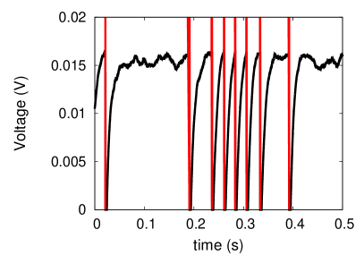
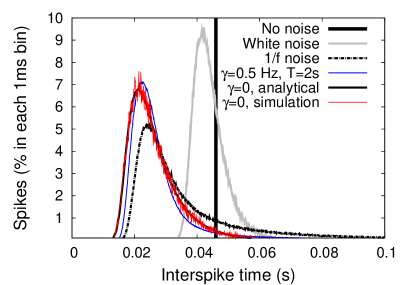
Figure 2 shows the interspike time interval histogram (ISI) for a 100,000 ensemble of time series with the same parameters considered in Figs. 1(a) and 1(b). Here we see that both types of noise can cause a notable decrease in the mean interspike time interval (compare to the noiseless case of a constant bias current). However, 1/$f$ noise leads to a far more dramatic shift. A large portion of the interspike time histogram lies significantly below the noiseless interval, and a long tail is observed at large interspike times. This behavior is characteristic of bursting (See e.g. Chapter 16 of koch_book ); several spikes occur in rapid succession, followed by a longer period without spike activity.

Figure  2 also shows the ISI for two Lorentzian noise spectra, with $\gamma=0$ Hz and $\gamma=1/T=0.5$ Hz, where $T=2$ s was the simulation time window for each time series. Lorentzian noise with such low frequency leads to an ISI that is nearly as broad as the $1/f$ noise case; however, the Lorentzian noise cases do not display the long time tail characteristic of $1/f$ noise. The simulations for $\gamma=0$ Hz can be compared to an exact analytical result obtained using the methods of Refs. middleton03 ; lindner04 (See Appendix B). Note how the $\gamma=0$ Hz simulations are in excellent agreement with the exact result.

Figure 2: (color online) Interspike interval histogram (ISI) for the cases of white and $1/f$ noise considered in Figs. 1(a) and 1(b), respectively. The noise amplitude was $I_{1}=0.1I_{0}$, with bias current $I_{0}$ slightly above threshold. Also shown is the case of no noise ($I_{1}=0$), and of Lorentzian noise with $\gamma=0$ Hz and $\gamma=1/T=0.5$Hz, where $T=2$ s was the simulation time window for each time series. Note how $1/f$ has much broader ISI, with a long time tail extending well beyond its mean interspike time.

III Neuron Fano factor under $1/f$ noise

III.1 Fano factor in the perfect integrate and fire model: Analytical results

The Fano factor is defined bykoch_book

$$F(t)=\frac{\langle\left[\Delta N(t)\right]^{2}\rangle}{\langle N(t)\rangle},$$ (9)

where the random variable $N(t)$ is the number of spikes generated from $t^{\prime}=0$ to $t^{\prime}=t$, and $\Delta N(t)=N(t)-\langle N(t)\rangle$. Hence, the Fano factor measures the amount of uncertainty in the spike train at a given time $t$. A noiseless spike train with identical interspike time intervals yields $F(t)=0$. In contrast, consider the case that the spike events are uniformly distributed in the interval $[0,t]$: In this case the probability for a spike event to happen during a time interval $[t^{\prime},t^{\prime}+\Delta t]$ is independent of $t^{\prime}$ and given by $\mu\Delta t$, where $\mu$ is the mean firing rate. Then the resulting $N(t)$ is a Poisson random variable uncorrelated in time (white noise) with $\langle N(t)\rangle=\langle(\Delta N)^{2}\rangle=\mu t$, leading to $F(t)=1$ at all times. In the presence of low frequency noise, $F(t)$ is known to become larger than one middleton03 ; schwalger08 .

The observation of a Fano factor much larger than one rules out the simple Poisson model, and suggests the presence of long time correlations in the data teich97 ; koch_book . Middleton et al. middleton03 derived an analytic expression for the Fano factor of the perfect ($R=\infty$) integrate and fire model subject to Lorentzian noise [Eq (5)]. At times much longer than the average interspike interval their result becomes

$$F_{\rm{Lor.}}(t)=\frac{\langle(\Delta I^{2})\rangle}{\langle I\rangle}\frac{2\tau_{c}}{CV_{\rm{th}}}\left[1-\frac{\tau_{c}}{t}(1-\textrm{e}^{-\frac{t}{\tau_{c}}})\right],$$ (10)

where $\langle(\Delta I^{2})\rangle=I_{1}^{2}$ is the current variance, $\langle I\rangle=I_{0}$ is the bias current, $\tau_{c}$ is the correlation time of the Lorentzian noise, $C$ is the capacitor’s voltage, and $V_{\rm{th}}$ is the threshold voltage. We emphasize that Eq. (10) assumes an input current $I(t)=I_{0}+I_{1}\eta(t)$, i.e., it neglects the step function used in our numerical computations [compare to Eq. (2)].

Here we generalize this result to an arbitrary noise spectral density. An RC circuit with no leakage ($R=\infty$) will lead to a capacitor voltage $V$ that always increases with increasing time. In the case of the neuron, $V$ is reset to zero when it reaches the threshold $V_{\rm{th}}$. In other words, the voltage is decreased by $V_{\rm{th}}$ each time the neuron spikes. An equivalent way to treat this reset process is to instead increase the threshold by an additional $V_{\rm{th}}$ each time the neuron spikes; this allows us to count the number of spikes at a given time $t$ by simply dividing the monotonically increasing $V$ by $V_{\rm{th}}$. Therefore the random variable $N(t)$ is well approximated by

$$N(t)\approx\frac{V(t)}{V_{\rm{th}}}=\frac{1}{CV_{\rm{th}}}\int_{0}^{t}dt^{\prime}I(t^{\prime}).$$ (11)

This approximation is valid at long times, $t\gg CV_{\rm{th}}/I_{0}$, i.e. times much longer than the mean interspike interval so that $N(t)$ can be represented by a real number instead of an integer.

The simplicity of the perfect integrate and fire model lies in the fact that we do not need to consider the threshold barrier explicitly. This property relies heavily on the fact that the voltage of an RC circuit never decreases when $R=\infty$. It is worthwhile to show how the approximation Eq. (11) fails in the presence of any amount of leakage.

When $R<\infty$, the mean voltage according to Eq. (1) is given by $RI_{0}(1-\textrm{e}^{-t/RC})$. Hence when $t\rightarrow\infty$ the mean voltage saturates at $RI_{0}$, and the approximation of Eq. (11) would give $\langle N(t\rightarrow\infty)\rangle=RI_{0}/V_{\rm{th}}<\infty$. This is clearly an unphysical result: If the neuron spikes at least once, it will spike an infinite number of times when $t\rightarrow\infty$, and $\langle N(t\rightarrow\infty)\rangle$ must be either $0$ or $\infty$. This unphysical saturation of $\langle N(t)\rangle$ shows why we must include the threshold barrier explicitly when dealing with the leaky model; it also shows why it is so difficult to treat the leaky model analytically.

In the absence of leakage, we have $\langle N(t)\rangle=t\;I_{0}/(CV_{\rm{th}})$, i.e. at long times the number of spikes increases indefinitely with increasing time. The Fano factor can be calculated explicitly plugging Eqs. (2) and (11) into Eq. (9),

$$F(t) = \frac{CV_{\rm{th}}}{I_{0}t}\frac{I_{1}^{2}}{(CV_{\rm{th}})^{2}}\int_{0}^{t}dt^{\prime}\int_{0}^{t}dt^{\prime\prime}\langle\eta(t^{\prime})\eta(t^{\prime\prime})\rangle$$ (12)

$$= \frac{2I_{1}^{2}}{CV_{\rm{th}}I_{0}}\frac{1}{t}\left[\int_{0}^{t/2}dT\int_{0}^{2T}d\tau S(\tau)\right.$$

$$\left.+\int_{t/2}^{t}dT\int_{0}^{2(t-T)}d\tau S(\tau)\right].$$

In the last step we changed the variables to $T=(t^{\prime}+t^{\prime\prime})/2$ and $\tau=(t^{\prime}-t^{\prime\prime})$, and used the symmetry $S(\tau)=S(-\tau)$. Eq. (12) provides an explicit relationship between the Fano factor and an arbitrary time correlation function. For example, upon inserting $S(\tau)=\textrm{e}^{-|\tau|/\tau_{c}}$ we recover Eq. (10) exactly.

A simpler expression can be derived by inserting $S(t)=2\pi\int df\textrm{e}^{-i2\pi ft}\tilde{S}(f)$ into Eq. (12):

$$F(t)=\frac{2\pi I_{1}^{2}}{CV_{\rm{th}}I_{0}}\;t\int_{-\infty}^{\infty}df\tilde{S}(f){\cal F}(t,f),$$ (13)

where we defined the filter function by

$${\cal F}(t,f)={\rm sinc}^{2}(\pi ft),$$ (14)

where ${\rm sinc}(x)=\sin{(x)}/x$ is the “unnormalized sinc function”. Hence the Fano factor can be expressed as an integral over low frequency noise; the filter function ${\cal F}(t,f)$ dictates how much noise is ”allowed in” at each given time $t$. Inspecting Eq. (14) shows that it acts as a low pass filter with bandwidth $\approx 1/(\pi t)$. In the limit $t\rightarrow\infty$, we have $ft\gg 1$ for all frequencies, and ${\cal F}\approx\delta(f)/t$. This leads to a useful result

$$F(t\rightarrow\infty)=\frac{2\pi I_{1}^{2}}{CV_{\rm{th}}I_{0}}\tilde{S}(0).$$ (15)

Therefore, the saturation of the Fano factor (or lack thereof) at long times is directly proportional to the amount of zero frequency noise.

We can use Eq. (12) to find the neuron Fano factor subject to $1/f$ noise. From Eq. (II.1) we know that the time correlation function for $1/f$ noise can be written as

$$S_{1/f}(t)=\frac{1}{\ln{\left(\frac{\gamma_{\rm{max}}}{\gamma_{\rm{min}}}\right)}}\int_{\gamma_{\rm{min}}}^{\gamma_{\rm{max}}}\frac{d\gamma}{\gamma}\textrm{e}^{-\gamma|t|}.$$ (16)

Hence the Fano factor for $1/f$ noise can be written as a weighted average of Lorentzian Fano factors,

$$F_{1/f}(t) = \frac{2I_{1}^{2}}{CV_{\rm{th}}I_{0}}\frac{1}{\ln{\left(\frac{\gamma_{\rm{max}}}{\gamma_{\rm{min}}}\right)}}\int_{\gamma_{\rm{min}}}^{\gamma_{\rm{max}}}\frac{d\gamma}{\gamma^{2}}\left[1-\frac{1}{\gamma t}\left(1-\textrm{e}^{-\gamma t}\right)\right]$$ (17)

$$\approx \frac{2I_{1}^{2}}{CV_{\rm{th}}I_{0}}\frac{1}{\ln{\left(\frac{\gamma_{\rm{max}}}{\gamma_{\rm{min}}}\right)}}\frac{t}{2}\left[\frac{(3-2C_{E})}{2}-\ln{\left(\gamma_{\rm{min}}t\right)}\right],$$

where $C_{E}=0.5772$ is the Euler-Mascheroni constant. The latter approximation is valid for $\frac{1}{\gamma_{\rm{max}}}\ll t\ll\frac{1}{\gamma_{\rm{min}}}=T$, where $T$ is the experimental time window. Hence $F_{1/f}(t)$ increases monotonically with increasing time, until it reaches a saturation value around $\sim T/\ln{(T)}$. This saturation value, however, is artifact of the finite length $T$ of the experiment; it diverges as $T\rightarrow\infty$, i.e., when longer data sets are acquired. This effect is a manifestation of the non-ergodicity of $1/f$ noise. In stark contrast, for an experimental window $T>\tau_{c}$, the Fano factor for the simple Lorentzian noise saturates at $F_{\rm{Lor.}}=2\tau_{c}I_{1}^{2}/(CV_{\rm{th}}I_{0})$, and remains at this value regardless of whether $T$ is increased further. Assuming that this behavior carries over to the Leaky model, it offers one way to determine whether the neuron noise is better described by $1/f$ or Lorentzian spectrum. The dependence of $F(t)$ on $t$ is another potential discriminator, as we shall see below.

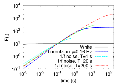
Figure 3 illustrates the relevance of the filter function Eq. (14) in quantifying the amount of noise absorbed by neurons at a given time $t$. Here we plot the Fano factor $F(t)$ for several different noise spectra, but choose each noise power (proportional to $I_{1}^{2}$) so that the Fano factor at a particular time $t=0.1$ s is identical [$F(0.1~{}{\textrm{s}})=10$] for all noise spectra. Hence at this particular $t=0.1$ s the amount of disorder on neuron response is the same even though we are describing neurons subject to very different dynamical environments. Nevertheless, at times after $t=0.1$ s the Fano factor differs considerably for different environments. This is a direct consequence of the fact that neurons integrate noise over a bandwidth $\approx 1/(\pi t)$; hence, as $t$ increases, a neuron absorbs noise over an increasingly narrow frequency range. Note also how $F(t)$ for $1/f$ noise depends on the total observation time window $T$, and how $F(t)$ is sensitive to different noise spectra before $t=0.1$ s.

Figure 3: (color online) Fano factor [Eq. (9)] for the case $R=\infty$ (non-leaky or perfect) integrate and fire model as a function of time for white noise, Lorentzian noise with $\gamma=0.16$ Hz, and $1/f$ noise with different observation time windows $T$. For each noise spectra, the noise amplitude $I_{1}$ was chosen so that $F(t=0.1{\textrm{~{}}s})=10$ for all noise spectra. This ensures that at $t=0.1$ s the neurons absorb the same amount of noise power, despite the fact that the noise spectra are quite different. Nevertheless, for times $t$ after $0.1$ s, the Fano factor differs considerably for different spectra. This occurs because neurons “integrate noise” over a bandwidth $\approx 1/(\pi t)$ as described by the filter function Eq. (14).

III.2 Fano factor in the perfect integrate and fire model: Numerical results

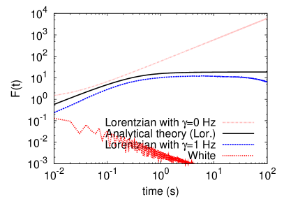
Figure 4 shows the Fano factor, as a function of time, for $I_{0}=I_{1}=2\times 10^{-10}$ A and $T=10^{2}$ s for white noise, and for Lorentzian noise with $\gamma=1$ Hz [$\tau_{c}=1/(2\pi)$ s] and $\gamma=0$ Hz ($\tau_{c}=\infty$). We also plot the analytical expression Eq. (10) for the $\gamma=1$ Hz Lorentzian Fano factor; as expected, the analytical expression shows slightly higher disorder [larger $F(t)$] than our Lorentzian noise simulation, because the latter only includes positive input currents (they are in close agreement when $I_{1}\ll I_{0}$). For white noise, the Fano factor tends to a small value at long times, in accordance with Eq. (15) that gives $F(t\rightarrow\infty)\propto 1/\gamma_{\rm{max}}$ ($\gamma_{\rm{max}}=10^{5}$ Hz is the upper frequency cut-off of our white noise spectrum). For the $\gamma=0$ Lorentzian, we have $F(t)\propto t$ in accordance with the limit $\tau_{c}\rightarrow\infty$ of Eq. (10).

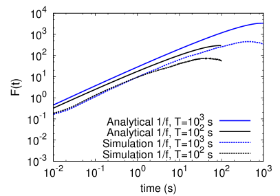
Figure 5 shows the neuron Fano factor subject to $1/f$ noise, using two different simulation time windows: $T=10^{2}$ s and $T=10^{3}$ s. We also show the corresponding analytic results using Eq. (17) with $\gamma_{\rm{min}}=T^{-1}$ and $\gamma_{\rm{max}}=N/T$ ($N$ is the number of frequency intervals used in our simulation, see Appendix A). Similar to the Lorentzian case, the analytic expressions for $F(t)$ are larger than the numerical results because the former does not take into account the step function in Eq. (2).

As expected, we find that the qualitative behavior of 1/$f$ noise is markedly different from Lorentzian noise. While for Lorentzian noise $F(t)$ increases linearly with $t$ until it reaches an asymptotic maximum at $t\approx\tau_{c}$, for $1/f$ noise $F(t)$ increases logarithmically [$\propto-t\ln{(t/T)}$] and only reaches a slight saturation when $t\approx T$, the maximum possible value of time.

Figure 4: (color online) Fano factor [Eq. (9)] for the $R=\infty$ (non-leaky or perfect) integrate and fire model as a function of time for white noise, Lorentzian noise with $\gamma=1$ Hz, and $\gamma=0$ Hz, the static case. We assumed $I_{0}=I_{1}=2\times 10^{-10}$ A and other parameters as in Table 1. Also shown is a comparison between the numerical simulation and the analytical expression Eq. (10) for Lorentzian noise. For white noise, $F(t)$ tends to a quite small value at long times; for Lorentzian noise, $F(t)$ plateaus at times $t\approx(2\pi\gamma)^{-1}$.

Figure 5: (color online) Fano factor [Eq. (9)] for the non-leaky (perfect) integrate and fire model as a function of time for $1/f$ noise, using the same parameters as in Fig. 4. We show simulations of $1/f$ noise for two different time series: $T=10^{2}$ s and $T=10^{3}$ s, where $T$ is the length of the simulation time window. We also show the corresponding analytical approximations Eq. (17). Note how the Fano factor due to $1/f$ noise increases logarithmically until it reaches a slight saturation at $t=T$, the “maximal experimental time”. This behavior agrees qualitatively to what is observed in measurements on single visual neurons in cats and insects teich97 .

III.3 Fano factor in the leaky integrate and fire model

We now describe the impact of leakage on the Fano factor. We simulated the LIF model under Lorentzian and $1/f$ noise of several different noise levels. Figure 6 compares the Fano factor with leakage and without leakage; in every case, leakage increases the Fano factor noticeably (i.e. there is increased variability in the spike train). This happens because in the presence of leakage, the neuron tends to forget past inputs that were not strong enough to break the threshold barrier and returns to its rest state even though it received a considerable amount of subthreshold input. This situation is dramatically different from the perfect (non-leaky) model: In the absence of leakage, every subthreshold stimulation increases the charge of the neuron, priming it for firing. The quantitative difference in Fano factor highlights the importance of leakage in neuron dynamics. For example, note the dramatic quantitative difference between Fano factor for leaky and non-leaky cases at the level of 1% of $1/f$ noise ($I_{1}/I_{0}=0.01$).

(a) Lorentzian Noise, $\gamma=1$ Hz

(b) 1/$f$ Noise, $T=100$ s

Figure 6: (color online) Fano factor for integrate and fire neuron with leakage and without leakage, for $I_{1}/I_{0}=1,0.1,0.01$. Leakage increases the Fano factor considerably, and can produce large quantitative difference at low levels of noise.

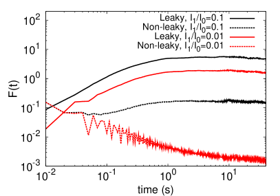
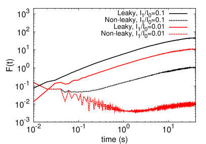
Our explicit numerical results of Fano factor subject to $1/f$ noise shows that $F(t)$ does not saturate at long times. This property is consistent with the the direct measurements of neuron Fano factor presented in Teich et. al. (See Fig. 6 in teich97 ). Their experimental Fano factor increases well beyond one, and does not appear to reach a plateau at long times. Note that previous calculations based on Lorentzian noise middleton03 ; schwalger08 have showed that the Fano factor saturates at long times. This result is independent of whether one uses the perfect or the leaky integrate and fire model.

One can argue that with respect to a Lorentzian noise model, the experimental data only explicitly rules out cases with $\tau_{c}<T$, i.e. Lorentzian models with correlation time longer than the experimental window will not show saturation. This is true, but the Lorentzian and $1/f$ model predictions for $F(t)$ differ in other respects as well, which do not depend on $\tau_{c}$ or $T$.

The Fano factor $F(t)$ for the experimental data has a tangent slope of $0.4-0.5$ around $t\sim 1$ s in log-log plot (Fig. 6 of teich97 ). The predicted slope of the Lorentzian Fano factor, however, is $1$ for $t\ll\tau_{c}$ (before saturation takes place). This difference rules out the possibility that the experimental results can be understood in terms of an unsaturated Lorentzian model.

The Fano factor under $1/f$ noise has a tangent slope of approximately $0.7$ around $t\sim 1$ s (Figs. 5 and 6b). Note that the Fano factor increases logarithmically, so the exponent depends on particular time $t$ chosen to measure the slope. We repeated our simulation using $1/f^{0.6}$ noise, and obtained results very similar to Figs. 5 and 6b, except that the slope was reduced to $\approx 0.5$. This shows that a LIF model subject to $1/f^{\alpha}$ noise can provide an excellent fit to experimental data of long time neuron dynamics, and further suggests that neuron input noise is better approximated by a $1/f$-like spectrum, than a Lorentzian with a single characteristic correlation time.

IV How neurons respond to a sudden step excitation

We now analyze the impact of low frequency noise on the reaction time of a LIF neuron. We consider the reaction of a neuron subject to the following stimulus,

$$I(t)=\theta\left(I_{1}\eta(t)+I_{0}\theta(t-t_{\rm{step}})\right).$$ (18)

For times between $t=0$ and $t=t_{\rm{step}}$, the current input is pure noise with subthreshold amplitude $I_{1}$; at $t=t_{\rm{step}}$, a superthreshold bias current $I_{0}$ is suddenly turned on in addition to the noise. In the simulations below we used $t_{\rm{step}}=1.5$ s, $I_{0}=4.3\times 10^{-10}$ A, and $I_{1}=0.3I_{0}$. Figure 7 shows the mean fire rate averaged on $1$ ms bins after 100,000 time series are taken into account. The ensemble of time series can be thought of either an actual ensemble of different neurons or to a single neuron subject to statistically similar excitations at different times. In both cases, we can make claims of optimality on “average”.

Figure 7: (color online) Mean fire rate of single neuron in response to step excitation under various types of noise: Lorentzian noise with $\gamma=0$ Hz (“static” case), Lorentzian noise with $\gamma=1000$ Hz, white noise, and $1/f$ noise. We also included the noiseless case for comparison. The presence of noise primes the neurons to react significantly faster. The reaction time is optimal (almost instantaneous) for the “static” case. Surprisingly, under $1/f$ noise the neuron response time is nearly optimal.

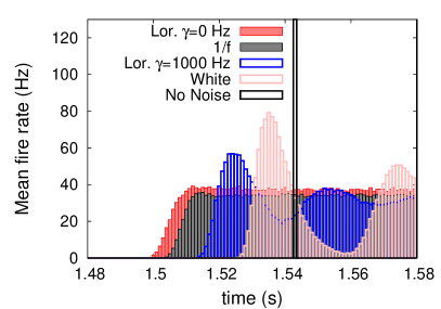
In the absence of noise, the LIF neuron takes $43$ ms to respond. The quickest response is obtained in the case of Lorentzian noise with $\gamma=0$ Hz, that is equivalent to $\tilde{S}(f)=\delta(f)/(2\pi)$, the static limit discussed in section II.1. Note that in this case the noisy current does not change in time, and is equivalent to a bias current with amplitude picked from a Gaussian distribution. The response under $1/f$ noise lags behind the static case by only $\approx 5$ ms, i.e., it is nearly optimal. Both static and $1/f$ noise reach their steady state much faster when compared to other types of noise. Lorentzian noise with roll-off frequency $\gamma=1000$ Hz is intermediate between white and $1/f$ noise. Clearly, the response time improves as the noise gets dominated by low frequency components.

Figure 8: (color online) Histogram of first spike times under a step excitation subject to various types of noise. In the case of white noise, it takes $30$ ms for 1% of the neurons to spike for the first time. The situation is markedly different for the static case (Lorentzian with $\gamma=0$ Hz) and for $1/f$ noise. Here some neurons respond almost immediately, while others take a long time to spike; note the long time tail in the distributions for Lor. 0 Hz and $1/f$ noise.

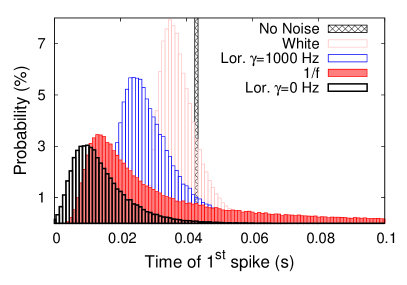
In order to elucidate the mechanism by which noise sensitizes neuron response time, we present two additional figures. Figure 8 shows a histogram of first spike times. Under white noise conditions, it takes approximately $30$ ms for 1% of the neurons to spike for the first time. On the other hand, it takes only $8$ ms for 1% of the $1/f$ noise neurons to spike and a mere $2.5$ ms for 1% of static noise (i.e. Lorentzian $\gamma=0$) neurons to spike for the first time. Neurons subject to $1/f$ noise and the $\gamma=0$ static noise have a much wider distribution of first spike times. Some neurons spike almost immediately, while others take a long time to spike – note the extended tail in the distributions. This broad distribution implies a greater variability in the neuronal interspike interval and a degradation of any information coded therein. Extreme low frequency noise ($1/f$ and $\gamma=0$) result in a trade off between reliability and rapid response.

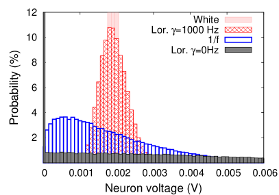
Figure 9 sheds light on the origin of this effect, by plotting the distribution of neuron voltages just before the step stimulus is applied. Here we see why the static case is optimal: The distribution of neuron voltages is nearly flat, and extends close to threshold. Hence, when the stimulus is applied, a significant amount of “primed neurons” will reach threshold almost instantly. While the voltage distribution for $1/f$ noise is not flat, it is broad and extends all the way to high voltages. Similar to the static case, the presence of a tail extending near threshold implies that a significant number of neurons are “primed” by $1/f$ noise; these neurons will react nearly instantly to the stimulus.

We note in passing that it is possible to engineer a Lorentzian noise spectrum to yield a response time similar to that for $1/f$ noise via an appropriate choice of $\gamma=1/T$, where we recall that $T$ is the simulation time window. For $T=2$ s, we find that $\gamma=0.5$ Hz does the trick, in agreement with expectations based on our previous analysis of the distribution of interspike time intervals for different conditions (c.f. Fig. 2): The shortest interspike time interval for a Lorentzian with $\gamma=0.5$ Hz is similar to that for $1/f$ noise. The two distributions are not identical. The ISI for the $1/f$ has a tail that extends to much longer times.

Figure 9: (color online) Neuron voltage right before the step excitation arrives. Note that for the static case (Lor. 0 Hz) and for the $1/f$ noise case, a significant fraction of neurons have quite high voltage. Hence these neurons will reach threshold much faster, explaining how noise can “prime” neurons for a fast response time.

V Conclusions

In conclusion, we presented analytical and numerical calculations of the perfect and the leaky integrate and fire neuron aimed at elucidating the impact of $1/f$ noise on single neuron dynamics. Though more difficult to analyze than the perfect integrate and fire model that is commonly used in noise and network studies, our LIF model is a more realistic model of a neuron and as we have shown, the inclusion of the “leakiness” gives rise to much higher disorder.

With regard to the response of the LIF to $1/f$ noise, we find a surprising dichotomy: While it degrades the ability to transmit information using interspike times, it manages to enhance the overall response time (of an ensemble of neurons) to a sudden stimulus by ensuring that a subset of neurons are primed with a near threshold voltage.

Our explicit numerical simulations of neuronal response to a sudden step excitation elucidates the mechanism by which noise can enhance neuron response time. Neuron response times were shown to be optimal under static noise (noise sharply peaked at zero frequency) because a large number of neurons are close to threshold just before the step stimulus arrives. This select group of neurons act as the alarm bells: They respond almost instantly to the step stimulus. Remarkably, as we demonstrated, the case of $1/f$ noise is not much different; the distribution for neuron voltages just before stimulus also has a long tail extending towards threshold. These results allude to a possible explanation for why the brain is populated by an astronomically large number of neurons. It may well be an evolutionary adaptation designed to take advantage of the ambient noise to enhance the probability of survival. Neuron redundancy enables faster response times in the presence of low frequency noise, which in turn allows an animal to react quickly to a sudden danger.

However, the apparently beneficial feature noted above does not come without cost. The $1/f$ noise trades off speed for reliability by introducing much more variability in the properties of the resulting spike train. We quantify this uncertainty using the Fano factor. Our analysis of the Fano factor reveals that in the presence of $1/f$ noise, this measure of disorder increases logarithmically as a function of time. On a positive note, we find an excellent qualitative agreement between Fano factor for the $1/f$ noise and the Fano factor derived from laboratory results of experiments with single neurons teich97 ; turcott95 . Specifically, the latter also rises monotonically well beyond one and shows no evidence for saturation. This agreement suggests that the neuron input noise is better approximated by a scale-free $1/f$-like spectrum than the more commonly invoked low frequency Lorentzian spectrum.

The rate at which the Fano factor for a Lorentzian spectrum grows with time prior to saturation is $F(t)\propto t$, independent of $\gamma$. Moreover, the Lorentzian Fano factor always tends to a plateau at long times middleton03 ; schwalger08 . Both tendencies are at odds with the behavior of the experimentally measured Fano factor regardless of whether the Lorentzian spectrum is fine-tuned to yield a response time similar to that of $1/f$ noise. We note that these claims can be definitively tested by repeating the experiments of Teich et al.teich97 with increasingly longer experimental time windows $T$.

The logarithmically rising Fano factor reflects the fact that the long time spike dynamics is dominated either by periods of extended inactivity or by periods of aggressive bursting. This behavior is due to the lack of ergodicity in $1/f$ noise, i.e., the fact that it lacks a characteristic correlation time. Not surprisingly, therefore, the neuron dynamics in the presence of $1/f$ noise is very different from that due to Lorentzian noise. As an aside, we note that the degree of uncertainty is also substantially greater in the leaky model than in the non-leaky (perfect) case.

These conclusions are consistent with the observation that some neurons seem to spike in a very irregular fashion. The temporal gaps of a spike train has much larger information capacity and for this reason, there is considerable body of work arguing that neurons use the timing intervals to encode information. Loss of reliability due to low frequency noise, however, limits the information capacity of the spike trains rossum03 . On the other hand, research has shown that in certain cases neurons can spike with high degree of reproducibility steveninck97 . Whether the origin of highly reproducible spike patterns is due to extremely low noise at the single neuron level, or due to a network effect that compensates for the noise remains to be seen. A more interesting possibility is that the various functional regions of the brain may have evolved different strategies for managing ambient noise, depending on function and associated information capacity demands.

Appendix A Numerical simulation of Gaussian noise with arbitrary spectral density

To simulate the noise used in Eq. (2) we used a variation of the efficient algorithm proposed by Timmers and Koenig timmer95 . Consider the time window from $t=0$ to $t=T$. Define a discrete set of $N$ time instants $t_{m}=n\Delta t/2$, where $n=0,1,\ldots,2N-1$ and $\Delta t=T/N$. Choosing $N$ as a power of $2$ allows the use of the fast Fourier transform algorithm, with significant speed up. The associated set of “lower half” frequencies are $f_{m}=m/T$, with $m=0,1,\ldots,N$, and the “upper half frequencies” are $f_{m}=(2N-m)/T$ for $m=N+1,N+2,\ldots,2N-1$. We are now ready to state the algorithm that generates individual real-valued time series $\eta(t_{m})$ ($\tilde{\eta}(f)$ are their Fourier transforms):

1. Set $\tilde{\eta}(f_{0})=0$;

2. For each $m=1,\ldots,N-1$, set $\tilde{\eta}=\textrm{e}^{i\pi r_{m}}\sqrt{\tilde{S}(f_{m})}$, where $r_{m}$ is a random number in the interval $[0,1)$;

3. Set $\tilde{\eta}(f_{N})=\sqrt{\tilde{S}(f_{N})}$;

4. Set $\tilde{\eta}(f_{N+m})$ equal to the complex conjugate of $\tilde{\eta}(f_{N-m})$ for all $m=1,\ldots,N$;

5. Finally, take the inverse Fourier transform of $\tilde{\eta}(f_{m})$. The resulting $\eta(t_{m})$ realizes an individual time series of the Gaussian process with noise spectrum $\tilde{S}(f_{m})$.

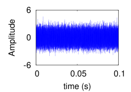
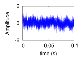
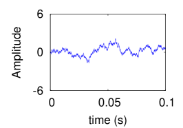
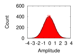
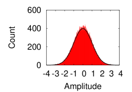
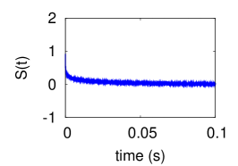
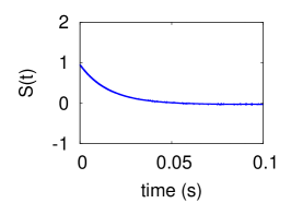
Figure 10 depicts three example time series: white noise, $1/f$ noise, and Lorentzian with half-width $\gamma=10$ Hz. We simulated 100,000 of these time series and studied their amplitude distribution and noise spectra [Eq. (3)]. Figure 11 demonstrates that the noise amplitudes are distributed according to a Gaussian, and Fig. 12 computes the ensemble average of their correlation function, $S(t)=\langle\eta(t)\eta(0)\rangle$. The latter have the expected forms: For white noise, $S(t)=\sin{(2\pi\gamma_{\rm{max}}t)}/(2\pi\gamma_{\rm{max}}t)$, for $1/f$ noise, $S(t)\approx 1-[C_{E}+\rm{ln}(\gamma_{\rm{max}}t)]/\rm{ln(\gamma_{\rm{max}}/\gamma_{\rm{min}})}$ ($C_{E}=0.5772$ is the Euler-Mascheroni constant), and $S(t)=\textrm{e}^{-\gamma t}$ for Lorentzian noise.

(a) White Noise

(b) 1/$f$ Noise

(c) Lorentzian Noise, $\gamma=10$ Hz

Figure 10: (color online) Example time Series for three different kinds of noise spectra.

(a) White Noise

(b) 1/$f$ Noise

(c) Lorentzian Noise, $\gamma=10$ Hz

Figure 11: (color online) Histogram for the amplitudes of $\eta(t)$ for 100,000 time series, demonstrating that $\eta(t)$ is Gaussian distributed.

(a) White Noise

(b) 1/$f$ Noise

(c) Lorentzian Noise, $\gamma=10$ Hz

Figure 12: (color online) Ensemble average correlation function, $S(t)=\langle\eta(t)\eta(0)\rangle$, calculated as an arithmetic average of several time series generated by the method.

Appendix B Exact calculation of the interspike interval histogram for the LIF model subject to static noise

The case of static noise $\tilde{S}(f)=\delta(f)/2\pi$ (a Lorentzian with $\gamma\rightarrow 0$) is particularly simple because the stochastic process $\eta(t)$ randomizing the current Eq. (2) does not change in time. Each $\eta$ is picked from a Gaussian distribution at $t=0$,

$$p(\eta)=\frac{1}{\sqrt{2\pi}}\textrm{e}^{-\frac{1}{2}\eta^{2}}.$$ (19)

As a result, the quasi-static method for calculating the ISI distribution developed in Refs. middleton03  and lindner04 becomes exact. As we show below, this allows us to compute the ISI distribution exactly even in the presence of leakage ($R<\infty$).

In the presence of leakage, the voltage is obtained by solving Eq. (1) under a constant current $I=I_{0}+I_{1}\eta$,

$$V(t)=R(I_{0}+I_{1}\eta)\left(1-\textrm{e}^{-\frac{t}{RC}}\right).$$ (20)

The interspike time interval $l$ will be given by the time it takes for this voltage to reach $V_{\rm{th}}$, leading to

$$l=\tau_{r}-RC\ln{\left(1-\frac{V_{\rm{th}}/R}{I_{0}+I_{1}\eta}\right)},$$ (21)

where $\tau_{r}$ is the refractory time period. The ISI distribution can now be computed from the expression

$$P(l)=\frac{1}{N_{\eta}}\int_{-\infty}^{\infty}d\eta p(\eta)\delta\left[l-\left(\tau_{r}-RC\ln{\left(1-\frac{V_{\rm{th}}/R}{I_{0}+I_{1}\eta}\right)}\right)\right],$$ (22)

where the normalization factor

$$N_{\eta}=\int_{\left[V_{\rm{th}}/(RI_{1})-I_{0}/I_{1}\right]}^{\infty}d\eta p(\eta)$$ (23)

ensuring that $\eta$ is strong enough to “click” the delta function. After some algebra we obtain the following exact result:

$$P(l)=\frac{CV_{\rm{th}}}{\sqrt{2\pi}I_{1}N_{\eta}}\frac{\textrm{e}^{-\frac{(l-\tau_{r})}{RC}}\textrm{e}^{-\frac{1}{2}\left(\frac{I_{0}}{I_{1}}\right)^{2}\left[1-\frac{CV_{\rm{th}}/I_{0}}{RC\left(1-\textrm{e}^{-\frac{(l-\tau_{r})}{RC}}\right)}\right]^{2}}}{\left[RC\left(1-\textrm{e}^{-\frac{(l-\tau_{r})}{RC}}\right)\right]^{2}}.$$ (24)

This expression is plotted in Fig. 2.

References

- (1) C. Koch, Biophysics of Computation: Information processing in single neurons (Oxford University Press, Oxford, UK, 1999).
- (2) M.B. Weissman, Rev. Mod. Phys. 60, 537 (1988).
- (3) Sh. Kogan, Electronic Noise and Fluctuations in Solids (Cambridge University Press, Cambridge, 1996).
- (4) R.L. Badzey and P. Mohanty, Nature 437, 995 (2005); A.R. Bulsara, ibid. 437, 962 (2005).
- (5) R. Almog, S. Zaitsev, O. Shtempluck, and E. Buks, Appl. Phys. Lett. 90, 013508 (2007).
- (6) K. Murali, S. Sinha, W.L. Ditto, and A.R. Bulsara, Phys. Rev. Lett. 102, 104101 (2009).
- (7) D.N. Guerra, T. Dunn, and P. Mohanty, Nano Letters 9, 3096 (2009).
- (8) D.N. Guerra, A.R. Bulsara, W.L. Ditto, S. Sinha, K. Murali and P. Mohanty, Nano Letters 10, 1168 (2010).
- (9) J. Zamora-Munt and C. Masoller, Optics Express 18, 16418 (2010).
- (10) L. Worschech, F. Hartmann, T.Y. Kim, S. Höfling, M. Kamp, A. Forchel, J. Ahopelto, I. Neri, A. Dari, and L. Gammaitoni, Appl. Phys. Lett. 96, 042112 (2010).
- (11) P.I. Fierens, S.A. Ibáñes, R.P.J. Perazzoa, G.A. Pattersonb and D.F. Grosza, Phys. Lett. A 374, 2207 (2010).
- (12) G.L. Gerstein and B. Mandelbrot, Biophys. J. 4, 41 (1964).
- (13) A. L. Hodgkin and A. F. Huxley, J. Physiol. 117, 500 (1952).
- (14) L. Lapicque, J. Physiol. Paris 9, 620 (1907).
- (15) A. Longtin, A. Bulsara, and F. Moss, Phys. Rev. Lett. 67, 656 (1991).
- (16) J.K. Douglass, L. Wilkens, E. Pantazelou, and F. Moss, Nature 365, 337 (1993).
- (17) Z.F. Mainen and T.J. Sejnowski, Science 268, 1503 (1995).
- (18) D. Nozaki, D.J. Mar, P. Grigg and J.J. Collins, Phys. Rev. Lett. 82, 2402 (1999).
- (19) D. Nozaki, J.J. Collins, and Y. Yamamoto, Phys. Rev. E60, 4637 (1999).
- (20) R. Soma, D. Nozaki, S. Kwak, and Y. Yamamoto, Phys. Rev. Lett. 91, 078101 (2003).
- (21) J.W. Middleton, M.J. Chacron, B. Lindner, and A. Longtin, Phys. Rev. E68, 021920 (2003).
- (22) M.C.W. van Rossum, B. J. O’Brien and R. G. Smith, J Neurophysiol, 89, 2406 (2003).
- (23) Y. Yu, R. Romero, and T.S. Lee, Phys. Rev. Lett. 94, 108103 (2005).
- (24) N. Brunel, F.S. Chance, N. Fourcaud, and L.F. Abbott, Phys. Rev. Lett. 86, 2186 (2001).
- (25) G. Svirskis, Nonlinear Analysis: Modelling and Control, 8, 77 (2003).
- (26) W.H. Press, Comments on Astrophysics 7, 103 (1978)
- (27) R.F. Voss, and J. Clarke, Nature (London) 258, 317 (1975).
- (28) J. H. van Hateren, Vision Research 37, 3407 (1997).
- (29) J. M. Hausdorff, P. L. Purdon, C. -K. Peng, Z. Ladin, J. Y. Wei, and A. L. Goldberger, J. Appl. Physiol. 80, 1448 (1996).
- (30) K. Diba, H.A. Lester, C. Koch, J. Neurosci. 24, 9723 (2004).
- (31) M.C. Teich, C. Heneghan, S.B. Lowen, T. Ozaki, and E. Kaplan, J. Opt. Soc. Am. A 14, 529 (1997).
- (32) R.G. Turcott, P.D.R. Barker, and M.C. Teich, J. Stat. Comp. Simul. 52, 253 (1995).
- (33) T. Schwalger and L. Schimansky-Geier, Phys. Rev. E77, 031914 (2008).
- (34) B. Lindner, Phys. Rev. E69, 022901 (2004).
- (35) R.R. de Ruyter van Steveninck, G.D. Lewen, S.P. Strong, R. Koberle, and W. Bialek, Science 275, 1805 (1997).
- (36) J. Timmer and M. Koenig, Astron. Astrophys. 300, 707 (1995).