On the Estimation of Coherence

Abstract

Low-rank matrix approximations are often used to help scale standard machine learning algorithms to large-scale problems. Recently, matrix coherence has been used to characterize the ability to extract global information from a subset of matrix entries in the context of these low-rank approximations and other sampling-based algorithms, e.g., matrix completion, robust PCA. Since coherence is defined in terms of the singular vectors of a matrix and is expensive to compute, the practical significance of these results largely hinges on the following question: Can we efficiently and accurately estimate the coherence of a matrix? In this paper we address this question. We propose a novel algorithm for estimating coherence from a small number of columns, formally analyze its behavior, and derive a new coherence-based matrix approximation bound based on this analysis. We then present extensive experimental results on synthetic and real datasets that corroborate our worst-case theoretical analysis, yet provide strong support for the use of our proposed algorithm whenever low-rank approximation is being considered. Our algorithm efficiently and accurately estimates matrix coherence across a wide range of datasets, and these coherence estimates are excellent predictors of the effectiveness of sampling-based matrix approximation on a case-by-case basis.

1 Introduction

Large-scale datasets are becoming more and more prevalent for problems in a variety of areas, e.g., computer vision, natural language processing, computational biology. However, several standard methods in machine learning, such as spectral clustering, manifold learning techniques, kernel ridge regression or other kernel-based algorithms do not scale to such orders of magnitude. For large datasets, these algorithms would require storage and operation on matrices with thousands to millions of columns and rows, which is especially problematic since these matrices are often not sparse. An attractive solution to such problems involves efficiently generating low-rank approximations to the original matrix of interest. In particular, sampling-based techniques that operate on a subset of the columns of the matrix can be effective solutions to this problem, and have been widely studied within the machine learning and theoretical computer science communities (Frieze et al., , 1998; Drineas et al., , 2006; Williams and Seeger, , 2000; Kumar et al., , 2009b). In the context of kernel matrices, the Nyström method (Williams and Seeger, , 2000) has been shown to work particularly well in practice for various applications ranging from manifold learning to image segmentation (Fowlkes et al., , 2004; Talwalkar et al., , 2008).

A crucial assumption of these algorithms involves their sampling-based nature, namely that an accurate low-rank approximation of some matrix ${\mathbf{X}}\in\mathbb{R}^{n\times m}$ can be generated exclusively from information extracted from a small subset ($l\ll m$) of its columns. This assumption is not generally true for all matrices, and explains the negative results of Fergus et al., (2009). For instance, consider the extreme case:

$${\mathbf{X}}=\left[\begin{array}[]{cccccc}\Big{|}&&\Big{|}&\Big{|}&&\Big{|}\\ {\mathbf{e}}_{1}&\ldots&{\mathbf{e}}_{r}&{\mathbf{0}}&\ldots&{\mathbf{0}}\\ \Big{|}&&\Big{|}&\Big{|}&&\Big{|}\\ \end{array}\right],$$ (1)

where ${\mathbf{e}}_{i}$ is the $i$th column of the $n$ dimensional identity matrix and ${\mathbf{0}}$ is the $n$ dimensional zero vector. Although this matrix has rank $r$, it cannot be well approximated by a random subset of $l$ columns unless this subset includes ${\mathbf{e}}_{1},\ldots,{\mathbf{e}}_{r}$. In order to account for such pathological cases, previous theoretical bounds relied on sampling columns of ${\mathbf{X}}$ in an adaptive fashion (Smola and Schölkopf, , 2000; Bach and Jordan, , 2005; Deshpande et al., , 2006; Kumar et al., , 2009b) or from non-uniform distributions derived from properties of ${\mathbf{X}}$ (Drineas and Mahoney, , 2005; Drineas et al., , 2006). Indeed, these bounds give better guarantees for pathological cases, but are often quite loose nonetheless, e.g., when dealing with kernel matrices using RBF kernels, and these sampling schemes are rarely utilized in practice.

More recently, Talwalkar and Rostamizadeh, (2010) used the notion of coherence to characterize the ability to extract information from a small subset of columns, showing theoretical and empirical evidence that coherence is tied to the performance of the Nyström method. Coherence measures the extent to which the singular vectors of a matrix are correlated with the standard basis. Intuitively, if the dominant singular vectors of a matrix are incoherent, then the subspace spanned by these singular vectors is likely to be captured by a random subset of sampled columns of the matrix. In fact, coherence-based analysis of algorithms has been an active field of research, starting with pioneering work on compressed sensing (Donoho, , 2006; Candès et al., , 2006), as well as related work on matrix completion (Candès and Recht, , 2009; Keshavan et al., , 2009b) and robust principle component analysis (Candès et al., , 2009).

In Candès and Recht, (2009), the use of coherence is motivated by results showing that several classes of randomly generated matrices have low coherence with high probability, one of which is the class of matrices generated from uniform random orthonormal singular vectors and arbitrary singular values. Unfortunately, these results do not help a practitioner compute coherence on a case-by-case basis to determine whether attractive theoretical bounds hold for the task at hand. Furthermore, the coherence of a matrix is by definition derived from its singular vectors and is thus expensive to compute (the prohibitive cost of calculating singular values and singular vectors is precisely the motivation behind sampling-based techniques). Hence, in spite of the numerous theoretical work based on related notions of coherence, the practical significance of these results largely hinges on the following open question: Can we efficiently and accurately estimate the coherence of a matrix?

In this paper we address this question by presenting a novel algorithm for estimating matrix coherence from a small number of columns. The remainder of this paper is organized as follows. Section 2.1 introduces basic definitions, and provides a brief background on low-rank matrix approximation and matrix coherence. In Section 3 we introduce our sampling-based algorithm to estimate matrix coherence. We then formally analyze its behavior in Section 4, and also use this analysis to derive a novel coherence-based bound for matrix projection reconstruction via Column-sampling (defined in Section 2.2). Finally, in Section 5 we present extensive experimental results on synthetic and real datasets. These results corroborate our worst-case theoretical analysis, yet provide strong support for the use of our proposed algorithm whenever sampling-based matrix approximation is being considered. Empirically, our algorithm effectively estimates matrix coherence across a wide range of datasets, and these coherence estimates are excellent predictors of the effectiveness of sampling-based matrix approximation on a case-by-case basis.

2 Background

2.1 Notation

Let ${\mathbf{X}}\in\mathbb{R}^{n\times m}$ be an arbitrary matrix. We define ${\mathbf{X}}^{(j)},\,j=1\ldots m$, as the $j$th column vector of ${\mathbf{X}}$, ${\mathbf{X}}_{(i)},\,i=1\ldots n$, as the $i$th row vector of ${\mathbf{X}}$ and ${\mathbf{X}}_{ij}$ as the $ij$th entry of ${\mathbf{X}}$. We denote by $\lVert{\mathbf{X}}\rVert_{F}$ the Frobenius norm of ${\mathbf{X}}$ and by $\lVert{\mathbf{v}}\rVert$ the $l_{2}$ norm of the vector ${\mathbf{v}}$. If $\operatorname*{\mathrm{r}ank}({\mathbf{X}})=r$, we can write the thin Singular Value Decomposition (SVD) as ${\mathbf{X}}={\mathbf{U}}_{X}{\mathbf{\Sigma}}_{X}{\mathbf{V}}_{X}^{\top}$. ${\mathbf{\Sigma}}_{X}$ is diagonal and contains the singular values of ${\mathbf{X}}$ sorted in decreasing order, i.e., $\sigma_{1}({\mathbf{X}})\geq\sigma_{2}({\mathbf{X}})\geq\ldots\geq\sigma_{r}({\mathbf{X}})$. ${\mathbf{U}}_{X}\in\mathbb{R}^{n\times r}$ and ${\mathbf{V}}_{X}\in\mathbb{R}^{m\times r}$ have orthogonal columns that contain the left and right singular vectors of ${\mathbf{X}}$ corresponding to its singular values. We define ${\mathbf{P}}_{X}={\mathbf{U}}_{X}{\mathbf{U}}_{X}^{\top}$ as the orthogonal projection matrix onto the column space of ${\mathbf{X}}$, and denote the projection onto its orthogonal complement as ${\mathbf{P}}_{X,\perp}={\mathbf{I}}-{\mathbf{P}}_{X}$. We further define ${\mathbf{X}}^{+}\in\mathbb{R}^{m\times n}$ as the Moore-Penrose pseudoinverse of ${\mathbf{X}}$, with ${\mathbf{X}}^{+}={\mathbf{V}}_{X}{\mathbf{\Sigma}}_{X}^{+}{\mathbf{U}}_{X}^{\top}$. Finally, we will define ${\mathbf{K}}\in\mathbb{R}^{n\times n}$ as a symmetric positive semidefinite (SPSD) matrix with $\operatorname*{\mathrm{r}ank}({\mathbf{K}})=r\leq n$, i.e. a symmetric matrix with non-negative eigenvalues.

2.2 Low-rank matrix approximation

Starting with an $n\times m$ matrix, ${\mathbf{X}}$, we are interested in algorithms that generate a low-rank approximation, $\widetilde{\mathbf{X}}$, from a sample of $l\ll n$ of its columns. The accuracy of this approximation is often measured using the Frobenius or Spectral distance, i.e., $\lVert{\mathbf{X}}-\widetilde{\mathbf{X}}\rVert_{\{2,F\}}$. We next briefly describe two of the most common algorithms of this form, the Column-sampling and the Nyström methods.

The Column-sampling method generates approximations to arbitrary rectangular matrices. We first sample $l$ columns of ${\mathbf{X}}$ such that ${\mathbf{X}}=\begin{bmatrix}{\mathbf{X}}_{1}&{\mathbf{X}}_{2}\\ \end{bmatrix}$, where ${\mathbf{X}}_{1}$ has $l$ columns, and then use the SVD of ${\mathbf{X}}_{1}$, ${\mathbf{X}}_{1}={\mathbf{U}}_{X_{1}}{\mathbf{\Sigma}}_{X_{1}}{\mathbf{V}}_{X_{1}}^{\top}$, to approximate the SVD of ${\mathbf{X}}$ (Frieze et al., , 1998). This method is most commonly used to generate a ‘matrix projection’ approximation (Kumar et al., , 2009b) of ${\mathbf{X}}$ as follows:

$$\widetilde{\mathbf{X}}^{col}={\mathbf{U}}_{X_{1}}{\mathbf{U}}_{X_{1}}^{\top}{\mathbf{X}}.$$ (2)

The runtime of the Column-sampling method is dominated by the SVD of ${\mathbf{X}}_{1}$ which takes O($nl^{2}$) time to perform and is feasible for small $l$.

In contrast to the Column-sampling method, the Nyström method deals only with SPSD matrices. We start with an $n\times n$ SPSD matrix, sampling $l$ columns such that ${\mathbf{K}}=\begin{bmatrix}{\mathbf{K}}_{1}&{\mathbf{K}}_{2}\\ \end{bmatrix}$, where ${\mathbf{K}}_{1}$ has $l$ columns, and define ${\mathbf{W}}$ as the $l\times l$ matrix consisting of the intersection of these $l$ columns with the corresponding $l$ rows of ${\mathbf{K}}$. Since ${\mathbf{K}}$ is SPSD, ${\mathbf{W}}$ is also SPSD. Without loss of generality, we can rearrange the columns and rows of ${\mathbf{K}}$ based on this sampling such that:

$${\mathbf{K}}=\begin{bmatrix}{\mathbf{W}}&\widehat{{\mathbf{K}}}_{1}^{\top}\\ \widehat{{\mathbf{K}}}_{1}&\widehat{{\mathbf{K}}}_{2}\end{bmatrix}\quad\text{where}\quad{\mathbf{K}}_{1}=\begin{bmatrix}{\mathbf{W}}\\ \widehat{{\mathbf{K}}}_{1}\end{bmatrix}\quad\text{and}\quad{\mathbf{K}}_{2}=\begin{bmatrix}\widehat{{\mathbf{K}}}_{1}^{\top}\\ \widehat{{\mathbf{K}}}_{2}\end{bmatrix},$$ (3)

The Nyström method uses ${\mathbf{W}}$ and ${\mathbf{K}}_{1}$ from (3) to generate a ‘spectral reconstruction’ (Kumar et al., , 2009b) approximation of ${\mathbf{K}}$ as $\widetilde{\mathbf{K}}^{nys}={\mathbf{K}}_{1}{\mathbf{W}}^{+}{\mathbf{K}}_{1}^{\top}$. Since the running time complexity of SVD on ${\mathbf{W}}$ is in $O(l^{3})$ and matrix multiplication with ${\mathbf{K}}_{1}$ takes $O(l^{2}n)$, the total complexity of the Nyström approximation computation is also in $O(l^{2}n)$.

2.3 Matrix Coherence

Matrix coherence measures the extent to which the singular vectors of a matrix are correlated with the standard basis. As previously mentioned, coherence has been to analyze techniques such as compressed sensing, matrix completion, robust PCA, and the Nyström method. These analyses have used a variety of related notions of coherence. If we let ${\mathbf{e}}_{i}$ be the $i$th column of the standard basis, we can define three basic notions of coherence as follows:

Definition 1 ($\mu$-Coherence).

Let ${\mathbf{U}}\in\mathbb{R}^{n\times r}$ contain orthonormal columns with $r<n$. Then the $\mu$-coherence of ${\mathbf{U}}$ is:

$$\mu({\mathbf{U}})=\sqrt{n}\max_{i,j}\big{|}{{\mathbf{U}}}_{ij}\big{|}\;.$$ (4)

Definition 2 ($\mu_{0}$-Coherence).

Let ${\mathbf{U}}\in\mathbb{R}^{n\times r}$ contain orthonormal columns with $r<n$ and define ${\mathbf{P}}_{U}={\mathbf{U}}{\mathbf{U}}^{\top}$ as its associated orthogonal projection matrix. Then the $\mu_{0}$-coherence of ${\mathbf{U}}$ is:

$$\mu_{0}({\mathbf{U}})=\frac{n}{r}\max_{1\leq i\leq n}\lVert{\mathbf{P}}_{U}{\mathbf{e}}_{i}\rVert^{2}=\max_{1\leq i\leq n}\lVert{\mathbf{U}}_{(i)}\rVert^{2}\,.$$ (5)

Definition 3 ($\mu_{1}$-Coherence).

Given the matrix ${\mathbf{X}}\in\mathbb{R}^{n\times m}$ with rank $r$, left and right singular vectors, ${\mathbf{U}}_{X}$ and ${\mathbf{V}}_{X}$, and define ${\mathbf{T}}=\sum_{1\leq k\leq r}{\mathbf{U}}_{X}^{(k)}{{\mathbf{V}}_{X}^{(k)}}^{\top}$. Then, the $\mu_{1}$-coherence of ${\mathbf{X}}$ is:

$$\mu_{1}({\mathbf{X}})=\sqrt{\frac{nm}{r}}\max_{ij}\big{|}{{\mathbf{T}}}_{ij}\big{|}\,.$$ (6)

In Talwalkar and Rostamizadeh, (2010), $\mu({\mathbf{U}})$ is used to provide coherence-based bounds for the Nyström method, where ${\mathbf{U}}$ corresponds to the singular vectors of a low-rank SPSD kernel matrix. Low-rank matrices are also the focus of work on matrix completion by Candès and Recht, (2009) and Keshavan et al., (2009b), though they deal with more general rectangular matrices with SVD ${\mathbf{X}}={\mathbf{U}}_{X}{\mathbf{\Sigma}}_{X}{\mathbf{V}}_{X}^{\top}$, and they use $\mu_{0}({\mathbf{U}}_{X})$, $\mu_{0}({\mathbf{V}}_{X})$ and $\mu_{1}({\mathbf{X}})$ to bound the performance of two different matrix completion algorithms. Note that a stronger, more complex notion of coherence is used in Candès and Tao, (2009) to provide tighter bounds for the matrix completion algorithm presented in Candès and Recht, (2009) (definition omitted here). Moreover, coherence has also been used to analyze algorithms dealing with low-rank matrices in the presence of noise, e.g., Keshavan et al., (2009a); Candès and Plan, (2009) for noisy matrix completion and Candès et al., (2009) for robust PCA. In these analyses, the coherence of the underlying low-rank matrix once again appears in the form of $\mu_{0}(\cdot)$ and $\mu_{1}(\cdot)$.

In this work we choose to focus on $\mu_{0}$. In comparison to $\mu$, $\mu_{0}$ is a more robust measure of coherence, as it deals with row norms of ${\mathbf{U}}$, rather than the maximum entry of ${\mathbf{U}}$, and the two notions are related by a simple pair of inequalities: $\mu^{2}/r\leq\mu_{0}\leq\mu^{2}$. Furthermore, since we focus on coherence in the context of algorithms that sample columns of the original matrix, $\mu_{0}$ is a more natural choice than $\mu_{1}$, since existing coherence-based bounds for these algorithms (both in Talwalkar and Rostamizadeh, (2010) and in Section 4 of this work) only depend on the left singular vectors of the matrix.

3 Estimate-Coherence Algorithm

As discussed in the previous section, matrix coherence has been used to analyze a variety of algorithms, under the assumption that the input matrix is either exactly low-rank or is low-rank with the presence of noise. In this section, we present a novel algorithm to estimate the coherence of matrices following the same assumption. Starting with an arbitrary $n\times m$ matrix, ${\mathbf{X}}$, we are ultimately interested in an estimate of $\mu_{0}({\mathbf{U}}_{X})$, which contains the scaling factor $n/r$ as shown in Definition 2. However, our estimate will also involve singular vectors in dimension $n$, and as we mentioned above, $r$ is assumed to be small. Hence, neither of these scaling terms has a significant impact on our estimation. As such, our algorithm focuses on the closely related expression:

$$\gamma({\mathbf{U}})=\max_{1\leq i\leq n}\lVert{\mathbf{P}}_{U}{\mathbf{e}}_{i}\rVert^{2}=\frac{r}{n}\mu_{0}\,.$$ (7)

Our proposed algorithm is quite similar in flavor to the Column-sampling algorithm discussed in Section 2.2. It estimates coherence by first sampling $l$ columns of the matrix and subsequently using the left singular vectors of this submatrix to obtain an estimate. Note that our algorithm applies both to exact low-rank matrices as well as low-rank matrices perturbed by noise. In the latter case, the algorithm requires a user-defined low-rank parameter, $r$. The runtime of this algorithm is dominated by the singular value decomposition of the $n\times l$ submatrix, and hence is in O($l^{2}n)$. The details of the Estimate-Coherence algorithm are presented in Figure 1.

Input: $n\times l$ matrix (${\mathbf{X}}_{1}$) storing $l$ columns of arbitrary $n\times m$ matrix ${\mathbf{X}}$, low-rank parameter ($r$)
Output: An estimate of the coherence of ${\mathbf{X}}$

Estimate-Coherence$({\mathbf{X}}_{1},r)$

991

992

993

994

995

Figure 1: The proposed sampling-based algorithm to estimate matrix coherence. Note that $r$ is only required when ${\mathbf{X}}$ is perturbed by noise.

4 Theory

In this section we present a theoretical analysis of Estimate-Coherence when used with low-rank matrices. Our main theoretical results are presented in Theorem 1.

Theorem 1.

Define ${\mathbf{X}}\in\mathbb{R}^{n\times m}$ with $\operatorname*{\mathrm{r}ank}({\mathbf{X}})=r\ll n$, and denote by ${\mathbf{U}}_{X}$ the $r$ left singular vectors of ${\mathbf{X}}$ corresponding to its non-zero singular values. Let the orthogonal projection onto span(${\mathbf{X}}_{1}$) be denoted by ${\mathbf{P}}_{X_{1}}={\mathbf{U}}_{X_{1}}{\mathbf{U}}_{X_{1}}^{\top}$, and define the projection onto its orthogonal complement as ${\mathbf{P}}_{X_{1},\perp}$. Let ${\mathbf{X}}_{1}$ be a set of $l$ columns of ${\mathbf{X}}$ sampled uniformly at random, and let ${\mathbf{x}}$ be a column of ${\mathbf{X}}$ that is not in ${\mathbf{X}}_{1}$ that is sampled uniformly at random. Then the following statements can be made about $\gamma({\mathbf{X}}_{1})$, which is the output of Estimate-Coherence(${\mathbf{X}}_{1}$):

1. $\gamma({\mathbf{X}}_{1})$ is a monotonically increasing estimate of $\gamma({\mathbf{X}})$. Furthermore, if ${\mathbf{X}}^{\prime}_{1}=\begin{bmatrix}{\mathbf{X}}_{1}&{\mathbf{x}}\\ \end{bmatrix}$ with ${\mathbf{x}}_{\perp}={\mathbf{P}}_{X_{1},\perp}{\mathbf{x}}$, then $0\leq\gamma({\mathbf{X}}^{\prime}_{1})-\gamma({\mathbf{X}}_{1})\leq\gamma({\mathbf{z}})$, where ${\mathbf{z}}={\mathbf{x}}_{\perp}/\lVert{\mathbf{x}}_{\perp}\rVert$.

2. $\gamma({\mathbf{X}}_{1})=\gamma({\mathbf{X}})$ when $\operatorname*{\mathrm{r}ank}({\mathbf{X}}_{1})=\operatorname*{\mathrm{r}ank}({\mathbf{X}})$, and the probability of this event is dependent on the coherence of ${\mathbf{X}}$. Specifically, for any $\delta>0$, it occurs with probability $1-\delta$ for $l\geq r^{2}\mu_{0}({\mathbf{U}}_{X})\max\big{(}C_{1}\log(r),C_{2}\log(3/\delta)\big{)}$ for positive constants $C_{1}$ and $C_{2}$.

The second statement in Theorem 1 leads to Corollary 1, which relates matrix coherence to the performance of the Column-sampling algorithm when used for matrix projection on a low-rank matrix.

Corollary 1.

Assume the same notation as defined in Theorem 1, and let $\widetilde{\mathbf{X}}^{col}$ be the matrix projection approximation generated by the Column-sampling method using ${\mathbf{X}}_{1}$, as described in (2). Then, for any $\delta>0$, $\widetilde{\mathbf{X}}^{col}={\mathbf{X}}$ with probability $1-\delta$, for $l\geq r^{2}\mu_{0}({\mathbf{U}}_{X})\max\big{(}C_{1}\log(r),C_{2}\log(3/\delta)\big{)}$ for positive constants $C_{1}$ and $C_{2}$.

Proof.

When $\operatorname*{\mathrm{r}ank}({\mathbf{X}}_{1})=\operatorname*{\mathrm{r}ank}({\mathbf{X}})$, the columns of ${\mathbf{X}}_{1}$ span the columns of ${\mathbf{X}}$. Hence, when this event occurs, projecting ${\mathbf{X}}$ onto the span of the columns of ${\mathbf{X}}_{1}$ leaves ${\mathbf{X}}$ unchanged. The second statement in Theorem 1 bounds the probability of this event. ∎

4.1 Proof of Theorem 1

We first present Lemmas 1 and 2, and then complete the proof of Theorem 1 using these lemmas.

Lemma 1.

Assume the same notation as defined in Theorem 1. Further, let ${\mathbf{P}}_{X^{\prime}_{1}}$ be the orthogonal projection onto span(${\mathbf{X}}^{\prime}_{1}$) and define $s=\lVert{\mathbf{x}}_{\perp}\rVert$. Then, for any $l\in[1,n-1]$, the following equalities relate the projection matrix ${\mathbf{P}}_{X^{\prime}_{1}}$ to ${\mathbf{P}}_{X_{1}}$:

$${\mathbf{P}}_{X^{\prime}_{1}}=\begin{cases}{\mathbf{P}}_{X_{1}}+{\mathbf{z}}{\mathbf{z}}^{\top}&\text{if $s>0$};\\ {\mathbf{P}}_{X_{1}}&\text{if $s=0$}.\end{cases}$$ (8)

Proof.

First assume that $s=0$, which implies that ${\mathbf{x}}$ is in the span of the columns of ${\mathbf{X}}_{1}$. Since orthogonal projections are unique, then clearly ${\mathbf{P}}_{X^{\prime}_{1}}={\mathbf{P}}_{X_{1}}$ in this case. Next, assume that $s>0$, in which case the span of the columns of ${\mathbf{X}}^{\prime}_{1}$ can be viewed as the subspace spanned by the columns of ${\mathbf{X}}_{1}$ along with the subspace spanned by the residual of ${\mathbf{x}}$, i.e., ${\mathbf{x}}_{\perp}$. Observe that ${\mathbf{z}}{\mathbf{z}}^{\top}$ is the orthogonal projection onto span(${\mathbf{x}}_{\perp}$). Since these two subspaces are orthogonal and since orthogonal projection matrices are unique, we can write ${\mathbf{P}}_{X^{\prime}_{1}}$ as the sum of orthogonal projections onto these subspaces, which matches the statement of the lemma for $s>0$. ∎

Lemma 2.

Assume the same notation as defined in Theorem 1. Then, if $l\geq r^{2}\mu_{0}({\mathbf{U}}_{X})\max\big{(}C_{1}\log(r),C_{2}\log(3/\delta)\big{)},$ where $C_{1}$ and $C_{2}$ are positive constants, then for any $\delta>0$, with probability at least $1-\delta$, $\operatorname*{\mathrm{r}ank}({\mathbf{X}}_{1})=r$.

Proof.

Assuming uniform sampling at random, Talwalkar and Rostamizadeh, (2010) shows that $\Pr[\operatorname*{\mathrm{r}ank}({\mathbf{X}}_{1})=r]\geq\Pr\big{(}\|c{\mathbf{V}}_{X,l}^{\top}{\mathbf{V}}_{X,l}-{\mathbf{I}}\|_{2}<1\big{)}$ for any $c\geq 0$, where ${\mathbf{V}}_{X,l}\in\mathbb{R}^{l\times r}$ corresponds to the first $l$ components of the $r$ right singular vectors of ${\mathbf{X}}$. Applying Theorem $1.2$ in Candès and Romberg, (2007) and using the identity $r\mu_{0}\geq\mu^{2}$ yields the statement of the lemma. ∎

Now, to prove Theorem 1 we analyze the difference:

$$\Delta_{l} =\big{|}\gamma({\mathbf{X}}_{1}^{\prime})-\gamma({\mathbf{X}}_{1})\big{|}=\Big{|}\max_{j}{\mathbf{e}}_{j}^{\top}{\mathbf{P}}_{X^{\prime}_{1}}{\mathbf{e}}_{j}-\max_{i}{\mathbf{e}}_{i}^{\top}{\mathbf{P}}_{X_{1}}{\mathbf{e}}_{i}\Big{|}\,.$$ (9)

If $s=\lVert{\mathbf{x}}_{\perp}\rVert=0$, then by Lemma 1, $\Delta_{l}=0$. If $s>0$, then using Lemma 1 and (9) yields:

$$\Delta_{l} =\max_{j}{\mathbf{e}}_{j}^{\top}\big{(}{\mathbf{P}}_{X_{1}}+{\mathbf{z}}{\mathbf{z}}^{\top}\big{)}{\mathbf{e}}_{j}-\max_{i}{\mathbf{e}}_{i}^{\top}{\mathbf{P}}_{X_{1}}{\mathbf{e}}_{i}$$ (10)

$$\leq\max_{j}{\mathbf{e}}_{j}^{\top}{\mathbf{z}}{\mathbf{z}}^{\top}{\mathbf{e}}_{j}=\gamma({\mathbf{z}}).$$ (11)

In (10), we use the fact that orthogonal projections are always SPSD, which means that ${\mathbf{e}}_{j}^{\top}{\mathbf{z}}{\mathbf{z}}^{\top}{\mathbf{e}}_{j}\geq 0$ for all $j$ and ensures that $\Delta_{l}\geq 0$. In (11) we decouple the $\max(\cdot)$ over ${\mathbf{P}}_{X_{1}}$ and ${\mathbf{z}}{\mathbf{z}}^{\top}$ to obtain the inequality and then apply the definition of $\gamma(\cdot)$, which yields the first statement of Theorem 1. Finally, the second statement of Theorem 1 follows directly from Lemma 1 when $s=0$ along with Lemma 2, as the former shows that $\Delta_{l}=0$ if $\operatorname*{\mathrm{r}ank}({\mathbf{X}}_{1})=\operatorname*{\mathrm{r}ank}({\mathbf{X}})$ and the latter gives a coherence-based finite-sample bound on the probability of this event occurring.

5 Experiments

Theorem 1 suggests that the ability to estimate matrix coherence is dependent on the coherence of the matrix itself. In fact, if we adversarially construct a high coherence matrix and select columns from this matrix in an unfortunate manner, the results are quite discouraging. For instance, imagine that we generate a random SPSD matrix, e.g., using the Rand function in Matlab, and then replace its first diagonal with an arbitrarily large value, leading to a very high coherence matrix. If we subsequently force our sampling mechanism to ignore the first column of this matrix, we are completely unable to estimate coherence using Estimate-Coherence, as illustrated in Figure 2 on a synthetic matrix generated in Matlab following this procedure, with $n=1000$ and $k=50$.

Figure 2: Synthetic dataset illustrating worst-case performance of Estimate-Coherence.

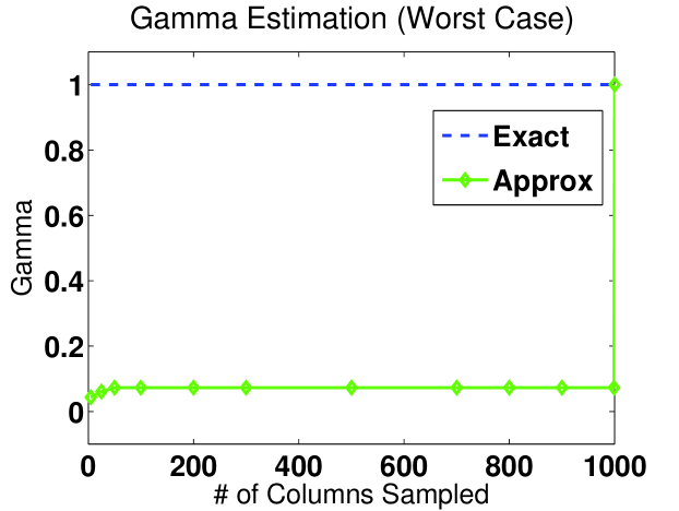
In spite of these discouraging worst-case results, our extensive empirical studies show that Estimate-Coherence performs quite well in practice on a variety of synthetic and real datasets with varying coherence, suggesting that the worst case addressed in theory and matched empirically in Figure 2 is rarely encountered in practice. We present these results in the remainder of this section.

(a)	(b)
(c)	(d)
(e)	(f)

Figure 3: Experiments with synthetic matrices. (a) True coherence associated with ‘low’, ‘mid’ and ‘high’ coherences. (b-d) Exact low-rank experiments measuring difference between the exact coherence and the estimate by Estimate-Coherence. (e-f) Experiments with low-rank matrices in the presence of noise, comparing exact and estimated coherence with two different levels of noise.

5.1 Experiments with synthetic data

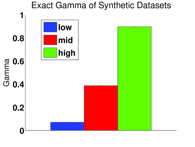
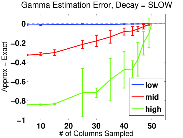
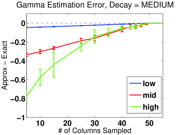
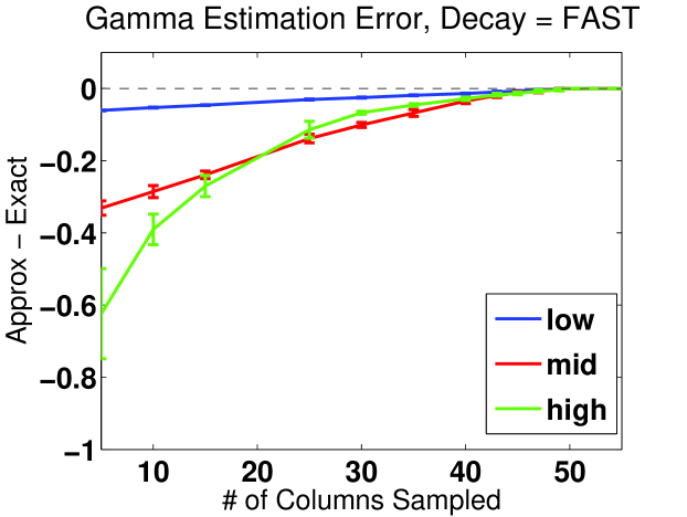
We first generated low-rank synthetic matrices with varying coherence and singular value spectra, with $n=m=1000$, and $r=50$. To control the low-rank structure of the matrix, we generated datasets with exponentially decaying eigenvalues with differing decay rates, i.e., for $i\in\{1,\ldots,r\}$ we defined the $i$th singular value as $\sigma_{i}=\exp(-i\eta)$, where $\eta$ controls the rate of decay and $\eta_{slow}=.01,\,\eta_{medium}=.1,\,\eta_{fast}=.5$. To control coherence, we independently generated left and right singular vectors with varying coherences by manually defining one singular vector and then using QR to generate $r-1$ additional orthogonal vectors. We associated this coherence-inducing singular vector with the $r/2$ largest singular value. We defined our ‘low’ coherence model by forcing the coherence-inducing singular vector to have minimal coherence, i.e., setting each component equal to $1/\sqrt{n}$. Using this as a baseline, we used $3$ and $8$ times this baseline to generate ’mid’ and ’high’ coherences (see Figure 3(a)). We then used Estimate-Coherence with varying numbers of sampled columns to estimate matrix coherence. Results reported in Figure 3(b-d) are means and standard deviations of $10$ trials for each value of $l$. Although the coherence estimate converges faster for the low coherence matrices, the results show that even in the high coherence matrices, Estimate-Coherence recovers the true coherence after sampling only $r$ columns. Further, we note that the singular value spectrum influences the quality of the estimate. This observation is due to the fact that the faster the singular values decay, the greater the impact of the $r/2$ largest singular value, which is associated with the coherence-inducing singular vector, and hence the more likely it will be captured by sampled columns.

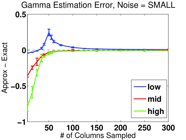
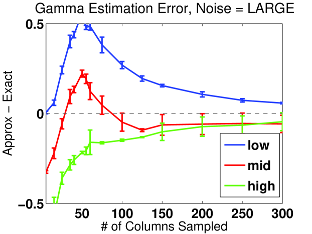
Next, we examined the scenario of low-rank matrices with noise, working with the ‘MEDIUM’ decaying matrices used in the low-rank experiments. To create a noisy matrix from each original low-rank matrix, we first used the QR algorithm to find a full orthogonal basis containing the $r$ left singular vectors of the original matrix, and used it as our new left singular vectors (we repeated this procedure to obtain right singular vectors). We then defined each of the remaining $n-r$ singular values of our noisy matrix to equal some fraction of the $r$th singular value of the original matrix ($0.1$ for ‘SMALL’ noise and $0.9$ ‘LARGE’ noise). The performance of Estimate-Coherence on these noisy matrices is presented in Figure 3(e-f), where results are means and standard deviations of $10$ trials for each value of $l$. The presence of noise clearly has a negative affect on performance, yet the estimates are quite accurate for $l=2r$ in the ‘LOW’ noise scenario, and even for the high coherence matrices with ‘LARGE’ noise, the estimate is fairly accurate when $l\geq 4r$.

5.2 Experiments with real data

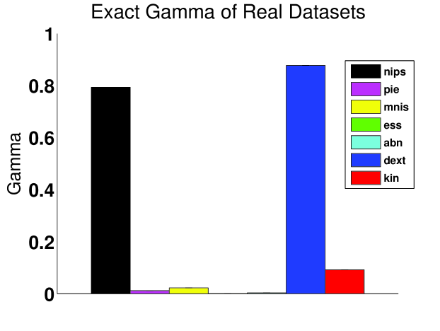
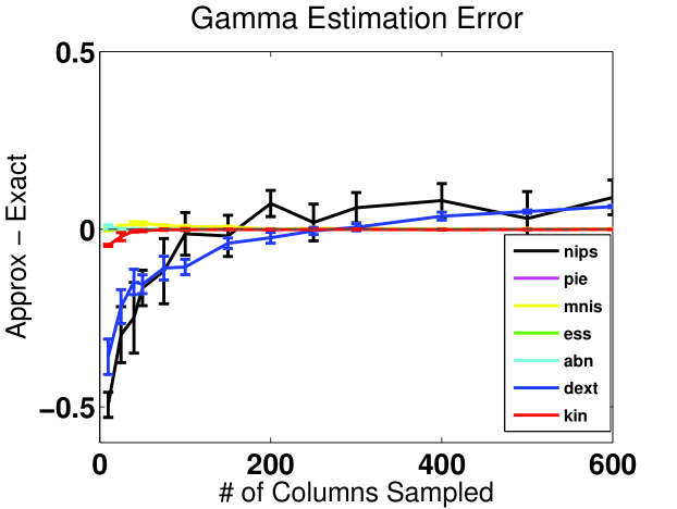
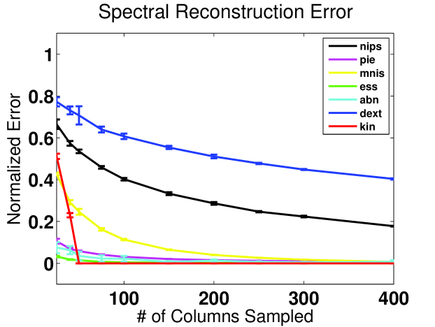
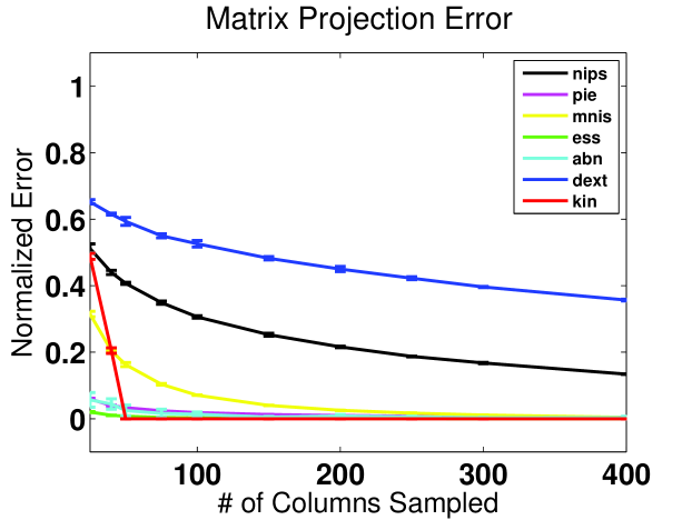
We next performed experiments using the datasets listed in Table 1. We used a variety of kernel functions to generate SPSD kernel matrices from these datasets, with the resulting kernel matrices being quite varied in coherence (see Figure 4(a)). We then used Estimate-Coherence with $r$ set to equal the number of singular values needed to capture $99\%$ of the spectral energy of each kernel matrix. Figure 4(b) shows the estimation error over $10$ trials. Although the coherence is well estimated across datasets when $l\geq 100$, the estimates for the two high coherence datasets (nips and dext) converge most slowly and exhibit the most variance across trials. Next, we performed spectral reconstruction using the Nyström method and matrix projection reconstruction using the Column-sampling method, and report results over $10$ trials in Figure 4(c-d). The results clearly illustrate the connection between matrix coherence and the quality of these low-rank approximation techniques, as the two high coherence datasets exhibit significantly worse performance than the remaining datasets.

Dataset	Type of data	# Points ($n$)	# Features ($d$)	Kernel
NIPS	bag of words	$1500$	$12419$	linear
PIE	face images	$2731$	$2304$	linear
MNIS	digit images	$4000$	$784$	linear
Essential	proteins	$4728$	$16$	RBF
Abalone	abalones	$4177$	$8$	RBF
Dexter	bag of words	$2000$	$20000$	linear
KIN-8nm	kinematics of robot arm	$2000$	$8$	polynomial

Table 1: Description of real datasets used in our coherence experiments, including the type of data, the number of points ($n$), the number of features ($d$) and the choice of kernel (Sim et al., , 2002; LeCun and Cortes, , 1998; Gustafson et al., , 2006; Asuncion and Newman, , 2007).

(a)	(b)
(c)	(d)

Figure 4: Experiments with real data. (a) True coherence of each kernel matrix ${\mathbf{K}}$. (b) Difference between the true coherence and the estimated coherence. (c-d) Quality of two types of low-rank matrix approximations ($\widetilde{\mathbf{K}}$), where ‘Normalized Error’ equals $\lVert{\mathbf{K}}-\widetilde{\mathbf{K}}\rVert_{F}/\lVert{\mathbf{K}}\rVert_{F}$.

6 Conclusion

We proposed a novel algorithm to estimate matrix coherence. Our theoretical analysis shows that Estimate-Coherence provides good estimates for relatively low-coherence matrices, and more generally, its effectiveness is tied to coherence itself. We corroborate this finding for high-coherence matrices with an adversarially chosen dataset and sampling scheme. Empirically, however, our algorithm efficiently and accurately estimates coherence across a wide range of datasets, and these estimates are excellent predictors of the effectiveness of sampling-based matrix approximation. We believe that our algorithm should be used whenever low-rank matrix approximation is being considered to determine its applicability on a case-by-case basis. Moreover, the variance of coherence estimates across multiple samples may provide further information, and the use of multiple samples fits nicely in the framework of ensemble methods for low-rank approximation, e.g., Kumar et al., (2009a).

References

- Asuncion and Newman, (2007) A. Asuncion and D.J. Newman. UCI machine learning repository. http://www.ics.uci.edu/~mlearn/MLRepository.html, 2007.
- Bach and Jordan, (2005) Francis R. Bach and Michael I. Jordan. Predictive low-rank decomposition for kernel methods. In International Conference on Machine Learning, 2005.
- Candès and Plan, (2009) Emmanuel J. Candès and Yaniv Plan. Matrix completion with noise. arXiv:0903.3131v1, 2009.
- Candès and Recht, (2009) Emmanuel J. Candès and Benjamin Recht. Exact matrix completion via convex optimization. Foundations of Computational Mathematics, 9(6):717–772, 2009.
- Candès and Romberg, (2007) E. J. Candès and J. Romberg. Sparsity and incoherence in compressive sampling. Inverse Problems, 23(3):969–986, 2007.
- Candès and Tao, (2009) Emmanuel J. Candès and Terence Tao. The power of convex relaxation: Near-optimal matrix completion. arXiv:0903.1476v1[cs.IT], 2009.
- Candès et al., (2006) Emmanuel J. Candès, Justin K. Romberg, and Terence Tao. Robust uncertainty principles: exact signal reconstruction from highly incomplete frequency information. IEEE Transactions on Information Theory, 52(2):489–509, 2006.
- Candès et al., (2009) Emmanuel J. Candès, Xiaodong Li, Yi Ma, and John Wright. Robust principal component analysis? arXiv:0912.3599v1[cs.IT], 2009.
- Deshpande et al., (2006) Amit Deshpande, Luis Rademacher, Santosh Vempala, and Grant Wang. Matrix approximation and projective clustering via volume sampling. In Symposium on Discrete Algorithms, 2006.
- Donoho, (2006) David L. Donoho. Compressed Sensing. IEEE Transactions on Information Theory, 52(4):1289–1306, 2006.
- Drineas and Mahoney, (2005) Petros Drineas and Michael W. Mahoney. On the Nyström method for approximating a Gram matrix for improved kernel-based learning. Journal of Machine Learning Research, 6:2153–2175, 2005.
- Drineas et al., (2006) Petros Drineas, Ravi Kannan, and Michael W. Mahoney. Fast Monte Carlo algorithms for matrices II: Computing a low-rank approximation to a matrix. SIAM Journal of Computing, 36(1), 2006.
- Fergus et al., (2009) Rob Fergus, Yair Weiss, and Antonio Torralba. Semi-supervised learning in gigantic image collections. In Neural Information Processing Systems, 2009.
- Fowlkes et al., (2004) Charless Fowlkes, Serge Belongie, Fan Chung, and Jitendra Malik. Spectral grouping using the Nyström method. Transactions on Pattern Analysis and Machine Intelligence, 26(2):214–225, 2004.
- Frieze et al., (1998) Alan Frieze, Ravi Kannan, and Santosh Vempala. Fast Monte-Carlo algorithms for finding low-rank approximations. In Foundation of Computer Science, 1998.
- Gustafson et al., (2006) A. Gustafson, E. Snitkin, S. Parker, C. DeLisi, and S. Kasif. Towards the identification of essential genes using targeted genome sequencing and comparative analysis. BMC:Genomics, 7:265, 2006.
- Keshavan et al., (2009a) Raghunandan Keshavan, Andrea Montanari, and Sewoong Oh. Matrix completion from noisy entries. In Neural Information Processing Systems, 2009.
- Keshavan et al., (2009b) Raghunandan Keshavan, Andrea Montanari, and Sewoong Oh. Matrix completion with a few entries. arXiv:0901.3150v4[cs.LG], 2009.
- Kumar et al., (2009a) Sanjiv Kumar, Mehryar Mohri, and Ameet Talwalkar. Ensemble Nyström method. In Neural Information Processing Systems, 2009.
- Kumar et al., (2009b) Sanjiv Kumar, Mehryar Mohri, and Ameet Talwalkar. On sampling-based approximate spectral decomposition. In International Conference on Machine Learning, 2009.
- LeCun and Cortes, (1998) Yann LeCun and Corinna Cortes. The MNIST database of handwritten digits. http://yann.lecun.com/exdb/mnist/, 1998.
- Sim et al., (2002) Terence Sim, Simon Baker, and Maan Bsat. The CMU pose, illumination, and expression database. In Conference on Automatic Face and Gesture Recognition, 2002.
- Smola and Schölkopf, (2000) Alex J. Smola and Bernhard Schölkopf. Sparse Greedy Matrix Approximation for machine learning. In International Conference on Machine Learning, 2000.
- Talwalkar and Rostamizadeh, (2010) Ameet Talwalkar and Afshin Rostamizadeh. Matrix coherence and the Nyström method. arXiv:1004.2008v1[cs.AI], 2010.
- Talwalkar et al., (2008) Ameet Talwalkar, Sanjiv Kumar, and Henry Rowley. Large-scale manifold learning. In Conference on Vision and Pattern Recognition, 2008.
- Williams and Seeger, (2000) Christopher K. I. Williams and Matthias Seeger. Using the Nyström method to speed up kernel machines. In Neural Information Processing Systems, 2000.