Gravitational Lensing Accuracy Testing 2010 (GREAT10) Challenge Handbook

Abstract

GRavitational lEnsing Accuracy Testing 2010 (GREAT10) isa public image analysis challenge aimed at the development of algorithms to analyze astronomical images. Specifically, the challenge is to measure varying image distortions in the presence of a variable convolution kernel, pixelization and noise. This is the second in a series of challenges set to the astronomy, computer science and statistics communities, providing a structured environment in which methods can be improved and tested in preparation for planned astronomical surveys. GREAT10 extends upon previous work by introducing variable fields into the challenge. The “Galaxy Challenge” involves the precise measurement of galaxy shape distortions, quantified locally by two parameters called shear, in the presence of a known convolution kernel. Crucially, the convolution kernel and the simulated gravitational lensing shape distortion both now vary as a function of position within the images, as is the case for real data. In addition, we introduce the “Star Challenge” that concerns the reconstruction of a variable convolution kernel, similar to that in a typical astronomical observation. This document details the GREAT10 Challenge for potential participants. Continually updated information is also available from www.greatchallenges.info.

, , , , , , , , , , , , , , , , , , , , , , , , , , , , , , , , ,
and

t1Supported by STFC Rolling Grant Number RA0888 and an RAS 2010 Fellowship.

t8Supported by the Zwicky Fellowship at ETH Zurich.

t2Supported by the European Research Council under the EC FP7 ERC Grant Number 240185.

t4Supported by STFC Advanced Fellowship #PP/E006450/1 and ERC Grant MIRG-CT-208994.

t6Supported by the European DUEL Research-Training Network (MRTN-CT-2006-036133).

t3Supported by a Royal Society University Research Fellowship and a European Research Council Starting grant.

t5Supported in part by the Swiss National Science Foundation (SNSF).

t7Supported by STFC Grant ST/H008543/1.

1 Introduction

The GRavitational lEnsing Accuracy Testing (GREAT) challenges are a series of simulations that provide an environment within which image analysis algorithms of importance for gravitational lensing cosmology can be developed. The central theme of GREAT10 is variability, the simulations contain spatially variable quantities, and the challenge is to reconstruct the properties of these variable fields to a high accuracy.

Gravitational lensing is the effect that light rays are deflected by gravity. Every galaxy image is distorted by this effect because of mass that is always present between the galaxy and the observer. For the majority of galaxies this distortion causes a small additional ellipticity called shear. Measuring the shear allows us to extract information on the nature of the intervening lensing mass and the expansion of the Universe [see Bartelmann and Schneider (2001) for a technical review], in particular, shear can be used to illuminate the nature of dark matter, dark energy and possible deviations from general relativity. However, to enable gravitational lensing data to find this information, the shear needs to be determined to a high degree of accuracy.

The GREAT challenges are designed to aid in the development of algorithms, that aim to measure the gravitational lensing shear, by evolving lensing image simulations in a controlled manner. The first of the GREAT challenges, GREAT08 [Bridle et al. (2009)], began with the zeroth-order problem of measuring a spatially constant shear in the presence of a spatially constant convolution kernel (or Point Spread Function, PSF, impulse response). GREAT08 was inspired by the Shear TEsting Programme [STEP1, Heymans et al. (2006); STEP2, Massey et al. (2007)], which was a suite of simulations created by the lensing community and analyzed internally. GREAT08 was set as a PASCAL challenge to both the astronomy and computer science communities, to encourage the development of interdisciplinary approaches to this image processing problem, and was successful on various levels [Bridle et al. (2009)]. A high accuracy was achieved under the majority of simulated conditions, and there was participation from outside the gravitational lensing and cosmology communities; indeed, the winner [Hosseini and Bethge (2009)] was not a cosmologist.

In GREAT10 both the shear and the PSF are spatially varying quantities. The shear varies naturally across astronomical images because of the large scale distribution of matter in the Universe. The PSF varies spatially in images because of atmospheric effects and telescope optics. The primary aim for participants in GREAT10 will be to reconstruct the correlation function, or power spectrum, of the shear variation in the presence of a known but varying convolution kernel.

GREAT10 is a PASCAL challenge, set by cosmologists to the astronomy, computer science and statistics communities. The challenge will be launched in late 2010 and will run for 9 months. Algorithms that are successful when applied to these simulations will help cosmologists to exploit the scientific potential of current and future imaging surveys. These surveys will generate petabytes of imaging information ideal for gravitational lensing, and will necessitate automated data analysis.

In this article we will introduce the GREAT10 simulations in Section 2 and go into some detail in Section 3. We will also outline the submission process, and procedures through which we will evaluate results in Section 4. In Section 5 we conclude by discussing the scope and context of the simulations in relation to real data. We include a number of Appendices that contain technical details. We summarize the simulation and challenge details of GREAT10 in Figure 1.

2 The simulations

In GREAT10 we will introduce variable fields into the shear estimation challenge. Both the shear and the PSF will vary across the images. In Figure 2 we show how GREAT10 is related to the process through which we go from images of galaxies and stars to cosmological parameter estimation. There are a number of steps in this process that we will discuss in detail in this section.

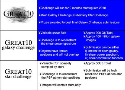
Figure 1: Top: A summary of the simulation and challenge details of GREAT10, which will consist of two separate but interconnected challenges, the main “Galaxy Challenge” and the “Star Challenge.”

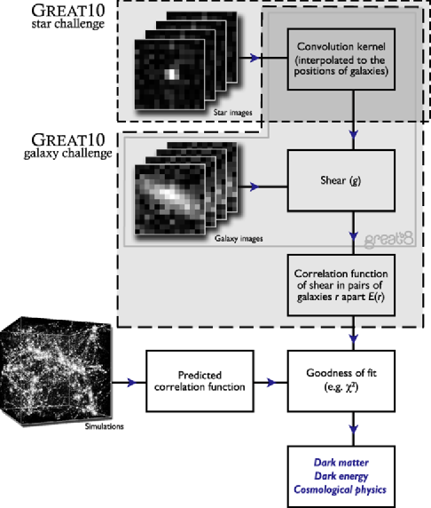
Figure 2: GREAT10 introduces two parallel challenges, both based on steps in the analysis of real astronomical data. The “Star Challenge” concerns the shapes of scattered stars. Each star is a local, noisy realization of the convolution kernel that is inevitably applied to any astronomical image (due to a combination of the Earth’s atmosphere, telescope optics and detector imperfections). This kernel varies smoothly across an image, and the challenge is to interpolate measurements between the locations of stars. The “Galaxy Challenge” concerns galaxy shapes, which must be measured after effectively deconvolving the image from a (supplied) model of the convolution kernel. This builds most closely on the previous GREAT08 challenge, but includes the crucial development that both the kernel and the distortion applied to the galaxy shapes now vary across an image. The required output is a measurement of the correlation between the shapes of pairs of galaxies separated by various distances. In a real cosmological analysis, the two procedures are applied in turn, then the correlations are compared to predictions of detailed simulations of the Universe.

To preface this section, we summarize the GREAT10 image simulation steps that represent each step of the lensing process:

• Undistorted Image: We start with an unsheared set of galaxies (with a distribution of ellipticities described in Appendix A) or point sources (stars).

• Shear Field Applied: The galaxy images, but not the star images, are transformed using a local distortion matrix that varies spatially across the image, a “shear” field.

• Convolution: Both the sheared galaxy images and star images are locally convolved by a Point Spread Function that varies spatially across the image.

• Pixelization: The convolved star and galaxy images are pixelized by summing the intensity in square pixels.

• Noise: Uncorrelated Gaussian distributed (homoskedastic) noise is added to all images. The image simulation process will also create Poisson noise.

Further details are given in Figures 1, 2 and 8. In this section we will describe the cosmologically important shear field and the type of convolution kernel that images experience.

2.1 Gravitational shear

As a photon propagates from a galaxy to an observer, the path that the light takes is distorted, or lensed, by the presence of mass along the line of sight. The first-order effect that this gravitational lensing has on the image of a galaxy is to introduce a local distortion that can be expressed as a remapping of the unlensed, original, pixels

$$\pmatrix{x_{\mathrm{original}}\cr y_{\mathrm{original}}}=\left[\pmatrix{1&0\cr 0&1}-|g|\pmatrix{\cos(2\phi)&\sin(2\phi)\cr\sin(2\phi)&-\cos(2\phi)}\right]\pmatrix{x_{\mathrm{observed}}\cr y_{\mathrm{observed}}},$$ (1)

where $x$ and $y$ denote a coordinate system that describes the observed light distribution of an object. The second term in this expression is known as the shear, and has the effect of stretching an object in a direction parameterized by an angle $\phi$ by an amount $|g|$.

It is important to note that the factor of $2$ in angle means that the shear is rotationally symmetric under rotations of $180$ degrees. In general, we define the shear as a local complex variable

$$g=|g|\mathrm{e}^{2\mathrm{i}\phi}=|g|[\cos(2\phi)+\sin(2\phi)]=g_{1}+\mathrm{i}g_{2},$$ (2)

where $g_{1}$ represents local “$+$ type” distortions (along the Cartesian axes) and $g_{2}$ represents local “$x$ type” distortions (along the $45$ degree axes). Equation (1) can now be rewritten in terms of $g_{1}$ and $g_{2}$ as

$$\pmatrix{x_{\mathrm{original}}\cr y_{\mathrm{original}}}=\pmatrix{1-g_{1}&-g_{2}\cr-g_{2}&1+g_{1}}\pmatrix{x_{\mathrm{observed}}\cr y_{\mathrm{observed}}}.$$ (3)

The amplitude and direction of the shear $g$ that an object experiences depends on the amount and nature of the lensing matter, rendering this quantity of great interest to the cosmological community.

The shear effect, to first order, produces an additional ellipticity in an object image; here we define the ellipticity of an object as $e=(1-r)(1+r)^{-1}\exp(2\mathrm{i}\psi)$, where $r$ is the ratio of the major to minor axes in the image, and $\psi$ is an angle of orientation. A significant characteristic of gravitational lensing is that galaxies in general, and in GREAT10, already have an “intrinsic” presheared ellipticity $e^{\mathrm{intrinsic}}$ such that the measured ellipticity per galaxy can be expressed as

$$e^{\mathrm{observed}}=\frac{e^{\mathrm{intrinsic}}+g}{1+g^{*}e^{\mathrm{intrinsic}}}\approx e^{\mathrm{intrinsic}}+g,$$ (4)

where the approximation is true for small shear $|g|\ll 1$; in GREAT08 and GREAT10 the shear has values of $|g|\lesssim 0.05$. One aspect of the challenge for gravitational lensing is that we cannot directly observe the unsheared images of the galaxies that we use in the analyses.

2.2 Variable shear fields

The shear we observe varies spatially as a function of position on the sky. This variation reflects the distribution of mass in the Universe, which forms a “cosmic web” of structures within which galaxies cluster on all scales through the influence of gravity. As we observe galaxies, at different positions and at different distances, through this cosmic web the light from each galaxy is deflected by a different amount by a different distribution of mass along the line of sight. The effect is that the shear induced on galaxy images is not constant across the sky but instead varies in a way that reflects the large scale, nonuniform, distribution of mass in the Universe. This lensing by large scale structure is known as cosmic shear. The measurement of cosmic shear has been one of the major goals of gravitational lensing and promises to become one of the most sensitive methods with which we will learn about dark energy and dark matter.

The shear field we observe is in fact a spin-2 field. This means that it is a scalar field described locally by $g_{1}$ and $g_{2}$ components that introduce $180$ degree invariant distortions [the “$2$” in “spin-2” refers to the factor of 2 in (1) and (2)]. In this case equation (2) acts as a local coordinate transformation for each galaxy where $g_{1}(\theta_{x},\theta_{y})$ and $g_{2}(\theta_{x},\theta_{y})$ are now variable fields as a function of position ($\theta_{x}$, $\theta_{y}$).

A general spin-2 field can be written as a sum of an E-mode component (curl-free) or gradient term, and a B-mode component (grad-free) or curl term; E and B are used in analogy to the electric and magnetic components of an electromagnetic field. The cosmological effect on the shear field is to introduce an E-mode signal and only negligible B-mode, which means that a tangential shear is induced around any region of excess density (see Figure 4).

In GREAT10 we will evaluate methods on their ability to reconstruct the E-mode variation only. In real observations the unsheared orientations of galaxies will in general produce an E- and B-mode in the variation of the observed ellipticities [equation (4)]. However, in GREAT10 the unsheared population of galaxies will have a pure B-mode ellipticity distribution. This B-mode is introduced to reduce “ellipticity noise terms” in the simulations, and means that the size of the simulations is significantly reduced; this B-mode will not contribute to the E-mode variation with which we will evaluate the results. The intrinsic (undistorted) shape of a galaxy is not observable, galaxies always have the additional lensing distortion. The uncertainty on our knowledge of the intrinsic ellipticity of a galaxy, which is commonly related to the intrinsic variance in the ellipticities of the population, is what is refered to as “ellipticity noise.” We present a technical discussion of this aspect of the simulations in Appendix A.

2.3 Measuring a variable shear field

The galaxies we observe act as discrete points at which the shear field is sampled. The amount of shear induced on the observed image of an individual object is small, typically $\lesssim$3% (a change in the major-to-minor axis ratio of $\sim$1.06) and so techniques have been developed to measure statistical features of the shear distribution from an ensemble of galaxies. The mean of the shear field $\langle g_{i}\rangle$ is zero when averaged over sufficiently large scales, however, the variance of the shear field is nonzero and contains cosmological information. We wish to calculate the variance of the shear field as a function of scale (small scale means in close proximity in an image); a large variance on small scales, for example, would signify a matter distribution with structures on those scales (see Figure 3).

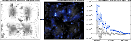
Figure 3: Real lensing effect on an ensemble of galaxy images. The shear distortion $g=g_{1}+\mathrm{i}g_{2}$ measured from the shapes of galaxies is represented in the left panel as a tick mark in the direction of $g$, with a length proportional to its magnitude. The amount of shear in a particular region of the image is determined by the amount of lensing material (dark matter) along the line of sight from the galaxy. Hence, we can reconstruct a map of the mass shown in the middle panel. We can also take the two-point correlation function of the shear field which is shown in the right panel. The left and middle panels show data from the Hubble COSMOS survey [Massey et al. (2007)] and the right panel shows a correlation function from the CFHT Legacy Survey [Fu et al. (2008)].

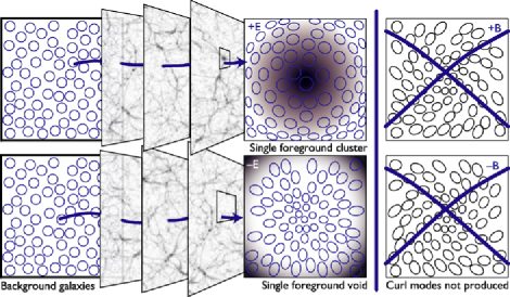
Figure 4: Schematic effect on an ensemble of galaxy images. The shear distortion varies as a function of position because the light propagates through the variable, foreground large scale structure (LSS) or “cosmic web.” The properties of the LSS imprint specific signatures on the type of distortion pattern. For example, if we had a sample of circular background galaxies (clear circles, left panels), they would be distorted into ellipses with major axes orientated tangent to density contours by a foreground mass overdensity, or radial shapes by a mass underdensity. These typically contribute to the cosmic shear on different physical scales, and their combined effect is an “E-mode” correlation function that varies as a function of scale. However, the LSS does not introduce significant “B-mode” or curl distortion patterns (represented by a cross X in this figure).

We can calculate the variance of the shear field as a function of scale by computing the two-point correlation function $\xi(\Delta\bolds\theta)$ of the shear field. The correlation function measures the tendency for galaxies at a chosen separation to have preferred shape alignment. For any given pair of galaxies we can define a component of the shear from each in terms of a tangential shear component, which is perpendicular to the line joining the pair, and a cross-component which is at $45$ degrees, this is meant to isolate the E- and B-mode signal shown in Figure 4. In Appendix B we show how to calculate the correlation function from galaxy shears.

Complementary to the correlation function is the power spectrum $C(\bolds\ell)$, which is simply the Fourier transform of the correlation function,

$$\xi(\Delta\bolds\theta) = \int C(\bolds\ell)\mathrm{e}^{\mathrm{i}\bolds\ell.\Delta\bolds\theta}\,\mathrm{d}^{2}\bolds\ell,$$

$$C(\bolds\ell) = \frac{1}{(2\pi)^{2}}\int\xi(\Delta\bolds\theta){\mathrm{e}}^{-{\mathrm{i}}\bolds\ell.\Delta\bolds\theta}\,\mathrm{d}^{2}\Delta\bolds\theta,$$

where $\bolds\ell=(\ell_{x}$, $\ell_{y})$ is a 2D wavevector probing scales of order $\Delta\bolds\theta=(2\pi)/|\bolds\ell|$. The shear power spectrum can again be related to the underlying matter distribution. In Appendix B we outline a simple method for creating the shear power spectrum from the local $g_{1}$ and $g_{2}$ shear estimators from each galaxy. When the simulations are made public we will also provide open-source code that will enable participants to create any of these statistics from a catalogue of discretely estimated shear values.

The reconstruction of the shear field variation to sufficient accuracy, in terms of the power spectrum or correlation function, is the GREAT10 Galaxy Challenge.

2.4 Simulating a variable shear field

In GREAT10 we will simulate the shear field as a Gaussian random field. These fields have a random distribution of phases, but a distribution of amplitudes described by the input power spectrum. These are simplified simulations relative to the real shear distribution. In particular, the filamentary structures seen in the “cosmic web” are due to more realistic effects, and will not be present in the GREAT10 simulations. In Figure 5 we show an example of the simulated shear field in a GREAT10 image.

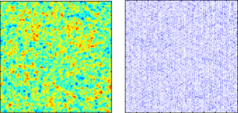
Figure 5: A GREAT10 simulated shear variation. An example of the variable shear field in a GREAT10 image. Left panel: we show the simulated mass distribution, which is a Gaussian realization with a particular power spectrum. Right panel: we show the shear represented by a line with length proportional to the amplitude of the shear $|g|$ and an angle $\phi$; see (1) and (2).

In addition to the cosmologically interesting shear effect, galaxy images are smoothed by a spatially variable convolution kernel (PSF).

2.5 Variable PSF

The images that we use in gravitational lensing analyses are smoothed and distorted by a convolution kernel (or Point Spread Function, PSF). The PSF that these images are convolved with is produced by a combination of effects:

• The images we use are created by observations with telescopes, which have a characteristic PSF that can vary as a function of position in the image due to the exact optical setup of the telescope and camera. Also, the detectors we use, Charge Coupled Devices (CCDs), pixelize the image; and defects can cause image degradation.

• When making observations with the telescopes on the ground the atmosphere acts to induce an additional PSF (due to refraction in the atmosphere and turbulence along the path of the photons).

• A telescope may move slightly during an observation, adding an additional smoothing component to the PSF. Typical observations last for seconds or minutes during which various effects (such as wind, temperature gradients, vibrations, etc.) can cause the telescope to move.

Each of these effects can vary across an image in either a deterministic fashion (as in telescope optics) or randomly (as in the atmosphere). In Figure 6 we show the effect on an ensemble of stars, both schematically and from realistic simulations. In Figure 7 we show the spatial variation of a simulated GREAT10 PSF.

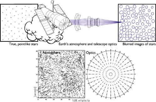
Figure 6: Upper panels: Schematic Effect of atmosphere and telescope optics. A distribution of point-like star images is blurred and the resulting pattern has variable spatial structure. Lower panels: Real Effect of the atmosphere [from Rowe (2010)] and telescope optics [example from Jarvis, Schechter and Jain (2008)] on the PSF ellipticity and size, respectively. The atmosphere adds random, coherent, patterns and the telescope adds specific functional behavior due to optical effects.

We can estimate the local PSF, in the presence of pixelization, from images of stars. This is because stars are point-like objects that only experience the convolving effect of the PSF and are not subject to the shear distortion; the stars we observe are part of our own galaxy, the Milky Way. The problem is that we have a discrete number of point-like PSF estimators in each image and a spatially varying PSF. What we need is an accurate PSF reconstruction at nonstar positions (the positions of the sheared galaxies).

There are currently two broad classes of approach that we define here that have been investigated to deal with this sparsely sample variable PSF:

• Direct modeling uses star images as discrete estimators of a spatially varying model (typically some low-order polynomial) and finds a best-fit solution to this model.

• Indirect modeling, for example, uses an ensemble of stellar images at different positions to extract principal components (or eigenvectors) of the PSF across the images.

These techniques, direct and indirect modeling, have been used on gravitational lensing images, but none have yet reached the required accuracy to fully exploit the most ambitious future gravitational lensing experiments.

In addition, there are a variety of deconvolution algorithims that attempt to remove the PSF from images by applying an algorithm that reverses the effect of the convolution. The deconvolution approach has been investigated, but has not been implemented with gravitational lensing observations to date. In Appendix E we outline in more detail these three PSF modeling approaches.

To first order the PSF is commonly parameterized with a size (usually defined using a Full-Width-Half-Maximum, FWHM, Gaussian measure) and an ellipticity, defined in a similar way to shear

$$e=|e|[\cos(2\psi)+\sin(2\psi)]=e_{1}+{\mathrm{i}}e_{2},$$ (6)

where again $e_{1}$ represents “$+$ type” distortions and $e_{2}$ represents “$x$ type” distortions. In the GREAT10 Galaxy Challenge the PSF will be provided as a known function $f(e,R)$ parameterized with a size $R(\theta_{x},\theta_{y})$ (FWHM) and ellipticity $e(\theta_{x},\theta_{y})$ that will vary across each image, so that any inaccuracies caused by PSF misestimation should be removed from the problem.

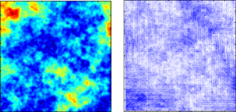
Figure 7: A GREAT10 simulated PSF variation. An example of the variable PSF field in a GREAT10 image. Left panel: we show the simulated magnitude of the ellipticity, which contains atmospheric and telescope optics effects. Right panel: we show the ellipcity represented by a line with length proportional to the amplitude of the ellipticity $|e|$ and an angle $\psi$; see (6).

However, in addition to measuring shear very accurately, PSF estimation is of crucial importance for gravitational lensing. If we cannot characterize the PSF sufficiently at galaxy positions, our shear values will be inaccurate. This is not addressed in the Galaxy Challenge where the PSF is a known function, so here we set the additional task of estimating the PSF at nonstar positions as a challenge in itself; the GREAT10 Star Challenge.

2.6 Summary of effects

To summarize the effects included in the simulations, we show the effect induced on an individual galaxy and star image in Figure 8. This “forward process,” from a galaxy to an image, was detailed in Bridle et al. (2009). Each galaxy image is distorted by the matter distribution, this image is then convolved by a PSF that spatially varies as a result of possible atmospheric effects and telescope optics, and finally the image is pixelized. Star images experience the convolution and pixelization but are not distorted by the shear field.

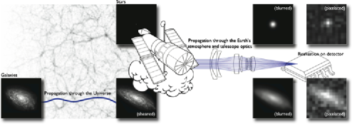
Figure 8: Summary of the main effects on an individual galaxy or star. This is the forward process described in Bridle et al. (2009), although GREAT10 includes additional realism in that both the induced gravitational shear distortion and the PSF vary as a function of position. The GREAT10 “Galaxy Challenge” is to estimate the shear distortion applied to a galaxy image, correcting for the additional effects in the Earth’s atmosphere and telescope optics, which are also experienced by the images of stars; for space-based telescopes the atmospheric effects are not present so that telescope and detector effects alone induce a PSF.

The GREAT08 challenge focused on the determination of the shear $g$, in the presence of these effects, by creating images in which a constant shear and a constant PSF had been applied to all objects (by creating constant-shear images, algorithms designed to estimate the average shear from an ensemble of galaxies can be tested). In GREAT10 we will move toward the more demanding, and more realistic, regime of variable shear fields.

In gravitational lensing analyses to date (c. 2010), we estimate the local shear from individual galaxies and use these to reconstruct the two-point statistics of the shear field. In Appendix D we review current methods that are used to estimate the shear from galaxies [including some advancements made since GREAT08; Bridle et al. (2009)].

3 Simulation details

In GREAT10 the main Galaxy Challenge is to reconstruct the shear field in the presence of a variable PSF. We also present the Star Challenge that is independent from the main challenge:

• Galaxy Challenge. This is the main challenge for GREAT10. The objective is to reconstruct the shear power spectrum. This is most similar to GREAT08. In this challenge the varying PSF will be a known function.

• Star Challenge. This separate challenge is to reconstruct the PSF at nonstar positions given an image of PSF convolved stars.

The GREAT10 structure is schematically represented in Figure 1.

3.1 Galaxy challenge

In each Galaxy Challenge image there will be a different realization of the shear power spectrum. The Galaxy Challenge will be subdivided into a low noise (high signal-to-noise) set and a realistic (real) noise set. The low noise subset will be closely matched in substructure to the real noise set such that participants will be able to analyze whether training on such data is of use in shape measurement. There will be fewer low noise images than real noise images (similar to GREAT08) to reflect our requirements on accuracy (see Section 4.2).

For the main Galaxy Challenge the input PSF will be provided as a functional form that will allow the spatially varying PSF to be reconstructed at any spatial position with sub-pixel resolution. Images will be supplied containing sheared galaxy images, and the approximate positions of each object will be provided. The participants will be asked to provide a reconstruction of the shear power spectrum at specified $\ell$ mode ($2\pi/\mbox{separation}$) values. Participants will submit either of the following:

• A “shear catalogue”: a value of $g_{1}$ and $g_{2}$ for every galaxy in each image.

• A correlation function as a function of separation: at the launch of the challenge we will specify the exact values and binning required for this type of submission.

• A shear power spectrum as a function of $\ell=2\pi/\mbox{separation}$: at the launch of the challenge we will specify the exact values and binning required for this type of submission.

In addition to the innovations of variable fields, we will also make the Galaxy Challenge simulation more realistic in that the distribution of galaxy properties, for example, size and signal-to-noise, will be continuous distributions rather than discrete in some images. The GREAT10 galaxy models are similar to those in GREAT08; they will consist of two components, a “bulge” and a “disk” (an exponential profile with ${\mathrm{e}}^{-kR^{1/n}}$ with $n=1$ and $n=4$, resp.); these components may be misaligned and have varying intensities.

3.2 Star challenge

In each Star Challenge image there will be a different PSF. These Star Challenge images will be grouped into sets that contain the same underlying PSF, except for the presence of a possible random component that will have a different realization in each image, to represent a series of gravitational lensing observations. The Star Challenge will only have one high signal-to-noise level. In real CCDs some bright stars can “saturate” the images and need to be masked, in GREAT10 there will be no saturated stars.

For the Star Challenge, participants will be asked to provide an estimation of the PSF at nonstar positions.

All additional necessary information on the simulations will be provided on the GREAT10 webpage at the time of launch. Participants will also be provided with training sets for each Challenge that will be exactly representative of some subset of the main Challenge—in real data we do not have training sets and would have to rely on simulations being accurate enough representations of the Universe, however, we invite participants to use the training data with the caveat that this may only guarantee unbiased results in some subset of the main Challenge.

4 The challenge

In this section we will summarize some of the practical details of the Challenge and define our evaluation procedure.

4.1 Challenge details

The GREAT10 competition will run for $9$ months. The competition will be to achieve the largest quality factors in either the Galaxy and Star Challenges. Each challenge will be run as a separate competition. We will award prizes for the largest average quality factor in the Galaxy Challenge (there will only be one prize for all types of submission: catalogue, power spectrum, correlation function). We will also award a prize, in either the Star or Galaxy Challenge, for a method that performs well under a variety of simulated conditions or whose innovation is particularly noteworthy. There will be a mid-challenge workshop and a final GREAT10 meeting, where we will present the Challenge prizes.

Participants will be required to download the simulation data. We will provide download nodes, hosted by GREAT10 team members, over various continents for ease of accessibility. The simulated data for GREAT10 will constitute approximately $900+50$ GB over the Galaxy and Star Challenges, respectively.

The submission process for the competition will be through a web interface similar to GREAT08 [Bridle et al. (2009); GREAT08 Handbook], with a live leaderboard of average quality factors continuously updated. We will also publish a detailed results paper where the performance of methods will be shown as a function of various properties of the simulated images. We outline some rules of the competition in Appendix F.

4.2 Challenge evaluation

Each submission will result in a shear power spectrum $C(\bolds\ell)$ being calculated, either directly by the participant or internally after a shear catalogue or correlation function submission. The submitted power spectrum will then be compared to the true input power spectrum for each image in the simulation and a quality factor calculated.

The quality factor for an individual image is defined using the difference between the submitted power spectrum and the input power spectrum [Amara and Réfrégier (2008)], which is related to variance of the measured and true shears. For image $i$ this is defined as

$$\sigma_{i}^{2}=\frac{1}{2\pi}\int_{\ell_{\min}}^{\ell_{\max}}\ell(\ell+1)|C^{\mathrm{input}}(\ell)-C^{\mathrm{submitted}}(\ell)|\,\mathrm{d}\ln\ell.$$ (7)

This is a quantity that has been used in cosmic shear analyses to gauge the impact of systematic effects on cosmological parameter constraints. The fact $\ell(\ell+1)$ comes from summing over density of states in Fourier space. For GREAT10 we define the Galaxy Challenge quality factor as

$$Q_{\mathrm{GREAT10}}\equiv\frac{\mathcal{N}}{\langle\sigma^{2}\rangle},$$ (8)

where the angular brackets denote an average over all images in the simulation. The numerator $\mathcal{N}$ will be determined subject to the exact range of scales $[{\ell_{\min}},{\ell_{\max}}]$ in (7), that will be defined at the challenge launch. The winner of the Galaxy Challenge will be the method that results in the largest average quality factor over all images. In the final analysis of the results we will also consider alternative measures such as the L-1 and L-2 norm of the shear estimates versus the true shears. The results of the Star Challenge will also be gauged by a quality factor, which we outline in Appendix E.

The GREAT10 quality factor is different from the GREAT08 factor [Bridle et al. (2009)], which used the root-mean-square of the shear residuals as the denominator. The GREAT08 quality factor, and goal, was designed primarily with an additive bias $\hat{g}=g+b$ in mind, as discussed in Bridle et al. (2009), $b$ in this case is a bias that is constant with respect to $g$. However, both STEP and GREAT08 have shown that multiplicative correction $\hat{g}=g\times f(g)$ is also important, where $f(g)$ can be some function of $g$ (possibly constant). The GREAT10 quality factor is sensitive to both these effects, as well as any misestimation of shear variance contributions ($\sigma^{2}_{g}$).

5 GREAT10 simplifications and future challenges

We expect GREAT10 to have a significant impact on the gravitational lensing and cosmological communities, enabling the exploitation of the next generation of experiments. The simulations we have designed present a unique challenge to computer science, statistics and astronomy communities; we require extreme accuracy from a very large data set, and have limited training data.

In GREAT10 we have set the challenge of estimating the variation of the gravitational lensing shear signal in the presence of a realistic PSF model. By advancing the GREAT challenges in this direction, we have addressed some of the simplified assumptions that were made in GREAT08. As a result, GREAT10 is a demanding challenge—however, this is only the second stage in a series of challenges that will work toward creating realistic gravitational lensing simulations. Some of the simplified assumptions in GREAT10 simulations compared to real data include the following:

• Gaussian Random Field: The shear distribution in GREAT10 is a Gaussian random field with random phases. In real data the field may have non-Gaussian signatures, and nonrandom phase information.

• Known PSF: With real data we must estimate the PSF and determine the shear from each image. In GREAT10 we have separated these problems into two challenges; in future GREAT challenges these aspects will be combined.

• Weak Lensing: The shear field in GREAT10 only contains galaxies that are weakly sheared (the local distortion entirely described by $g_{1}$ and $g_{2}$). In reality, second-order effects are present and galaxies can even be strongly distorted (into arcs) or multiply imaged.

• Simple Galaxy Shapes: The galaxies used in this Challenge are simple relative to real data (similar to GREAT08).

• Simple Noise Model: The noise in the GREAT10 images will contain a Poisson term from the image creation process, that mimic photon emission from galaxies and stars, and an additional Gaussian component, to mimic noise in detectors. In practice, there are unusable bad pixels which have to be flagged or removed.

• Background Estimation/Heteroskedasticity: The noise in GREAT10 is constant across the image, where the data is modeled as a signal plus additive noise. Real data will also have an uncertain additive background component whose estimation further complicates calculation of uncertainties.

• Image Construction: In GREAT10 objects are distributed across the image with no overlaps. Furthermore, each object will be classified to the participant as a star or galaxy. In reality, the identification of objects is a further problem, and objects commonly overlap.

• Masking: The GREAT10 images do not have any data missing. In reality, data can be missing or incomplete, for example, due to the layout of the CCDs used to create the images. Furthermore, areas of images in real data are intentionally masked, for example, around very bright stars (that saturate the images) and satellite tracks (that leave bright linear trails across images).

• Intrinsic Ellipticity: In GREAT10 the intrinsic (nonsheared) ellipticities have only B-mode correlation (see Appendix C). This is constructed to reduce the simulation size to a manageable level. In real data the unsheared galaxies are expected to have a random orientation (equal E- and B-mode). There are also secondary effects that act to align galaxies that are in close physical proximity which can contaminate the lensing signal.

We envisage that the next GREAT challenge will build upon GREAT10 by including one or more of these effects.

In addition, there are a multitude of further effects that will be present in real data, for example, nonlinear CCD responsivity and Charge Transfer Inefficiency (CTI), variation in exposure times across a data set and variation of the PSF as a function of wavelength, to name a few. A further challenge will be to handle the enormous amount of data, of order petabytes, that will need to be analyzed over reasonable timescales.

The ultimate challenge for methods developed and tested on the GREAT challenges will be their application to data. In partnership with state-of-the-art instrumentation, the GREAT challenges will help scientists use gravitational lensing to answer some of our most profound and fundamental questions about the Universe.

Appendix A Removal of intrinsic shape noise in variable shear simulations

In shear simulations we must make some effort to reduce the effect of the intrinsic ellipticity noise. This can be understood if we take an example requirement on the variance of shear systematics to be $\sigma^{2}_{\mathrm{sys}}=10^{-7}$, which is a requirement on the variance in the estimated shear values such that our cosmological parameter estimation is unbiased.

Assuming that the intrinsic (unsheared) ellipticities are independent and identically distributed random variables, with a variance $\sigma^{2}_{\varepsilon}$, we will need $N_{\mathrm{gal}}=(\sigma^{2}_{\varepsilon}/\sigma^{2}_{\mathrm{sys}})$ to reach this accuracy. If $\sigma^{2}_{\varepsilon}\sim 0.1$ (a typical empirically observed quantity), this means $N\sim 10^{6}$ galaxies are required per shear value to reach the systematic floor. In GREAT08, with $6\times 50$ shear values over $9$ simulation conditions, this results in a number which is large ($2.7\times 10^{8}$ galaxies) and difficult to analyze in a short timescale.

In constant shear simulations, as was done in GREAT08, galaxies can be created in pairs such that they have the same unsheared ellipticity except that one has been rotated by $90$ degrees. The $90$ degree rotation converts an ellipticity to $e\rightarrow-e$. If we have rotated (by 90 degrees) and unrotated galaxy pairs, then the intrinsic shape noise cancels to first order and the variance on the shear is reduced to $g^{2}(\sigma^{4}_{\varepsilon}/2N)$ [Massey et al. (2007)]. This can be understood if we write the shear estimator for a single object $i$ as

$$\tilde{g}^{i}_{\alpha}=e^{i}_{\alpha}+P^{i}g^{i}+{\mathcal{O}}(g^{2}),$$ (9)

where $P$ is some response factor (a matrix that partially encodes the effect of the PSF) and higher-order terms also encapsulate any noise. In a $90$ degree rotated image the shear estimator can be written as

$$\tilde{g}^{i}_{\alpha}=-e^{i}_{\alpha}+P^{i}g^{i}+{\mathcal{O}}(g^{2}).$$ (10)

It can be easily seen that by averaging the individual shear estimates the intrinsic ellipticity contribution cancels.

In variable shear simulations, like GREAT10, the $90$ degree rotation method cannot be used. In GREAT10 we require the E-mode correlation function or power spectrum to be reconstructed. If we have two images with $90$ degree rotated galaxies, then by taking the correlation of the above shear estimates equations (9) and (10) we have

$$\langle\tilde{g}_{\alpha}\tilde{g}_{\beta}\rangle_{\mathrm{unrot}} = \langle e_{\alpha}e_{\beta}\rangle+P^{2}\langle gg\rangle+{\mathcal{O}}(g^{4}),$$ (11)

$$\langle\tilde{g}_{\alpha}\tilde{g}_{\beta}\rangle_{\mathrm{rot}} = \langle e_{\alpha}e_{\beta}\rangle+P^{2}\langle gg\rangle+{\mathcal{O}}(g^{4}).$$ (12)

It can be seen from these that we cannot combine correlation function estimates from rotated and unrotated images to remove the intrinsic ellipticity correlation function, and preserving the shear correlation function. This is fundamentally because the intrinsic ellipticity correlation function is a random field, with equal E- and B-mode contributions.

For variable shear simulations we can take advantage of the fact that the shear correlation function contains E-mode correlations only. In GREAT10 the intrinsic ellipticity correlation function will contain B-mode correlations only. This means that the correlation function from any image can be written as in (11), where now $\langle e_{\alpha}e_{\beta}\rangle$ only contains B-mode correlation and $\langle gg\rangle$ only contains E-mode correlation. By taking the E-mode component of the shear estimate $\langle\tilde{g}\tilde{g}\rangle$, we will then eliminate any contribution from the intrinsic ellipticity distribution. Thus, the simulation size, like the $90$ degree-rotated case for constant shear images, will not be determined by the intrinsic ellipticity variance.

This step is unrealistic in that real galaxies are not expected to have any preferred unsheared correlation (to first order), but is necessary for public simulations to make the size of the challenge approachable.

Appendix B Calculating the shear correlation function and shear power spectrum for GREAT10

In this Appendix we present methods that can be used to estimate the shear correlation function and power spectrum from the individual shear estimators from each galaxy.

At the beginning of the challenge we will provide links to open-source code to calculate these various statistics, given a catalogue of shear values per galaxy. The Galaxy Challenge submission procedure will allow for either a shear catalogue (per galaxy), a correlation function or a power spectrum to be submitted.

Calculating the correlation function

Here we summarize Crittenden et al. (2002) (and reference to this article) where shear-correlation statistics are presented in detail.

If we define a Cartesian coordinate system ($\theta_{x}$, $\theta_{y}$) on a patch of sky (assumed small) and $\phi$ is the angle between the line joining two galaxies and the $x$-axis, then the tangential component can be written as $g_{+}=-[g_{1}\cos(2\phi)+g_{2}\sin(2\phi)]$ and the cross term as $g_{\times}=-[g_{1}\sin(2\phi)-g_{2}\cos(2\phi)]$. We can take the correlation function of these two quantities

$$\xi(\Delta\bolds\theta)_{+} = \langle g_{+}(\theta_{x},\theta_{y})g_{+}(\theta_{x},\theta_{y};\Delta\bolds\theta)\rangle,$$

$$\xi(\Delta\bolds\theta)_{\times} = \langle g_{\times}(\theta_{x},\theta_{y})g_{\times}(\theta_{x},\theta_{y};\Delta\bolds\theta)\rangle,$$

where $\Delta\bolds\theta$ is the average radial (angular) separation of galaxy pairs, and the angle brackets represent an average over all galaxy pairs within a considered $\theta$. Here we refer to sums over finite-width bins in $\theta$.

The E- and B-mode correlation functions are related to these observable correlations, combinations of $\xi_{+}(\Delta\bolds\theta)$ and $\xi_{-}(\Delta\bolds\theta)$, in the following way:

$$\xi_{E}(\Delta\bolds\theta) = \tfrac{1}{2}[\xi_{+}(\Delta\bolds\theta)+\xi_{\times}(\Delta\bolds\theta)]+\tfrac{1}{2}\nabla^{4}\chi^{-1}[\xi_{+}(\Delta\bolds\theta)+\xi_{\times}(\Delta\bolds\theta)],$$

$$\xi_{B}(\Delta\bolds\theta) = \tfrac{1}{2}[\xi_{+}(\Delta\bolds\theta)+\xi_{\times}(\Delta\bolds\theta)]-\tfrac{1}{2}\nabla^{4}\chi^{-1}[\xi_{+}(\Delta\bolds\theta)-\xi_{\times}(\Delta\bolds\theta)].$$

The operator $\nabla^{4}\chi^{-1}$ is most easily evaluated in Fourier space

$$\nabla^{4}\chi^{-1}g(r)=\int r^{\prime}{\mathrm{d}}r^{\prime}g(r^{\prime}){\mathcal{G}}(r,r^{\prime}),$$ (15)

where

$${\mathcal{G}}(r,r^{\prime})=\int\frac{k\,{\mathrm{d}}k}{2\pi}J_{0}(kr)J_{4}(kr^{\prime}).$$ (16)

See Crittenden et al. (2002) for more information. In Appendix E we define the correlation function in a complementary way in (32), where the binning in $\theta$ is more explicit.

Note that we expect the cosmological signal to contain nearly zero B-mode correlations (see Figure 4), but that in GREAT10 the B-modes reveal the intrinsic ellipticity distribution by design (see Appendix A). In GREAT10 the quality factor will be evaluated using the E-mode correlation only.

Calculating the power spectrum

Recall from (1) that we have two shear components and that these vary as a function of position across the fields $g_{1}(\theta_{x},\theta_{y})$ and $g_{2}(\theta_{x},\theta_{y})$. We can write the “shear” as a complex number such that

$$g=g_{1}+{\mathrm{i}}g_{2},$$ (17)

and we can Fourier transform the shear in the following way

$$g_{R}(\ell_{x},\ell_{y})+{\mathrm{i}}g_{I}(\ell_{x},\ell_{y})=\sum_{\mathrm{galaxies}}[g_{1}(\theta_{x},\theta_{y})+{\mathrm{i}}g_{2}(\theta_{x},\theta_{y})]{\mathrm{e}}^{-{\mathrm{i}}\bolds\ell.\bolds\theta},$$ (18)

where two new Fourier estimators have been created, a real and an imaginary part which are a function of $\ell=(\ell_{x}$, $\ell_{y})$. These are simply related to the original $g_{1}$ and $g_{2}$ by

$$g_{R}(\ell_{x},\ell_{y}) = \sum_{\mathrm{galaxies}}g_{1}(\theta_{x},\theta_{y})\cos(\ell_{x}\theta_{x}+\ell_{y}\theta_{y})$$

$${}+g_{2}(\theta_{x},\theta_{y})\sin(\ell_{x}\theta_{x}+\ell_{y}\theta_{y}),$$

$$g_{I}(\ell_{x},\ell_{y}) = \sum_{\mathrm{galaxies}}g_{2}(\theta_{x},\theta_{y})\cos(\ell_{x}\theta_{x}+\ell_{y}\theta_{y})$$

$${}-g_{1}(\theta_{x},\theta_{y})\sin(\ell_{x}\theta_{x}+\ell_{y}\theta_{y}).$$

We now have two estimators that are a function of $\ell_{x}$ and $\ell_{y}$, with each point in the ($\ell_{x}$, $\ell_{y}$) plane being a sum over all galaxies.

In cosmology we wish to decompose the shear field into an E- and a B-mode; cosmological structures should only create an E-mode signal. To make this decomposition, we can describe the ($\ell_{x}$, $\ell_{y}$) by an angle $\phi_{\ell}=\tan^{-1}(\ell_{y}/\ell_{x})$ and a scalar $\ell=\sqrt{\ell_{x}^{2}+\ell_{y}^{2}}$. The E- and B-mode fields can now be written as a simple rotation of the Fourier plane

$$E(\ell_{x},\ell_{y})+{\mathrm{i}}B(\ell_{x},\ell_{y}) = [\cos(2\phi_{\ell})-{\mathrm{i}}\sin(2\phi_{\ell})]$$

$${}\times[g_{R}(\ell_{x},\ell_{y})+{\mathrm{i}}g_{I}(\ell_{x},\ell_{y})],$$

$$E(\ell_{x},\ell_{y}) = \cos(2\phi_{\ell})g_{R}(\ell_{x},\ell_{y})+\sin(2\phi_{\ell})g_{I}(\ell_{x},\ell_{y}),$$

$$B(\ell_{x},\ell_{y}) = \cos(2\phi_{\ell})g_{I}(\ell_{x},\ell_{y})-\sin(2\phi_{\ell})g_{R}(\ell_{x},\ell_{y}).$$

Finally, the shear power spectrum can be defined as the modulus of the E-mode field

$$C(\ell)=\frac{|E(\ell_{x},\ell_{y})|^{2}}{2\pi},$$ (21)

where in practice the $C(\ell)$ is the average over some bin in $|\ell|$.

For data that is distributed as a grid in $\theta_{x}$ and $\theta_{y}$, the above calculations can be simplified even further written as a series of FFTs:

• Make a 2D FFT of the shear field $g(\theta_{x},\theta_{y})\rightarrow\mathcal{G}(\ell_{x},\ell_{y})$.

• Construct a 2D $\ell$-matrix $\bolds\ell=(2\pi/\theta_{x})+{\mathrm{i}}(2\pi/\theta_{y})$.

• Rotate the FFT of the shear field $\mathcal{G}^{R}(\ell_{x},\ell_{y})\rightarrow(\bolds\ell^{*}\bolds\ell^{*}/|\bolds\ell^{2}|)\mathcal{G}(\ell_{x},\ell_{y})$.

• Inverse FFT the rotated shear field back to real space $\mathcal{G}^{R}(\ell_{x},\ell_{y})\rightarrow E(\theta_{x},\allowbreak\theta_{y})+{\mathrm{i}}B(\theta_{x},\theta_{y})$.

• Select the real part, E-mode and FFT $E(\theta_{x},\theta_{y})\rightarrow\mathcal{E}(\ell_{x},\ell_{y})$ (which is now complex).

• Calculate the modulus $|\mathcal{E}(\ell_{x},\ell_{y})|^{2}=\mathrm{Re}[\mathcal{E}(\ell_{x},\ell_{y})^{2}]+\operatorname{Im}[\mathcal{E}(\ell_{x},\ell_{y})^{2}]$ and azimuthally bin in $|\bolds\ell|$ to find the power spectrum.

At the launch of GREAT10 we will specify exactly which binning scheme in $\ell_{x}$, $\ell_{y}$ and $\ell$ we will use to calculate the result, and we will also specify the angular binning $\theta$ we require for correlation function submissions.

Note that the method described in this section will not work in the case that images are masked. In Section 5 we describe how masking is present in real data and may be included in future GREAT challenges.

Appendix C Overview of existing shape measurement methods

We refer the reader to the GREAT08 articles, Bridle et al. (2009), for a comprehensive review of shape measurement methods up until late 2009. Since the publication of the GREAT08 results paper and up until the creation of this Handbook, mid-2010, there have been several ongoing activities in the field.

The GREAT08 simulation details have been made public, both shear values (answers) for the simulations have been made available and the properties of each individual object in the simulations (these can be found by following the relevant links from http://www.greatchallenges.info).

In the interim period a new blind realization of GREAT08 has been released, GREAT08reloaded. This simulation is exactly the same as GREAT08 except that the true shears (answers) have new values. These simulations can be used as a semi-blind challenge such that developing algorithms can be tested on new simulated data. A new online quality factor calculator is available, but we do not show an online ranking at http://www.greatchallenges. info. Authors of newly developed algorithms are encouraged to publish new quality factor results from these simulations (please inform T. Kitching and S. Bridle if you intend to publish results based on GREAT08reloaded).

Some new methods have been published in this interim period. Bernstein (2010) has presented an investigation into several effects, related to model fitting algorithms, that impact shear measurement biases. Zhang (2010) has investigated mapping from ellipticity to shear and has presented a number of shear estimators with varying success. Gruen et al. (2010) have used a neural net approach, similar to those used for estimating galaxy distances (redshifts), to estimate shear. Melchior et al. (2010) have introduced a model-independent deconvolution method. Two of these new approaches, Bernstein (2010) and Gruen et al. (2010), have claimed significantly improved GREAT08 quality factors of $Q_{\mathrm{GREAT08}}\gtrsim 1\mbox{,}000$ on the low-noise subsets, and Melchior et al. (2010) have claimed $Q_{\mathrm{GREAT08}}\gtrsim 500$ on some real-noise subsets.

Appendix D Overview of existing PSF modeling methods

In this Appendix we will describe the techniques currently used by the gravitational lensing community to characterize the spatial variation of the PSF. We classify these approaches under three broad headings, as discussed in Section 2.5.

Direct modeling

The modeling of the spatial variation of the PSF across an image can take the form of fitting simple, continuous surfaces to quantities that parametrize the PSF at a given location. In this case a surface is fit to the image and the best fit is found by determining an extreme value of some goodness of fit, usually a minimum chi-square, calculated discretely at the star positions. The quantity being fit can either be the pixel intensities themselves or some derived quantity such as the ellipticity and Full-Width-Half-Maximum (FWHM) of the stars.

For example, in the KSB shear measurement method (see the GREAT08 Handbook Appendix B) these are usually the two components of the stellar anisotropy correction, estimated using the measured ellipticities of stars. Another method is to model PSFs using shapelet basis functions [e.g., Bernstein and Jarvis (2002); Refregier (2003); Massey and Refregier (2005); Kuijken (2006); Bergé et al. (2008)], where at each star a shapelet model is fit and it is the spatial variation in each shapelet coefficient that describes the PSF surface. In lensfit [Miller et al. (2007); Kitching et al. (2008)] implementations to date, the PSF is modeled on a pixel-by-pixel basis where for each pixel in a postage stamp a 2D polynomial is fit across the image. PSFEx [e.g., Kalirai et al. (2003)] combines several model fitting aspects, allowing for various different orthonormal expansions in 2D to be used. Regardless of the PSF model parameter being modeled, there is considerable freedom in the choice of the functional form of the fitting surface [see, however, Rhodes et al. (2007) and Jarvis, Schechter and Jain (2008) for attempts to use PSF models motivated by realistic optical patterns]; however, simple bivariate polynomials are typically used.

There are well-known problems with polynomial fitting surfaces, including reduced stability at field edges and corners, as the fits become poorly constrained. These have been noted but not necessarily tackled beyond suggestions of other, perhaps better behaved, functional schemes [e.g., Van Waerbeke, Mellier and Hoekstra (2005)]. Alternatively, it has been suggested [e.g., Kuijken (2006)] that the images can be Gaussianized to create a better behaved local functional variation of the PSF, at expense of correlated noise properties, however, global PSF interpolation is still required for such processes.

Indirect modeling: Principal component analysis (PCA)

Indirect modeling applies to a class of methods that do not model the PSF explicitly, for example, using some kind of polynomial, but attempt to characterize the variation across the image by finding patterns that are present between many realizations of the same underlying PSF. Principal Component Analyses (PCA; also known as eigenfunction analyses) are an example of this kind of PSF modeling that has been implemented by the community.

The motivation for such techniques is that gravitational lensing images (especially at particular positions, for example, away from the plane of the Milky Way) often contain only $\lesssim$1 star/arcmin² usable for PSF measurements. If the PSF shows spatial variations on this or smaller scales, they cannot be modeled reliably using a standard direct modeling interpolation, for example, with polynomial functions. However, these small-scale variations may show some degree of stability between different images (exposures) obtained using the same instrument, depending on their physical origin. If this is the case, one can attempt to combine the information from different exposures—with stars at different pixel positions—to obtain a PSF model with improved spatial interpolation.

A PCA interpolation was suggested for use in gravitational lensing by Jarvis and Jain (2004). They used PCA to identify the main directions of PSF variation between their exposures. This is typically done by first computing a standard polynomial interpolation in each exposure, where the polynomial order should be chosen to be sufficiently low to avoid overfitting. The PCA is then run on these polynomial coefficients. In this way the recurring PSF patterns in the different exposures can be described as a superposition of principal component patterns, where each exposure is characterized by its principal component coefficients. These coefficients yield a sorting scheme which enables the desired combination of stars from different exposures.

As the final step the stars from all exposures are fit together with a high-resolution model. In the description of Jarvis and Jain (2004) this model contains one higher-order spatial polynomial for each principal component. For the stars of a certain exposure these different polynomial terms are weighted according to the principal component coefficients of this exposure. Besides the polynomial order, one has to choose the number of included principal components. The first principal component is the most important one, carrying the largest variation in PSF space. The higher principal components carry less and less variation, and may at some point be truncated to avoid the fitting of noise, for example, once 99% of the variation are taken into account.

Some of the principal components (eigenfunctions) can have a physical interpretation, for example, in relation to the telescope optics (see Section 2.5). The principal components of the PSF are expected to have some relation to the main physical effects influencing the PSF, such as changes in telescope focus, seeing, wind-shake or pointing elevation. However, in detail, the cross-identification may be difficult, in particular, for the higher, less important principal components.

The PCA approach does not capture PSF variations which are completely random and appear in a single exposure only. On large scales these can be accounted for by combining the PCA model with a low-order residual polynomial fit, computed separately for each exposure [see Appendix B.5 of Schrabback et al. (2010)]. However, on small scales such random variations cannot be corrected.

Also, given that PCA is a linear coordinate transformation, it does not efficiently describe possible nonlinear distributions of exposures in the PSF coefficient space. Such nonlinear distributions may, in particular, occur if PSF quantities with different responses to physical parameters are fitted together. For example, telescope defocus changes PSF ellipticity linearly, whereas PSF size is affected quadratically. If one aims at a compact PSF description with few principal components, this can partially be compensated using additional terms in the final PCA fitting step, which depend nonlinearly on the principal component coefficients [see Schrabback et al. (2010)].

Image deconvolution

Astronomical images can be blurred for various reasons: for example, atmospheric turbulence for ground-based telescopes, or thermal deformations of the telescope through varying exposure to sunlight for space-based telescopes. Methods for deconvolution and deblurring can often alleviate those effects [e.g., Kundur and Hatzinakos (1996) and references therein]. There are three aspects of the deconvolution process that we comment on here:

• Nonblind vs. blind. In astronomy the point spread function (PSF), which describes the blur, can often be estimated from nearby stars, allowing nonblind deconvolution to deblur recorded images (called nonblind because the PSF is known). However, the PSF might not be available or cannot be reliably guessed. In that case blind methods try to recover simultaneously the PSF and the underlying image. This is usually achieved by optimization with alternating projections in combination with prior assumptions about the PSF and the image.

• Single-frame vs. multi-frame. Especially important for nonastronomical photography is single-frame deconvolution, in which we only observe a single blurry image and would like to recover a deblurred image [e.g., Fergus et al. (2006) and Cho and Lee (2009)]. In astronomy we are often able to record multiple images of the same object. Combining a large number of frames can then recover a single deblurred frame [e.g., by speckle-interferometric methods such as Labeyrie (1970); Knox and Thompson (1974), or by multi-frame deconvolution methods, e.g., Schulz (1993); Harmeling et al. (2009)].

• Space-invariant vs. space-variant. A common assumption is that the PSF is space-invariant, that is, in different parts of the image, the blur of a single star looks the same. For atmospheric turbulence this assumption holds only inside the isoplanatic patch, which is a small angular region the size of which depends on the amount of air turbulence. For images of larger angular regions (beyond the isoplanatic patch), the PSF does change across the image and this must be taken into account. Common approaches chop the image into overlapping patches with constant PSF and interpolate between them [e.g., Nagy and O’Leary (1998); Bardsley et al. (2006); Hirsch et al. (2010)].

Finally, we note that in astronomical images the presence of significant noise (typical objects used for cosmic shear have signal-to-noise ratios of $\approx$10–$20$) is a challenge to deconvolution algorithms.

Other methods

While the direct and indirect modeling methods described so far in this Appendix have been fully tested and applied to real data, there are other techniques that have been proposed as potentially useful for modeling the spatial variation in the PSF. We now discuss two of these suggestions in brief.

Kernel Principal Component Analysis [KPCA: e.g., Schölkopf, Smola and Müller (1998); Shawe-Taylor and Cristianini (2004)], a highly successful tool in pattern recognition, has been suggested as a further aid to stable PSF modeling. Variation in even basic aspects of a PSF (overall size, ellipticity, orientation) may often be difficult to succinctly describe in terms of linear combinations of image pixel values. This means that PCA models may sometimes require unnecessary degrees of freedom, which impacts upon the stability of accurate shear measurement. KPCA allows the Principal Components to be separated in a higher-dimensional feature space, mapped implicitly via a dot-product kernel, where these nonlinear dependencies can be unraveled.

Another statistical tool that might prove useful in spatial modeling of the PSF is known as kriging, commonly employed in the field of Geostatistics [see, e.g., Cressie (1991)]. This technique uses a weighted average of neighboring samples (in this case stars) to estimate the value of an unknown function at a given location. Weights are optimized using the location of the samples and all the relevant interrelationships between known and unknown values. The technique also quantifies confidence in model values. However, the accuracy of the method relies critically upon assumptions about the nature of the underlying variation; commonly-used types of kriging (such as Ordinary, Universal and IRFk-kriging) reflect the impact of differing choices for these assumptions. A further complication is the limited work done toward the application of kriging in the presence of noisy sampled data.

Appendix E Star challenge quality factors

The estimation of the PSF in images has a broad range of applications in astronomy beyond gravitational lensing, hence, we will define a quality factor that is flexible enough to allow nonlensing applications to gain useful information.

Each participant will submit a high resolution estimate of the PSF at each nonstar position that is requested. The quality factor that we will use to estimate the success of a method at estimating the PSF will calculate the residual (true PSF minus submitted estimate) for each nonstar position for each pixel. For astronomical analyses we are concerned with two basic parameters that have the highest impact on shape of the PSF: these are the ellipticity $e$ of the PSF and the size $R$ of the PSF [Paulin-Henriksson et al. (2008)]. These are defined as follows [see Bartelmann and Schneider (2001), Section 4.2].

First we define the second-order brightness moments of the image as

$$q_{ij}=\frac{\sum_{p}w_{p}I_{p}(\theta_{i}-\bar{\theta}_{i})(\theta_{j}-\bar{\theta}_{j})}{\sum_{p}w_{p}I_{p}},\qquad i,j\in\{1,2\},$$ (22)

where the sums are over pixels, $I_{p}$ is the flux in the $p$th pixel and $\theta$ is a pixel position ($\theta_{1}=x_{p}$ and $\theta_{2}=y_{p}$). We include a weight function $w_{p}$, that will be defined when the simulations are launched, to ensure that the sums over pixels converge for the exact PSF model used. We now write the weighted ellipticity for a PSF in complex notation as

$$e_{\mathrm{PSF}}=\frac{q_{11}^{2}-q_{22}^{2}+2{\mathrm{i}}q_{12}}{q_{11}^{2}+q_{22}^{2}+2(q_{11}q_{22}-q^{2}_{12})^{1/2}},$$ (23)

where we have used a definition of ellipticity $|e|=(1-r)(1+r)^{-1}$ which is consistent with Section 2; note there is an equivalent expression for $|e|=(1-r^{2})(1+r^{2})^{-1}$ [see Bartelmann and Schneider (2001), Section 4.2]. For the weighted size we have a similar expression

$$R_{\mathrm{PSF}}^{2}=q_{11}+q_{22}.$$ (24)

We can calculate the variance between the ellipticity of the model and true PSF $\sigma^{2}(e_{\mathrm{PSF}})\equiv\langle(e_{\mathrm{PSF}}-e_{\mathrm{PSF}}^{\mathrm{t}})^{2}\rangle$ and similarly for the size $\sigma^{2}(R_{\mathrm{PSF}})\equiv\langle(R_{\mathrm{PSF}}-R_{\mathrm{PSF}}^{\mathrm{t}})^{2}\rangle$.

For cosmic shear studies we have the requirement that we need the residual error in the ellipticity and size to be $\lesssim$10^-3 for the impact on cosmological parameter estimation to be low; for more detail see Paulin-Henriksson et al. (2008), Paulin-Henriksson, Refregier and Amara (2009). Hence, we define the quality factor for the Star Challenge as

$$P\equiv\frac{1}{({1/2})\langle\sigma^{2}(R_{\mathrm{PSF}})/R^{2}+\sigma^{2}(e_{\mathrm{PSF}})\rangle},$$ (25)

where the angle brackets represent an average over all images. There are further steps that could be taken that can map PSF residuals onto cosmic shear requirements [and indeed the Galaxy Challenge $Q$ factor; Paulin-Henriksson et al. (2008)]; we will present these in the final GREAT10 analysis.

In the following sections we outline more details on some additional PSF quality factors that we will employ in the final analysis. As well as the summed residual between the model and the data, we will investigate at least two other approaches that are more closely matched to the gravitational lensing requirements (but are less applicable to other fields of astronomy).

These techniques will not be used to determine the outcome of the competition or used to create live quality factors during the challenge.

Azithumal statistics

We can quantify the quality of the submitted PSF model in terms of how well a galaxy shear is recovered if this model were used. To do this, we will convolve the true PSF with a simple galaxy model, and then use the submitted PSF to recover the galaxy parameters from the true PSF-convolved image. This can be done for several angles in an azimuthal bin (ring) (and be repeated for zero shear and nonzero shear) to obtain multiplicative and additive errors on the measured shear [$m$ and $c$; see the Shear TEsting Programme; Heymans et al. (2006); Massey et al. (2007)]. These $m$, $c$ values can be converted into a GREAT08 $Q$ value (assuming a constant local shear). By comparing this ring test with the summed residuals, we will be able to correlate the magnitude of the residuals to the bias on the shear (i.e., $Q$).

Autocorrelations in residuals

The autocorrelation of any continuous function $h$ across its $n$-dimensional domain can be defined as

$$[h\star h](\mathbf{r})\equiv\int h^{*}(\mathbf{x})h(\mathbf{x}+\mathbf{r})\,\mathrm{d}^{n}x.$$ (26)

We may also employ the function $h(\mathbf{x})$ to represent a discrete, noisy sampling of an unknown “true” field $h_{\mathrm{t}}(\mathbf{x})$ such that

$$h(\mathbf{x})=h_{\mathrm{t}}(\mathbf{x})+N(\mathbf{x}),$$ (27)

where $N$ is a stochastic noise term. This description of discrete observations by a continuous “quasi-field” is a convenient notational shorthand in what follows; one can imagine the observations as a smooth field convolved with delta functions at the data locations. The data represented by $h(\mathbf{x})$ can be pixel values, complex ellipticities or any general data vector. Similarly, a best-fitting model used to characterize these observations can be written as

$$h_{\mathrm{m}}(\mathbf{x})=h_{\mathrm{t}}(\mathbf{x})+m(\mathbf{x},h_{\mathrm{t}},N;f_{\mathrm{m}}),$$ (28)

where the $m=h-h_{\mathrm{t}}$ is referred to as the inaccuracy in the model [Rowe (2010)] and $f_{\mathrm{m}}$ labels the specific modeling scheme chosen to represent $h(\mathbf{x})$.

The unknown function $m$ will depend nontrivially upon the data, noise and modeling scheme used, but not all of its properties are entirely hidden. If we make two simple assumptions about the noise in the data being considered, that

$$[N\star N](\mathbf{r})=0$$ (29)

and

$$[h_{\mathrm{t}}\star N+N\star h_{\mathrm{t}}](\mathbf{r})=0,$$ (30)

it follows that

$$[(h-h_{\mathrm{m}})\star(h-h_{\mathrm{m}})](\mathbf{r})=[m\star m](\mathbf{r})-[m\star N+N\star m](\mathbf{r}).$$ (31)

As demonstrated in Rowe (2010), this residual autocorrelation function should tend to zero for all $\mathbf{r}$ if the fitting model employed is both stable and accurate: the residuals are then indistinguishable from pure white noise. Departures from this ideal behavior have predictable consequences: overfitting models will show consistently negative values of $(h-h_{\mathrm{m}})\star(h-h_{\mathrm{m}})$ (since $[m\star N+N\star m]>m\star m>0$ in these cases), whereas underfitting models (for which $m\star m$ dominates) may be positive or negative in general.

If we consider the data in question to be an array of image pixels $I_{i}(\bolds\theta_{i})$, with a corresponding best-fitting model $I_{\mathrm{m}}$, we can construct a practical estimator $\hat{\xi}_{I}$ for the autocorrelation function in (31). We do this only in the isotropic case $\hat{\xi}_{I}(\theta)=\hat{\xi}_{I}(\bolds\theta)$ for simplicity, but note that the autocorrelation may not be isotropic in general.

Following Schneider et al. (2002), we estimate the correlation function in bins of finite width $\Delta\theta$ and define the function $\Delta_{\theta}(\phi)=1$ for $\theta-\Delta\theta/2<\phi<\theta+\Delta{\theta}/2$ and zero otherwise: thus, $\Delta_{\theta}(\phi)$ defines the bin at separation $\theta$. A simple estimator $\hat{\xi}_{I}$ for $(I-I_{\mathrm{m}})\star(I-I_{\mathrm{m}})$ may then be written as

$$\hat{\xi}_{I}(\theta)=\frac{1}{N_{\mathrm{p}}(\theta)}\sum_{ij}w_{i}w_{j}[I_{i}(\bolds\theta_{i})-I_{\mathrm{m}}(\bolds\theta_{i})][I_{j}(\bolds\theta_{j})-I_{\mathrm{m}}(\bolds\theta_{j})]\Delta_{\theta}(|\bolds\theta_{i}-\bolds\theta_{j}|),$$ (32)

where the sum is over all pixel pairs, the weight $w_{i}$ assigned to the $i$th pixel may be used to account for variations in the signal-to-noise across the image plane, and $N_{\mathrm{p}}(\theta)=\sum_{ij}w_{i}w_{j}\Delta_{\theta}(|\bolds\theta_{i}-\bolds\theta_{j}|)$ is the effective number of pairs in the bin considered.

Appendix F Rules of the challenge

The challenge will be run as a competition, and the winner will be awarded with a prize.

We will award a prize to the participants with the highest quality factor in the Galaxy Challenge at the end of the submission period. Prizes will be awarded at a final GREAT10 meeting, and winners will be required to make a descriptive presentation of their method at this workshop.

To define the scope of the competition we outline some participant rules here:

[(1)]

Participants may use a pseudonym or team name on the results leader board, however, real names (as used in publications) must be provided where requested during the result submission process. We will also require an email address to be provided, so that we can communicate GREAT10 information directly to participants. Participant details will be confidential, and no information will be made available to any third party.

Participants who have investigated several algorithms may enter once per method. Changes in algorithm parameters do not constitute a different method.

Resubmissions for a given method may be sent a maximum of once per week per challenge during the 9 month competition. There will be allowed 1 submission per week for: Star Challenge and Galaxy Challenge. If submission rates fluctuate, the submission time interval may be altered to accommodate the needs of the participants.

Participants must provide a report detailing the method used, at the Challenge deadline. We will also provide a webpage where we will encourage participants to keep a log of their activities. If participants would like to provide code, this can also be uploaded to the webpage.

Any publication that contains results relating to the GREAT10 simulations, that authors wish to submit during the 9 months of the challenge, must be approved by the GREAT10 PI (T. D. Kitching; tdk@roe.ac.uk) and GREAT10 Advisory Team before submission to any journal or online archive.

We expect all participants to allow their results to be included in the final Challenge Report. We will, however, be flexible in cases where methods performed badly if participants are against publicizing them. We will release the true shears and PSFs (and variation in power spectrum) after the deadline.

Participants are encouraged to freely write research articles using the Challenge simulations, after the submission of the GREAT10 results article. We especially encourage participants to submit articles on thier methods to the host journal for GREAT10 Annals of Applied Statistics.

The simulations may be updated during the challenge and/or modified, if any improvements are required. If any modification occurs, participants will be notified by the email addresses provided at submission, and any changes will be posted on the GREAT10 website.

GREAT10 team rules

The GREAT10 Team is defined as the PI (T. D. Kitching), a GREAT10 Coordination Team whose role is to make decisions related to the input properties of the simulations, and a GREAT10 Advisory Team whose role is to advise on all other matters that do not directly influence the simulations (e.g., workshop activities).

Some additional competition rules apply to members of the GREAT10 Coordination Team and PI: [(1)]

For the purpose of these rules, the GREAT10 Coordination Team is defined as being anyone who has participated in a GREAT10 Coordination Team meeting (in person, video or phone conference) or who has access to the GREAT10 Coordination website.

Only information available to non-GREAT10 participants may be used in carrying out the analysis, for example, no inside information about the setup of the simulations may be used. Note that the true shear values will only be available to an even smaller subset of the GREAT10 Coordination Team and PI.

Any submission from the GREAT10 Coordination Team, or PI, will be highlighted in the GREAT10 results article, in a similar way to GREAT08 Team members in Bridle et al. (2009). The above rules do not apply to the members of the GREAT10 Team who are in the GREAT10 Advisory Team only.

References

- Amara and Réfrégier (2008) {barticle}[author] \bauthor\bsnmAmara, \bfnmA.\binitsA. and \bauthor\bsnmRéfrégier, \bfnmA.\binitsA. (\byear2008). \btitleSystematic bias in cosmic shear: Extending the Fisher matrix. \bjournalMonthly Notices of the RAS \bvolume391 \bpages228–236. \endbibitem
- Bardsley et al. (2006) {barticle}[author] \bauthor\bsnmBardsley, \bfnmJ.\binitsJ., \bauthor\bsnmJeffries, \bfnmS.\binitsS., \bauthor\bsnmNagy, \bfnmJ.\binitsJ. and \bauthor\bsnmPlemmons, \bfnmB.\binitsB. (\byear2006). \btitleA computational method for the restoration of images with an unknown, spatially-varying blur. \bjournalOptics Express \bvolume14 \bpages1767–1782. \endbibitem
- Bartelmann and Schneider (2001) {barticle}[author] \bauthor\bsnmBartelmann, \bfnmM.\binitsM. and \bauthor\bsnmSchneider, \bfnmP.\binitsP. (\byear2001). \btitleWeak gravitational lensing. \bjournalPhysrep. \bvolume340 \bpages291–472. \endbibitem
- Bergé et al. (2008) {barticle}[author] \bauthor\bsnmBergé, \bfnmJ.\binitsJ., \bauthor\bsnmPacaud, \bfnmF.\binitsF., \bauthor\bsnmRéfrégier, \bfnmA.\binitsA., \bauthor\bsnmMassey, \bfnmR.\binitsR., \bauthor\bsnmPierre, \bfnmM.\binitsM., \bauthor\bsnmAmara, \bfnmA.\binitsA., \bauthor\bsnmBirkinshaw, \bfnmM.\binitsM., \bauthor\bsnmPaulin-Henriksson, \bfnmS.\binitsS., \bauthor\bsnmSmith, \bfnmG. P.\binitsG. P. and \bauthor\bsnmWillis, \bfnmJ.\binitsJ. (\byear2008). \btitleCombined analysis of weak lensing and X-ray blind surveys. \bjournalMonthly Notices of the RAS \bvolume385 \bpages695–707. \endbibitem
- Bernstein (2010) {bmisc}[author] \bauthor\bsnmBernstein, \bfnmG. M.\binitsG. M. (\byear2010). \bhowpublishedShape measurement biases from underfitting and ellipticity gradients. Available at http://arxiv.org/abs/1001.2333. \endbibitem
- Bernstein and Jarvis (2002) {barticle}[author] \bauthor\bsnmBernstein, \bfnmG. M.\binitsG. M. and \bauthor\bsnmJarvis, \bfnmM.\binitsM. (\byear2002). \btitleShapes and shears, stars and smears: Optimal measurements for weak lensing. \bjournalAstrophysics Journal \bvolume123 \bpages583–618. \endbibitem
- Bridle et al. (2009) {barticle}[author] \bauthor\bsnmBridle, \bfnmS.\binitsS., \bauthor\bsnmShawe-Taylor, \bfnmJ.\binitsJ., \bauthor\bsnmAmara, \bfnmA.\binitsA., \bauthor\bsnmApplegate, \bfnmD.\binitsD., \bauthor\bsnmBalan, \bfnmJoel S. T.\binitsJ. S. T. Berge, \bauthor\bsnmBernstein, \bfnmG.\binitsG., \bauthor\bsnmDahle, \bfnmH.\binitsH., \bauthor\bsnmErben, \bfnmT.\binitsT., \bauthor\bsnmGill, \bfnmM.\binitsM., \bauthor\bsnmHeavens, \bfnmA.\binitsA., \bauthor\bsnmHeymans, \bfnmC.\binitsC., \bauthor\bsnmHigh, \bfnmF. W.\binitsF. W., \bauthor\bsnmHoekstra, \bfnmH.\binitsH., \bauthor\bsnmJarvis, \bfnmM.\binitsM., \bauthor\bsnmKirk, \bfnmD.\binitsD., \bauthor\bsnmKitching, \bfnmT.\binitsT., \bauthor\bsnmKneib, \bfnmJ. P.\binitsJ. P., \bauthor\bsnmKuijken, \bfnmK.\binitsK., \bauthor\bsnmLagatutta, \bfnmD.\binitsD., \bauthor\bsnmMandelbaum, \bfnmR.\binitsR., \bauthor\bsnmMassey, \bfnmR.\binitsR., \bauthor\bsnmMellier, \bfnmY.\binitsY., \bauthor\bsnmMoghaddam, \bfnmB.\binitsB., \bauthor\bsnmMoudden, \bfnmY.\binitsY., \bauthor\bsnmNakajima, \bfnmR.\binitsR., \bauthor\bsnmPaulin-Henriksson, \bfnmS.\binitsS., \bauthor\bsnmPires, \bfnmS.\binitsS., \bauthor\bsnmRassat, \bfnmA.\binitsA., \bauthor\bsnmRefregier, \bfnmA.\binitsA., \bauthor\bsnmRhodes, \bfnmJ.\binitsJ., \bauthor\bsnmSchrabback, \bfnmT.\binitsT., \bauthor\bsnmSemboloni, \bfnmE.\binitsE., \bauthor\bsnmShmakova, \bfnmM.\binitsM., \bauthor\bparticlevan \bsnmWaerbeke, \bfnmL.\binitsL., \bauthor\bsnmWitherick, \bfnmD.\binitsD., \bauthor\bsnmVoigt, \bfnmL.\binitsL. and \bauthor\bsnmWittman, \bfnmD.\binitsD. (\byear2009). \btitleHandbook for the GREAT08 Challenge: An image analysis competition for cosmological lensing. \bjournalAnn. Appl. Stat. \bvolume3 \bpages6–37. \MR2668698 \endbibitem
- Cho and Lee (2009) {barticle}[author] \bauthor\bsnmCho, \bfnmS.\binitsS. and \bauthor\bsnmLee, \bfnmS.\binitsS. (\byear2009). \btitleFast Motion Deblurring. \bjournalACM Transactions on Graphics (SIGGRAPH ASIA 2009) \bvolume28 \bpagesArt. 145. \endbibitem
- Cressie (1991) {bbook}[author] \bauthor\bsnmCressie, \bfnmN.\binitsN. (\byear1991). \btitleStatistics for Spatial Data. \bpublisherWiley, \baddressNew York. \MR1239641 \endbibitem
- Crittenden et al. (2002) {barticle}[author] \bauthor\bsnmCrittenden, \bfnmR. G.\binitsR. G., \bauthor\bsnmNatarajan, \bfnmP.\binitsP., \bauthor\bsnmPen, \bfnmU. L.\binitsU. L. and \bauthor\bsnmTheuns, \bfnmT.\binitsT. (\byear2002). \btitleDiscriminating weak lensing from intrinsic spin correlations using the curl-gradient decomposition. \bjournalAstrophysical J. \bvolume568 \bpages20–27. \endbibitem
- Fergus et al. (2006) {bmisc}[author] \bauthor\bsnmFergus, \bfnmR.\binitsR., \bauthor\bsnmSingh, \bfnmB.\binitsB., \bauthor\bsnmHertzmann, \bfnmA.\binitsA., \bauthor\bsnmRoweis, \bfnmS. T.\binitsS. T. and \bauthor\bsnmFreeman, \bfnmW. T.\binitsW. T. (\byear2006). \bhowpublishedRemoving camera shake from a single image. In ACM Transactions on Graphics (SIGGRAPH). ACM. \endbibitem
- Fu et al. (2008) {barticle}[author] \bauthor\bsnmFu, \bfnmL.\binitsL., \bauthor\bsnmSemboloni, \bfnmE.\binitsE., \bauthor\bsnmHoekstra, \bfnmH.\binitsH., \bauthor\bsnmKilbinger, \bfnmM.\binitsM., \bauthor\bparticlevan \bsnmWaerbeke, \bfnmL.\binitsL., \bauthor\bsnmTereno, \bfnmI.\binitsI., \bauthor\bsnmMellier, \bfnmY.\binitsY., \bauthor\bsnmHeymans, \bfnmC.\binitsC., \bauthor\bsnmCoupon, \bfnmJ.\binitsJ., \bauthor\bsnmBenabed, \bfnmK.\binitsK., \bauthor\bsnmBenjamin, \bfnmJ.\binitsJ., \bauthor\bsnmBertin, \bfnmE.\binitsE., \bauthor\bsnmDoré, \bfnmO.\binitsO., \bauthor\bsnmHudson, \bfnmM. J.\binitsM. J., \bauthor\bsnmIlbert, \bfnmO.\binitsO., \bauthor\bsnmMaoli, \bfnmR.\binitsR., \bauthor\bsnmMarmo, \bfnmC.\binitsC., \bauthor\bsnmMcCracken, \bfnmH. J.\binitsH. J. and \bauthor\bsnmMénard, \bfnmB.\binitsB. (\byear2008). \btitleVery weak lensing in the CFHTLS wide: Cosmology from cosmic shear in the linear regime. \bjournalAstronomy and Astrophysics Proceedings \bvolume479 \bpages9–25. \endbibitem
- Goldberg and Bacon (2005) {barticle}[author] \bauthor\bsnmGoldberg, \bfnmD. M.\binitsD. M. and \bauthor\bsnmBacon, \bfnmD. J.\binitsD. J. (\byear2005). \btitleGalaxy–galaxy flexion: Weak lensing to second order. \bjournalAstrophysical J. \bvolume619 \bpages741–748. \endbibitem
- Gruen et al. (2010) {bmisc}[author] \bauthor\bsnmGruen, \bfnmD.\binitsD., \bauthor\bsnmSeitz, \bfnmS.\binitsS., \bauthor\bsnmKoppenhoefer, \bfnmJ.\binitsJ. and \bauthor\bsnmRiffeser, \bfnmA.\binitsA. (\byear2010). \bhowpublishedBias-free shear estimation using artificial neural networks. Available at http://arxiv.org/abs/ 1002.0838. \endbibitem
- Harmeling et al. (2009) {binproceedings}[author] \bauthor\bsnmHarmeling, \bfnmS.\binitsS., \bauthor\bsnmHirsch, \bfnmM.\binitsM., \bauthor\bsnmSra, \bfnmS.\binitsS. and \bauthor\bsnmSchölkopf, \bfnmB.\binitsB. (\byear2009). \btitleOnline blind image deconvolution for astronomy. In \bbooktitleProceedings of the IEEE Conference on Comp. Photogr. \endbibitem
- Heymans et al. (2006) {barticle}[author] \bauthor\bsnmHeymans, \bfnmC.\binitsC., \bauthor\bsnmVan Waerbeke, \bfnmL.\binitsL., \bauthor\bsnmBacon, \bfnmD.\binitsD., \bauthor\bsnmBerge, \bfnmJ.\binitsJ., \bauthor\bsnmBernstein, \bfnmG.\binitsG., \bauthor\bsnmBertin, \bfnmE.\binitsE., \bauthor\bsnmBridle, \bfnmS.\binitsS., \bauthor\bsnmBrown, \bfnmM. L.\binitsM. L., \bauthor\bsnmClowe, \bfnmD.\binitsD., \bauthor\bsnmDahle, \bfnmH.\binitsH., \bauthor\bsnmErben, \bfnmT.\binitsT., \bauthor\bsnmGray, \bfnmM.\binitsM., \bauthor\bsnmHetterscheidt, \bfnmM.\binitsM., \bauthor\bsnmHoekstra, \bfnmH.\binitsH., \bauthor\bsnmHudelot, \bfnmP.\binitsP., \bauthor\bsnmJarvis, \bfnmM.\binitsM., \bauthor\bsnmKuijken, \bfnmK.\binitsK., \bauthor\bsnmMargoniner, \bfnmV.\binitsV., \bauthor\bsnmMassey, \bfnmR.\binitsR., \bauthor\bsnmMellier, \bfnmY.\binitsY., \bauthor\bsnmNakajima, \bfnmR.\binitsR., \bauthor\bsnmRefregier, \bfnmA.\binitsA., \bauthor\bsnmRhodes, \bfnmJ.\binitsJ., \bauthor\bsnmSchrabback, \bfnmT.\binitsT. and \bauthor\bsnmWittman, \bfnmD.\binitsD. (\byear2006). \btitleThe Shear Testing Programme—I. Weak lensing analysis of simulated ground-based observations. \bjournalMonthly Notices of the RAS \bvolume368 \bpages1323–1339. \endbibitem
- Hirsch et al. (2010) {binproceedings}[author] \bauthor\bsnmHirsch, \bfnmM.\binitsM., \bauthor\bsnmSra, \bfnmS.\binitsS., \bauthor\bsnmSchölkopf, \bfnmB.\binitsB. and \bauthor\bsnmHarmeling, \bfnmS.\binitsS. (\byear2010). \btitleEfficient filter flow for space-variant multiframe blind deconvolution. In \bbooktitleIEEE Computer Vision and Pattern Recognition. \endbibitem
- Hosseini and Bethge (2009) {bmisc}[author] \bauthor\bsnmHosseini, \bfnmR.\binitsR. and \bauthor\bsnmBethge, \bfnmM.\binitsM. (\byear2009). \bhowpublishedMax planck institute for biological cybernetics technical report. \endbibitem
- Jarvis and Jain (2004) {bmisc}[author] \bauthor\bsnmJarvis, \bfnmM.\binitsM. and \bauthor\bsnmJain, \bfnmB.\binitsB. (\byear2004). \bhowpublishedPrincipal component analysis of PSF variation in weak lensing surveys. Available at http://arxiv.org/abs/astro-ph/0412234. \endbibitem
- Jarvis, Schechter and Jain (2008) {bmisc}[author] \bauthor\bsnmJarvis, \bfnmM.\binitsM., \bauthor\bsnmSchechter, \bfnmP.\binitsP. and \bauthor\bsnmJain, \bfnmB.\binitsB. (\byear2008). \bhowpublishedTelescope optics and weak lensing: PSF patterns due to low order aberrations. Available at http://arxiv.org/abs/0810.0027. \endbibitem
- Kalirai et al. (2003) {barticle}[author] \bauthor\bsnmKalirai, \bfnmJ. S.\binitsJ. S., \bauthor\bsnmFahlman, \bfnmG. G.\binitsG. G., \bauthor\bsnmRicher, \bfnmH. B.\binitsH. B. and \bauthor\bsnmVentura, \bfnmP.\binitsP. (\byear2003). \btitleThe CFHT open star cluster survey. IV. Two rich, young open star clusters: NGC 2168 (M35) and NGC 2323 (M50). \bjournalAstrophysics Journal \bvolume126 \bpages1402–1414. \endbibitem
- Kitching et al. (2008) {barticle}[author] \bauthor\bsnmKitching, \bfnmT. D.\binitsT. D., \bauthor\bsnmMiller, \bfnmL.\binitsL., \bauthor\bsnmHeymans, \bfnmC. E.\binitsC. E., \bauthor\bparticlevan \bsnmWaerbeke, \bfnmL.\binitsL. and \bauthor\bsnmHeavens, \bfnmA. F.\binitsA. F. (\byear2008). \btitleBayesian galaxy shape measurement for weak lensing surveys—II. Application to simulations. \bjournalMonthly Notices of the RAS \bvolume390 \bpages149–167. \endbibitem
- Knox and Thompson (1974) {barticle}[author] \bauthor\bsnmKnox, \bfnmK. T.\binitsK. T. and \bauthor\bsnmThompson, \bfnmB. J.\binitsB. J. (\byear1974). \btitleRecovery of images from atmospherically degraded short-exposure photographs. \bjournalAstrophysical J. \bvolume193 \bpagesL45–L48. \endbibitem
- Kuijken (2006) {bmisc}[author] \bauthor\bsnmKuijken, \bfnmK.\binitsK. (\byear2006). \bhowpublishedGaaP: PSF- and aperture-matched photometry using shapelets. Available at http://arxiv.org/abs/astro-ph/0610606. \endbibitem
- Kundur and Hatzinakos (1996) {barticle}[author] \bauthor\bsnmKundur, \bfnmD.\binitsD. and \bauthor\bsnmHatzinakos, \bfnmD.\binitsD. (\byear1996). \btitleBlind image deconvolution. \bjournalIEEE Signal Processing Mag. \bvolume13 \bpages43–64. \endbibitem
- Labeyrie (1970) {barticle}[author] \bauthor\bsnmLabeyrie, \bfnmA.\binitsA. (\byear1970). \btitleAttainment of diffraction limited resolution in large telescopes by fourier analysing speckle patterns in star images. \bjournalAstron. Astrophys. \bvolume6 \bpages85–87. \endbibitem
- Massey and Refregier (2005) {barticle}[author] \bauthor\bsnmMassey, \bfnmR.\binitsR. and \bauthor\bsnmRefregier, \bfnmA.\binitsA. (\byear2005). \btitlePolar shapelets. \bjournalMonthly Notices of the RAS \bvolume363 \bpages197–210. \endbibitem
- Massey et al. (2007) {barticle}[author] \bauthor\bsnmMassey, \bfnmR.\binitsR., \bauthor\bsnmHeymans, \bfnmC.\binitsC., \bauthor\bsnmBergé, \bfnmJ.\binitsJ., \bauthor\bsnmBernstein, \bfnmG.\binitsG., \bauthor\bsnmBridle, \bfnmS.\binitsS., \bauthor\bsnmClowe, \bfnmD.\binitsD., \bauthor\bsnmDahle, \bfnmH.\binitsH., \bauthor\bsnmEllis, \bfnmR.\binitsR., \bauthor\bsnmErben, \bfnmT.\binitsT., \bauthor\bsnmHetterscheidt, \bfnmM.\binitsM., \bauthor\bsnmHigh, \bfnmF. W.\binitsF. W., \bauthor\bsnmHirata, \bfnmC.\binitsC., \bauthor\bsnmHoekstra, \bfnmH.\binitsH., \bauthor\bsnmHudelot, \bfnmP.\binitsP., \bauthor\bsnmJarvis, \bfnmM.\binitsM., \bauthor\bsnmJohnston, \bfnmD.\binitsD., \bauthor\bsnmKuijken, \bfnmK.\binitsK., \bauthor\bsnmMargoniner, \bfnmV.\binitsV., \bauthor\bsnmMandelbaum, \bfnmR.\binitsR., \bauthor\bsnmMellier, \bfnmY.\binitsY., \bauthor\bsnmNakajima, \bfnmR.\binitsR., \bauthor\bsnmPaulin-Henriksson, \bfnmS.\binitsS., \bauthor\bsnmPeeples, \bfnmM.\binitsM., \bauthor\bsnmRoat, \bfnmC.\binitsC., \bauthor\bsnmRefregier, \bfnmA.\binitsA., \bauthor\bsnmRhodes, \bfnmJ.\binitsJ., \bauthor\bsnmSchrabback, \bfnmT.\binitsT., \bauthor\bsnmSchirmer, \bfnmM.\binitsM., \bauthor\bsnmSeljak, \bfnmU.\binitsU., \bauthor\bsnmSemboloni, \bfnmE.\binitsE. and \bauthor\bparticlevan \bsnmWaerbeke, \bfnmL.\binitsL. (\byear2007). \btitleThe shear testing programme 2: Factors affecting high-precision weak-lensing analyses. \bjournalMonthly Notices of the RAS \bvolume376 \bpages13–38. \endbibitem
- Melchior et al. (2010) {bmisc}[author] \bauthor\bsnmMelchior, \bfnmP.\binitsP., \bauthor\bsnmViola, \bfnmM.\binitsM., \bauthor\bsnmSchäfer, \bfnmB. M.\binitsB. M. and \bauthor\bsnmBartelmann, \bfnmM.\binitsM. (\byear2010). \bhowpublishedWeak gravitational lensing with DEIMOS. Available at http://adsabs.harvard.edu/abs/ 2010arXiv1008.1076M. \endbibitem
- Miller et al. (2007) {barticle}[author] \bauthor\bsnmMiller, \bfnmL.\binitsL., \bauthor\bsnmKitching, \bfnmT. D.\binitsT. D., \bauthor\bsnmHeymans, \bfnmC.\binitsC., \bauthor\bsnmHeavens, \bfnmA. F.\binitsA. F. and \bauthor\bparticlevan \bsnmWaerbeke, \bfnmL.\binitsL. (\byear2007). \btitleBayesian galaxy shape measurement for weak lensing surveys—I. Methodology and a fast-fitting algorithm. \bjournalMonthly Notices of the RAS \bvolume382 \bpages315–324. \endbibitem
- Nagy and O’Leary (1998) {barticle}[author] \bauthor\bsnmNagy, \bfnmJ. G.\binitsJ. G. and \bauthor\bsnmO’Leary, \bfnmD. P.\binitsD. P. (\byear1998). \btitleRestoring images degraded by spatially variant blur. \bjournalSIAM J. Sci. Comput. \bvolume19 \bpages1063–1082. \MR1614295 \endbibitem
- Paulin-Henriksson, Refregier and Amara (2009) {barticle}[author] \bauthor\bsnmPaulin-Henriksson, \bfnmS.\binitsS., \bauthor\bsnmRefregier, \bfnmA.\binitsA. and \bauthor\bsnmAmara, \bfnmA.\binitsA. (\byear2009). \btitleOptimal point spread function modeling for weak lensing: Complexity and sparsity. \bjournalAstronomy and Astrophysics Proceedings \bvolume500 \bpages647–655. \endbibitem
- Paulin-Henriksson et al. (2008) {barticle}[author] \bauthor\bsnmPaulin-Henriksson, \bfnmS.\binitsS., \bauthor\bsnmAmara, \bfnmA.\binitsA., \bauthor\bsnmVoigt, \bfnmL.\binitsL., \bauthor\bsnmRefregier, \bfnmA.\binitsA. and \bauthor\bsnmBridle, \bfnmS. L.\binitsS. L. (\byear2008). \btitlePoint spread function calibration requirements for dark energy from cosmic shear. \bjournalAstronomy and Astrophysics Proceedings \bvolume484 \bpages67–77. \endbibitem
- Refregier (2003) {barticle}[author] \bauthor\bsnmRefregier, \bfnmA.\binitsA. (\byear2003). \btitleWeak gravitational lensing by large-scale structure. \bjournalAraa \bvolume41 \bpages645–668. \endbibitem
- Rhodes et al. (2007) {barticle}[author] \bauthor\bsnmRhodes, \bfnmJ. D.\binitsJ. D., \bauthor\bsnmMassey, \bfnmR. J.\binitsR. J., \bauthor\bsnmAlbert, \bfnmJ.\binitsJ., \bauthor\bsnmCollins, \bfnmN.\binitsN., \bauthor\bsnmEllis, \bfnmR. S.\binitsR. S., \bauthor\bsnmHeymans, \bfnmC.\binitsC., \bauthor\bsnmGardner, \bfnmJ. P.\binitsJ. P., \bauthor\bsnmKneib, \bfnmJ. P.\binitsJ. P., \bauthor\bsnmKoekemoer, \bfnmA.\binitsA., \bauthor\bsnmLeauthaud, \bfnmA.\binitsA., \bauthor\bsnmMellier, \bfnmY.\binitsY., \bauthor\bsnmRefregier, \bfnmA.\binitsA., \bauthor\bsnmTaylor, \bfnmJ. E.\binitsJ. E. and \bauthor\bsnmVan Waerbeke, \bfnmL.\binitsL. (\byear2007). \btitleThe stability of the point-spread function of the advanced camera for surveys on the hubble space telescope and implications for weak gravitational lensing. \bjournalAstrophysical J. Supplement \bvolume172 \bpages203–218. \endbibitem
- Rowe (2010) {barticle}[author] \bauthor\bsnmRowe, \bfnmB.\binitsB. (\byear2010). \btitleImproving PSF modelling for weak gravitational lensing using new methods in model selection. \bjournalMonthly Notices of the RAS \bvolume404 \bpages350–366. \endbibitem
- Schneider et al. (2002) {barticle}[author] \bauthor\bsnmSchneider, \bfnmP.\binitsP., \bauthor\bparticlevan \bsnmWaerbeke, \bfnmL.\binitsL., \bauthor\bsnmKilbinger, \bfnmM.\binitsM. and \bauthor\bsnmMellier, \bfnmY.\binitsY. (\byear2002). \btitleAnalysis of two-point statistics of cosmic shear. I. Estimators and covariances. \bjournalAstronomy and Astrophysics Proceedings \bvolume396 \bpages1–19. \endbibitem
- Schölkopf, Smola and Müller (1998) {barticle}[author] \bauthor\bsnmSchölkopf, \bfnmBernhard\binitsB., \bauthor\bsnmSmola, \bfnmAlexander\binitsA. and \bauthor\bsnmMüller, \bfnmKlaus-Robert\binitsK.-R. (\byear1998). \btitleNonlinear component analysis as a kernel eigenvalue problem. \bjournalNeural Comput. \bvolume10 \bpages1299–1319. \endbibitem
- Schrabback et al. (2010) {barticle}[author] \bauthor\bsnmSchrabback, \bfnmT.\binitsT., \bauthor\bsnmHartlap, \bfnmJ.\binitsJ., \bauthor\bsnmJoachimi, \bfnmB.\binitsB., \bauthor\bsnmKilbinger, \bfnmM.\binitsM., \bauthor\bsnmSimon, \bfnmP.\binitsP., \bauthor\bsnmBenabed, \bfnmK.\binitsK., \bauthor\bsnmBradač, \bfnmM.\binitsM., \bauthor\bsnmEifler, \bfnmT.\binitsT., \bauthor\bsnmErben, \bfnmT.\binitsT., \bauthor\bsnmFassnacht, \bfnmC. D.\binitsC. D., \bauthor\bsnmHigh, \bfnmF. W.\binitsF. W., \bauthor\bsnmHilbert, \bfnmS.\binitsS., \bauthor\bsnmHildebrandt, \bfnmH.\binitsH., \bauthor\bsnmHoekstra, \bfnmH.\binitsH., \bauthor\bsnmKuijken, \bfnmK.\binitsK., \bauthor\bsnmMarshall, \bfnmP. J.\binitsP. J., \bauthor\bsnmMellier, \bfnmY.\binitsY., \bauthor\bsnmMorganson, \bfnmE.\binitsE., \bauthor\bsnmSchneider, \bfnmP.\binitsP., \bauthor\bsnmSemboloni, \bfnmE.\binitsE., \bauthor\bparticlevan \bsnmWaerbeke, \bfnmL.\binitsL. and \bauthor\bsnmVelander, \bfnmM.\binitsM. (\byear2010). \btitleEvidence of the accelerated expansion of the Universe from weak lensing tomography with COSMOS. \bjournalAstronomy and Astrophysics Proceedings \bvolume516 \bpagesA63+. \endbibitem
- Schulz (1993) {barticle}[author] \bauthor\bsnmSchulz, \bfnmT. J.\binitsT. J. (\byear1993). \btitleMultiframe blind deconvolution of astronomical images. \bjournalJ. Opt. Soc. Amer. A \bvolume10 \bpages1064–1073. \endbibitem
- Shawe-Taylor and Cristianini (2004) {bbook}[author] \bauthor\bsnmShawe-Taylor, \bfnmJ.\binitsJ. and \bauthor\bsnmCristianini, \bfnmN.\binitsN. (\byear2004). \btitleKernel Methods for Pattern Analysis. \bpublisherCambridge Univ. Press, \baddressCambridge. \endbibitem
- Van Waerbeke, Mellier and Hoekstra (2005) {barticle}[author] \bauthor\bsnmVan Waerbeke, \bfnmL.\binitsL., \bauthor\bsnmMellier, \bfnmY.\binitsY. and \bauthor\bsnmHoekstra, \bfnmH.\binitsH. (\byear2005). \btitleDealing with systematics in cosmic shear studies: New results from the VIRMOS-Descart survey. \bjournalAstronomy and Astrophysics Proceedings \bvolume429 \bpages75–84. \endbibitem
- Zhang (2010) {bmisc}[author] \bauthor\bsnmZhang, \bfnmJ.\binitsJ. (\byear2010). \bhowpublishedIdeal cosmic shear estimators do not exist. Available at http:// arxiv.org/abs/1002.3615. \endbibitem