Massive Pions, Anomalies and Baryons
in Holographic QCD

O. Domènech^a, G. Panico^b and A. Wulzer^c

^aDepartament de Física and IFAE, Universitat Autònoma de Barcelona, 08193 Bellaterra, Barcelona

^bInstitute for Theoretical Physics, ETH Zurich, 8093 Zurich, Switzerland

^cInstitut de Théorie des Phénomènes Physiques, EPFL, CH–1015 Lausanne, Switzerland

We consider a holographic model of QCD, obtained by a very simple modification of the original construction, which describes at the same time the pion mass, the QCD anomalies and the baryons as topological solitons. We study in detail its phenomenological implications in both the mesonic and baryonic sectors and compare with the observations.

1 Introduction

The virtues of 5d theories as phenomenological descriptions of the QCD hadrons in the large-$N_{c}$ expansion have been widely discussed in the literature [1, 2, 3, 4, 5, 6, 7, 8] and can be briefly summarized as follows. From the theoretical point of view, these models resemble large-$N_{c}$ QCD in that they contain infinite towers of weakly interacting mesons while the baryons are solitons, similar to the Skyrmions of the non-linear $\sigma$-model. Differently from ordinary Skyrmions, however, the 5d soliton size remains finite in the weak coupling (large-$N_{c}$) limit and is therefore parametrically larger than the length scale at which the 5d model enters the strongly coupled regime. The 5d Skyrmions are genuinely macroscopic objects, whose physics is perfectly within the reach of the effective theory as it must also be the case for the baryons in the true theory of large-$N_{c}$ hadrons [9].

For what concerns phenomenology, it is already quite remarkable that the holographic implementation of the QCD chiral symmetry and of its breaking automatically leads to towers of vector and scalar mesons with the quantum numbers of the observed $\rho$, $\omega$, $a_{1}$, $f_{1}$, $a_{0}$, $f_{0}$, $\pi(1300)$ and $\eta(1295)$, but even more remarkable is that, when extrapolating the model to the physically relevant case of $N_{c}=3$, an agreement at less than $10\%$ with observations is found. This success is non-trivial because the model contains an extremely limited number of free parameters that can be adjusted to reproduce many observed meson couplings and masses, and is mainly due to a set of phenomenologically successful “sum rule” relations among the predictions. The latter originate from the 5d structure of the theory and are independent of many details of the model, such as the background 5d metric, whose choice is therefore unessential for phenomenology as discussed in [10]. The overall agreement is less good in the baryonic sector, but still compatible with the expected $1/N_{c}\sim 30\%$ deviations. Furthermore, one recovers in a non-trivial way several features of the large-$N_{c}$ QCD baryons such as the scaling of the currents form factors with $N_{c}$, the fact that the isovector electric and magnetic radii diverge in the chiral limit (as in QCD [11]) and other large-distance behaviors [12]. In holographic QCD, and in the present article, an important role is played by the Chern–Simons (CS) term of the 5d action whose presence is required, with a fixed coefficient, by the need of reproducing the QCD global anomalies. The CS is therefore the 5d analog of the gauged Wess–Zumino–Witten (WZW) term of the standard 4d chiral theory and, like the WZW, it is responsible for the $\pi\rightarrow\gamma\gamma$ decay and for “naive parity” breaking in the Goldstone interactions [13]. The CS actually contains the WZW, in the sense that it reduces to it in the low-energy description of the Goldstones obtained from the 5d theory, but it also contains other interactions such as the well-measured “anomalous parity” couplings $g_{\rho\pi\gamma}$, $g_{\omega\pi\gamma}$ and $g_{\omega\rho\pi}$. As a result of the 5d structure of the theory, these couplings are predicted and are found to be in good agreement with the observations. In the case of exact chiral symmetry (and only in that case, as we will show) the CS term is also crucial for the physics of the baryons because it stabilizes the 5d Skyrmion solution and makes its size scale like a constant for large $N_{c}$.

Many of the above-mentioned results, and in particular the ones related with the CS term and with the baryons, have however been only established in the minimal holographic QCD model with exact chiral symmetry; the aim of this article is to generalize them to the more realistic case of explicit chiral breaking (and therefore non-vanishing mass for the Goldstones) and to check if the previously outlined general picture survives. In order to complete this program we first of all need a model with explicit breaking, but we cannot simply employ the original one of [2, 3, 4]. A very simple variation is needed in order to incorporate the CS term and the 5d Skyrmions that were not considered in the original literature. Like in [2, 3, 4], our model will be a 5d $U(2)_{L}\times U(2)_{R}$ gauge theory with a 5d scalar field $\Phi$ in the bifundamental of the group, whose presence is necessary to parametrize the breaking of the chiral symmetry due to the quark mass term. The only difference with [2, 3, 4] is in the boundary conditions for the gauge fields at the IR brane, where we break the chiral group to vector (as in [5]) instead of preserving it and making the spontaneous chiral symmetry breaking arise exclusively from the VEV of $\Phi$. This choice of boundary conditions would be a priori equivalent to the original one from the model-building perspective, and costs no more parameters, but is necessary if willing to incorporate the CS term. As we will discuss in more details in the following section (see also [14]), the reason is that the CS gauge variation is an integral on the boundaries of the 5d space and therefore receives contribution from both the UV and the IR brane. While the UV term is welcome because it reproduces the QCD global anomalies, the IR one must cancel because the IR group is gauged and a non-vanishing variation would have on the model the same effects of a gauge anomaly. The symmetry-breaking boundary conditions, which are actually equivalent to gauging only the vector subgroup at the IR, enforce this cancellation. On top of this, symmetry-preserving IR boundary conditions could make the 5d Skyrmion unstable or even the classical 5d Skyrmion solution not to exist at all because the baryonic charge

$$B \displaystyle{=\,\frac{1}{32\pi^{2}}\int d^{3}x\int^{z_{\rm\textsc{ir}}}_{z_{\rm\textsc{uv}}}dz\,\epsilon_{\hat{\mu}\hat{\nu}\hat{\rho}\hat{\sigma}}\mathop{\rm Tr}\left[{{\bf L}^{\hat{\mu}\hat{\nu}}{\bf L}^{\hat{\rho}\hat{\sigma}}}-{{\bf R}^{\hat{\mu}\hat{\nu}}{\bf R}^{\hat{\rho}\hat{\sigma}}}\right]\,}$$ (1)

$$\displaystyle{\propto\,\int_{r\rightarrow\infty}\left[\omega_{3}(l)-\omega_{3}(r)\right]\,+\,\int_{z=z_{\rm\textsc{ir}}}\left[\omega_{3}(l)-\omega_{3}(r)\right]\,}\,,$$

would not be quantized and therefore not topologically conserved. It is indeed possible to change continuously the IR contribution to $B$ (the last term in the equation above) without affecting the rest by a local variation of the fields at the IR boundary. This is impossible with symmetry-breaking boundary conditions because the IR contribution vanishes identically and the baryonic charge is quantized as shown in [6, 7, 8].

The paper is organized as follow. In Section 2 we first of all describe the model which is, to our knowledge, the first one containing at the same time the explicit chiral breaking, the QCD anomalies (i.e. the CS term) and the 5d Skyrmion. We also discuss its phenomenological implications for the physics of vector and scalar mesons, which because of the change in the boundary conditions are a priori different from the ones derived in [2, 3, 4]. We actually find a quite similar phenomenology, the only remarkable difference being in the mass of the $\pi(1300)$ pseudoscalar meson that was impossible to fit in the original model [4] while it is easily accommodated in our case. We obviously also take into account the processes mediated by the CS term that were absent in the original model, and eventually perform a complete fit of the meson observables which allows us to fix the parameters and to quantify the level of agreement with observations. In Section 3 we study the physics of the baryons, generalizing the analysis of [6, 7, 8] where the chiral case was considered. In that section we check that the existence and calculability of the 5d Skyrmion is maintained in the non-chiral case, and see how much the predictions change after the deformations required to incorporate the chiral breaking in the holographic model. The latter deformation is not mild because the newly introduced 5d scalar does not decouple from the vector mesons, and therefore from the 5d Skyrmion solution, even when the chiral symmetry is restored. We also compute the isovector form factor radii which were divergent in the chiral case and become now finite, as expected in QCD, due to the chiral breaking. Finally, in Section 4, we present our conclusions.

2 Massive Pions and Scalar Resonances

As a starting point for the description of the model, let us consider the QCD partition function $Z_{QCD}[l,r,M]$ in the presence of sources for the left and right global currents and for the quark mass operator. The latter reads

$${Z_{QCD}\left[{\bf l},{\bf r},M\right]\,=\,\int{\mathcal{D}}\Psi\,{\rm{exp}}\left[iS_{QCD}[\Psi]\,+i\int d^{4}x\,{\rm{Tr}}\left({\bf l}_{\mu}j_{L}^{\mu}+{\bf r}_{\mu}j_{R}^{\mu}-Ms-s^{\dagger}M^{\dagger}\right)\right]\,,}$$ (2)

where $\Psi$ collectively indicates the QCD fundamental fields, $S_{QCD}$ is the massless QCD action, $\left(j^{\mu}_{L,R}\right)_{ij}=\overline{q}_{L,R}^{j}\gamma^{\mu}q_{L,R}^{i}$ are the currents of the $U(2)_{L}\times U(2)_{R}$ chiral group and $s_{ij}=\overline{q}_{L}^{j}q_{R}^{i}$ is the quark bilinear. Due to anomalies, the partition function changes under local chiral transformations as

$${{\displaystyle{Z_{QCD}\left[{\bf l}^{({\widehat{g}}_{L})},{\bf r}^{({\widehat{g}}_{R})},{\widehat{g}}_{L}M\,{\widehat{g}}^{\dagger}_{R}\right]\,=\,e^{i{\mathcal{A}}}Z_{QCD}\left[{\bf l},{\bf r},M\right]}}}\,,$$ (3)

where the vector sources transform as gauge fields (i.e., ${\bf l}_{\mu}^{({\widehat{g}}_{L})}={\widehat{g}}_{L}[{\bf l}_{\mu}+i\partial_{\mu}]{\widehat{g}}_{L}^{\dagger}$ and analogously for ${\bf r}_{\mu}$) and ${\mathcal{A}}$ stands for the QCD global anomaly which, as discussed in appendix C, can be put in the form

$$\mathcal{A}=\frac{N_{c}}{24\pi^{2}}\int\left[\overline{\omega}_{4}^{1}({\boldsymbol{\alpha}}_{L},{\bf l})-\overline{\omega}_{4}^{1}({\boldsymbol{\alpha}}_{R},{\bf r})\right]$$ (4)

by the addition of suitable local counterterms. In words, what eqs. (2) and (3) mean is that 2-flavor (large-$N_{c}$) QCD is a theory endowed with an $U(2)_{L}\times U(2)_{R}$ anomalous global symmetry and with a non-dynamical spurion field $M$, associated with the quark mass operator, in the bifundamental of the group. This symmetry, with its explicit breaking parameter $M$, must obviously be present in any phenomenological description of hadrons such as the one we want to construct.

Following the holographic method, we incorporate the chiral symmetry and the spurion by introducing 5d fields with appropriate quantum numbers (${\bf L}_{M}$, ${\bf R}_{M}$ and $\Phi$) associated respectively to the sources ${\bf l}_{\mu}$, ${\bf r}_{\mu}$ and $M$, and identify the latter with the values of these fields at the UV-boundary. For the gauge fields the model is exactly as in [7], and all what we have to add is the scalar $\Phi$ which, according to the holographic prescription, transforms as

$${\displaystyle{\Phi\,\rightarrow\,\Phi^{(g_{L},g_{R})}\,\equiv\,g_{L}\Phi g_{R}^{\dagger}\,,}}$$ (5)

under the local 5d $U(2)_{L}\times U(2)_{R}$ group and is subject to the following UV boundary conditions

$${\Phi\left|{}_{z=z_{\rm\textsc{uv}}}\right.=\left(\frac{z_{\rm\textsc{uv}}}{z_{\rm\textsc{ir}}}\right)^{\Delta^{-}}M\,,}$$ (6)

with $\Delta^{-}$ defined in eq. (19). The need for the rescaling in $M$ is a technicality associated with our choice of the AdS₅ geometry, and will be explained in the following. For simplicity, and since we are considering the two-flavor case in which the vector symmetry breaking is negligible, we take the spurion VEV to be of the form

$$M\,=\,M_{q}\,11\,,$$

which respects $U(2)_{V}$.

The partition function of the 5d model, which we would like to identify with the QCD one in eq. (2), is defined as

$${\displaystyle{Z\left[{\bf l},{\bf r},M\right]\,\equiv\,\int\mathcal{D}L_{M}\mathcal{D}R_{M}\mathcal{D}\Phi\exp{\left\{i\,S_{5}[L,R,\Phi]\right\}}}}\,,$$ (7)

where the dependence of the r.h.s. on the sources arises from the boundary conditions on the allowed field configurations. The gauge part of the 5d action is given by a kinetic part

$$S_{g}=-\int d^{4}{x}\int^{z_{\rm\textsc{ir}}}_{z_{\rm\textsc{uv}}}dz\,a(z)\,\frac{M_{5}}{2}\left\{\mathop{\rm Tr}\left[{L_{MN}L^{MN}}\right]\,+\,\frac{1}{2}{\widehat{L}}_{MN}{\widehat{L}}^{MN}\,+\,\{L\,\leftrightarrow\,R\}\right\}\,,$$ (8)

and a Chern–Simons part

$$S_{CS}\,=\,\frac{N_{c}}{16\pi^{2}}\int d^{5}x\left\{\frac{1}{4}\epsilon^{MNOPQ}{\widehat{L}_{M}}\mathop{\rm Tr}\left[L_{NO}L_{PQ}\right]\,+\,\frac{1}{24}\epsilon^{MNOPQ}{\widehat{L}_{M}}{\widehat{L}_{NO}}{\widehat{L}_{PQ}}\,-\,\{L\,\leftrightarrow\,R\}\right\}\,,$$ (9)

having parametrized the fields as ${\bf L}_{\mu}=L_{\mu}^{a}\sigma^{a}/2+\widehat{L}_{\mu}11/2$ and analogously for ${\bf R}_{\mu}$. As discussed before, the UV boundary conditions for the gauge fields are

$${\bf L}_{\mu}\left|{}_{z=z_{\rm\textsc{uv}}}\right.=\,{\bf l}_{\mu}\ ,\;\;\;\;\;\;{\bf R}_{\mu}\left|{}_{z=z_{\rm\textsc{uv}}}\right.=\,{\bf r}_{\mu}\,.$$ (10)

The action for the scalar is

$${S_{\Phi}=M_{5}\int d^{4}x\int^{z_{\rm\textsc{ir}}}_{z_{\rm\textsc{uv}}}dz\,a^{3}(z)\left\{{\rm Tr}\left[\left(D_{M}\Phi\right)^{\dagger}D^{M}\Phi\right]-a(z)^{2}M^{2}_{Bulk}{\rm Tr}\left[\Phi^{\dagger}\Phi\right]\right\}\,,}$$ (11)

where we defined the covariant derivative

$${D_{M}\Phi\equiv\partial_{M}\Phi-i\,{\bf L}_{M}\Phi+i\,\Phi{\bf R}_{M}\,.}$$ (12)

If a local 4d chiral transformation is performed on the sources, as in eq. (3), the UV boundary conditions get modified but this change can be reabsorbed in a change of variable in the path integral of the form of a local 5d gauge transformation $g_{L,R}=\exp(i\alpha_{L,R})$ which does not reduce to the identity at the UV brane. The kinetic part of the gauge action $S_{g}$ and the scalar action $S_{\Phi}$ are invariant under this transformation, while the CS part (as discussed in appendix C) gives the variation

$$\Delta_{\alpha}S_{CS}=\frac{N_{c}}{24\pi^{2}}\left(\int_{z=z_{\rm\textsc{uv}}}\left[\overline{\omega}_{4}^{1}({\boldsymbol{\alpha}}_{L},{\bf l})-\overline{\omega}_{4}^{1}({\boldsymbol{\alpha}}_{R},{\bf r})\right]-\int_{z=z_{\rm\textsc{ir}}}\left[\overline{\omega}_{4}^{1}({\boldsymbol{\alpha}}_{L},{\bf L})-\overline{\omega}_{4}^{1}({\boldsymbol{\alpha}}_{R},{\bf R})\right]\right)\,.$$ (13)

The UV contribution in the above expression is welcome, because it coincides with the anomalous variation in eq. (3). On the other hand, the IR terms in $\Delta_{\alpha}S_{CS}$ have no counterpart in 4d QCD and must be cancelled. The chiral-breaking conditions

$$\left({\bf L}_{\mu}-{\bf R}_{\mu}\right)\left|{}_{z=z_{\rm\textsc{ir}}}\right.=0\ ,\;\;\;\;\;\;\left({\bf L}_{\mu 5}+{\bf R}_{\mu 5}\right)\left|{}_{z=z_{\rm\textsc{ir}}}\right.=0$$ (14)

enforce this cancellation, which, on the contrary, would not occur in the case of the symmetry-preserving Neumann conditions considered in [2, 4, 3]. The choice (14) of boundary conditions is motivated not only by the need of correctly reproducing the QCD anomaly, as the previous discussion shows, but also by the consistency of the theory in the presence of the CS term. We can introduce a term in the action only if it respects all the symmetries which are gauged. As can be seen from es. (13), the CS term in eq. (9) is not invariant under local axial transformations which do not vanish at the IR boundary, thus it can be consistently introduced only if the local axial symmetry at the IR boundary is not gauged, as implied by the conditions in eq. (14).

For the scalar we impose the IR boundary condition

$${\Phi\left|{}_{z=z_{\rm\textsc{ir}}}\right.\,=\,\pm\,\xi\,11\,,}$$ (15)

where $\xi$ is a positive parameter and fields satisfying eq. (15) with both signs, associated to two disconnected sectors, coexist in the theory. These boundary conditions (with their sign ambiguity) can be thought to originate (as in [2, 3, 4]) from an IR localized potential of the form $V=\lambda\left(({\rm Re\,Tr[\Phi]})^{2}-4\xi^{2}\right)^{2}+\eta\left(2{\rm Tr}[\Phi^{\dagger}\Phi]-({\rm Re\,Tr[\Phi]})^{2}\right)$. The latter would enforce eq. (15) in the $\lambda,\eta\rightarrow\infty$ limit. When dealing with small field fluctuations around the vacuum, the subtle sign ambiguity is irrelevant, because only one of the two sectors contains a stable stationary point and the dynamics entirely takes place around it. This is because of the $\Phi\rightarrow-\Phi$ symmetry of the lagrangian, which implies that a simultaneous sign change of $M_{q}$ and of the boundary condition (15) is unobservable. The pion mass squared is therefore $m_{\pi}^{2}\sim\pm\,M_{q}\xi\,f(z_{IR}\xi)+{\mathcal{O}}(M_{q}^{2})$ which, depending on the sign of $M_{q}$, can be positive or negative implying that only one of the two sectors can be tachyon-free. For $M_{q}>0$ the vacuum is in the “plus-sign” sector and the physics of mesons, described by small fluctuations around the vacuum, is totally insensitive to the presence of the other (minus-sign) sector. We will show in the following section that the baryons live, on the contrary, in the minus-sign sectors so that the sign ambiguity in eq. (15) has to be maintained.

Having described the model, we can now study its phenomenological implications for the physics of mesons, with the aim of comparing it with the observations and of fixing its parameters. With respect to the massless case of [7], three new parameters ($M_{q}$, $\xi$ and $M_{Bulk}$) have been introduced, but also new predictions can be extracted from the model. The scalar $\Phi$ describes scalars and pseudo-scalars with the isospin quantum numbers of, respectively, the $a_{0}(980)$, the $f_{0}(980)$, the $\pi(1300)$ and the $\eta(1295)$; we will use their masses, plus of course the pion mass, to fit the new parameters.

To study the meson spectrum, we have first of all to find the vacuum configuration, which is given by the solution of the bulk equation of motion for $\Phi$

$$D_{M}\left(a^{3}(z)D^{M}\Phi\right)=-a^{5}(z)M_{Bulk}^{2}\Phi\,,$$ (16)

for vanishing 4d momenta and with the boundary conditions in eqs. (6) and (15). The result is

$$\langle\Phi\rangle=c_{+}\left(\frac{z}{z_{\rm\textsc{ir}}}\right)^{\Delta^{+}}+c_{-}\left(\frac{z}{z_{\rm\textsc{ir}}}\right)^{\Delta^{-}}\,\equiv\,v(z)11,$$ (17)

with

$$\left\{\begin{array}[]{l}c_{+}=\displaystyle\frac{z_{\rm\textsc{ir}}^{2\alpha}}{z_{\rm\textsc{ir}}^{2\alpha}-z_{\rm\textsc{uv}}^{2\alpha}}\left(\xi-M_{q}\right)11\,,\\ \rule{0.0pt}{22.50003pt}c_{-}=\displaystyle\frac{1}{z_{\rm\textsc{ir}}^{2\alpha}-z_{\rm\textsc{uv}}^{2\alpha}}\left(z_{\rm\textsc{ir}}^{2\alpha}M_{q}-z_{\rm\textsc{uv}}^{2\alpha}\xi\right)11\,,\end{array}\right.$$ (18)

where we normalized the warp factor as $a(z)=z_{\rm\textsc{ir}}/z$ and we defined

$$\Delta^{\pm}=2\pm\sqrt{4+M_{\phi}^{2}}=2\pm\alpha\,,$$ (19)

with $M_{\phi}^{2}\equiv z_{\rm\textsc{ir}}^{2}M_{Bulk}^{2}$. To obtain a real value for $\Delta^{\pm}$ and to avoid a singular behavior of the $z^{\Delta^{-}}$ piece in eq. (17) at the UV boundary in the $z_{\rm\textsc{uv}}\rightarrow 0$ limit, we must impose the constraint $-4\leq M_{\phi}^{2}\leq 0$. Notice that it is only because of the rescaling in eq. (6) that we obtain a finite VEV in the $z_{\rm\textsc{uv}}\rightarrow 0$ limit while keeping all the other parameters finite. The rescaling has allowed us to define a finite quantity, $M_{q}$, which controls the departure from the chiral limit.

2.1 The Mesons Wavefunctions

In order to study the properties of the mesonic sector, it is useful to rewrite the scalar field as

$$\Phi=\left(v\,11+S\right)e^{iP/v}\,,$$ (20)

where $S$ and $P$ are Hermitian matrices of respectively scalar and pseudoscalar fields. Under the unbroken $U(2)_{V}$ symmetry $S$ and $P$ can both be decomposed as ${\bf 1}+{\bf 3}$. Form the boundary conditions on the $\Phi$ field in eqs. (6) and (15) we immediately find the boundary conditions for the $S$ and the $P$ fields

$$\left.S\right|_{z_{\rm\textsc{uv}}}=\left.S\right|_{z_{\rm\textsc{ir}}}=\left.P\right|_{z_{\rm\textsc{uv}}}=\left.P\right|_{z_{\rm\textsc{ir}}}=0\,.$$ (21)

A convenient gauge fixing choice for studying the properties of the mesons is the $R_{\xi}$ gauge which eliminates the mixing between the gauge bosons $A_{\mu}$, $V_{\mu}$ and the scalars $A_{5}$, $P$. This gauge is obtained by introducing in the Lagrangian the terms

$${\cal L}^{V}_{gf} = -\frac{2M_{5}a(z)}{\xi_{V}}{\rm Tr}\left[\partial_{\mu}V^{\mu}-\frac{\xi_{V}}{a(z)}\partial_{z}(a(z)V_{5})\right]^{2}\,,$$ (22)

$${\cal L}^{A}_{gf} = -\frac{2M_{5}a(z)}{\xi_{A}}{\rm Tr}\left[\partial_{\mu}A^{\mu}-\frac{\xi_{A}}{a(z)}\partial_{z}(a(z)A_{5})-\xi_{A}a^{2}(z)v(z)P\right]^{2}\,,$$ (23)

where $V_{M}=({\bf L}_{M}+{\bf R}_{M})/2$ and $A_{M}=({\bf L}_{M}-{\bf R}_{M})/2$. The wavefunctions and the masses of the mesons can be determined by solving the quadratic equations of motion for the 5d fields and imposing the appropriate boundary conditions. The computation is analogous to the one described in [3, 4], so we will skip here most of the details. The physical degrees of freedom are easily identified using the unitary gauge, which corresponds to the limit $\xi_{A,V}\rightarrow\infty$. In this gauge the fields $A_{5}$, $V_{5}$ and $P$ satisfy the constraints

$$\partial_{z}(a(z)V_{5})=0\,,\qquad\quad P=-\frac{1}{a^{3}(z)v}\partial_{z}(a(z)A_{5})\,,$$ (24)

and the pion field can be identified with the lightest KK mode of $A_{5}$.

The vector mesons, namely the $\rho$ and the $\omega$ mesons and their resonances, are described by the KK modes of the vector gauge field $V_{\mu}$. In the unitary gauge the $V_{5}$ component of the vector gauge field is forced to vanish due to the boundary condition $\left.V_{5}\right|_{z_{\rm\textsc{ir}},z_{\rm\textsc{uv}}}=0$, while the 4d components $V_{\mu}$ satisfy the bulk equation of motion

$$\partial_{\nu}\partial^{\nu}V_{\mu}-\partial_{\mu}\partial^{\nu}V_{\nu}-\frac{1}{a(z)}\partial_{z}\left(a(z)\partial_{z}V_{\mu}\right)=0\,,$$ (25)

and the boundary conditions

$$\left.V_{\mu}\right|_{z_{\rm\textsc{uv}}}=0\,,\qquad\quad\left.\partial_{z}V_{\mu}\right|_{z_{\rm\textsc{ir}}}=0\,.$$ (26)

As expected, the equation of motion for the vector mesons is independent of the VEV of the 5d scalar $\Phi$, and the masses and the wavefunctions for these states are exactly the same as in [7].

The equation of motion for the scalar field $S$ is independent of $v$ as well

$$\partial_{\mu}\partial^{\mu}S-\frac{1}{a^{3}(z)}\partial_{z}\left(a^{3}(z)\partial_{z}S\right)+a^{2}(z)M_{Bulk}^{2}S=0\,,$$ (27)

and the corresponding boundary conditions are given in eq. (21). The KK modes of the $S$ field are interpreted as the parity-even scalar mesons, whose lightest states are the $a_{0}(980)$ and the $f_{0}(980)$.

On the other hand the axial fields, which are interpreted as the $a_{1}(1260)$ and $f_{1}(1285)$ mesons and their heavier resonances, are sensitive to the symmetry breaking induced by the VEV of $\Phi$, as can be seen from the equation of motion

$$\partial_{\nu}\partial^{\nu}A_{\mu}-\partial_{\mu}\partial^{\nu}A_{\nu}-\frac{1}{a(z)}\partial_{z}\left(a(z)\partial_{z}A_{\mu}\right)+2a^{2}(z)v^{2}(z)A_{\mu}=0\,.$$ (28)

The boundary conditions are

$$\left.A_{\mu}\right|_{z_{\rm\textsc{uv}}}=\left.A_{\mu}\right|_{z_{\rm\textsc{ir}}}=0\,.$$ (29)

Finally, the pion and the other pseudoscalar mesons are described, for finite $\xi_{A}$, by the fields $A_{5}$ and $P$. These fields mix in the quadratic Lagrangian and it is not totally straightforward to obtain their equations of motion in the unitary gauge limit $\xi_{A}\rightarrow\infty$. If one simply removes the $P$ field from the Lagrangian through the constraint in eq. (24) and then varies the action with respect to $A_{5}$, one obtains indeed the bulk equation of motion

$${\cal D}\left[\partial_{\mu}\partial^{\mu}A_{5}+2a^{2}(z)v^{2}(z){\cal D}A_{5}\right]=0\,,$$ (30)

which is of fourth order in the $z$ derivatives, having defined the differential operator

$${\cal D}\equiv 1-\partial_{z}\left(\frac{1}{2a^{3}(z)v^{2}(z)}\partial_{z}a(z)\right)\,.$$ (31)

From the boundary conditions on $P$ and from the gauge fixing constraint one also gets the boundary conditions

$$\left.\partial_{z}(a(z)A_{5})\right|_{z_{\rm\textsc{uv}}}=\left.\partial_{z}(a(z)A_{5})\right|_{z_{\rm\textsc{ir}}}=0\,,$$ (32)

which however are only two while four conditions would be needed for the fourth order bulk equation (30) to have a unique solution. The two remaining boundary conditions cannot be obtained directly in the unitary gauge, they arise from the equations of motion at finite $\xi_{A}$ by carefully taking the $\xi_{A}\rightarrow\infty$ limit. From this procedure we recover the bulk equation (30) and the boundary conditions in (32), plus the additional constraints

$$\left.\partial_{z}\left\{a(z)\left[\partial_{\mu}\partial^{\mu}+2a^{2}(z)v^{2}(z){\cal D}\right]A_{5}\right\}\right|_{z_{\rm\textsc{uv}},z_{\rm\textsc{ir}}}=0\,.$$ (33)

By the above equation one can prove that the bulk equation (30) can be replaced by the reduced second-order one

$$\partial_{\mu}\partial^{\mu}A_{5}+2a^{2}(z)v^{2}(z){\cal D}A_{5}=0\,,$$ (34)

with the boundary conditions given in eq. (32). The pseudoscalar spectrum, and in particular the pion, its lighter state, obviously depends on $v(z)$ and therefore on $M_{q}$ and $\xi$. We have checked that for positive $M_{q}$ (and $\xi$) all the squared masses are strictly positive, while for $M_{q}<0$ the lightest state is tachyonic as anticipated in the discussion below eq. (15).

2.2 Fit on the Meson Observables

Before performing the complete fit, an estimate of the five parameters of our model ($L\equiv z_{\rm\textsc{ir}}-z_{\rm\textsc{uv}}$, $M_{5}$, $M_{Bulk}$, $\xi$ and $M_{q}$) can be obtained as follows. The length of the compact dimension is fixed by the $\rho$ meson mass through the relation $m_{\rho}\simeq 2.4/L$, from which we derive $L^{-1}\simeq 320\ {\rm MeV}$ [3]. The bulk mass parameter is determined by the mass of the $a_{0}(980)$ meson. The relation between these two quantities can be derived by solving analytically the equation of motion for $S$ (eq. (27)) and then imposing the corresponding boundary conditions. This leads to an approximate relation

$$m_{a_{0}(980)}\simeq 1.3\frac{\Delta^{+}}{L}\,,$$ (35)

which gives $\Delta^{+}\simeq 2.4$ or, equivalently, $L^{2}M_{Bulk}^{2}\simeq-3.8$. An estimate of the value of the $\xi$ parameter can be obtained from the values of the masses of the $\pi(1300)$ and of the $a_{1}(1260)$ mesons, which we determine numerically using the previously determined values for $L$ and $M_{Bulk}$.

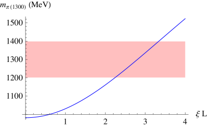
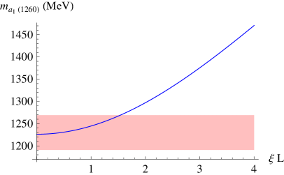
Figure 1: Mass of the $\pi(1300)$ meson (left) and $a_{1}(1260)$ meson (right) as a function of $\xi L$ for $L^{-1}=320\ {\rm MeV}$ and $L^{2}M_{Bulk}^{2}\simeq-3.8$. The shaded band shows the experimental values $m_{\pi(1300)}=(1300\pm 100)\ {\rm MeV}$ and $m_{a_{1}(1260)}=(1230\pm 40)\ {\rm MeV}$.

As can be seen from the plots in fig. 1, fitting the value of the $a_{1}(1260)$ mass points towards the region of small $\xi$, $\xi L\lesssim 2$, while reconstructing the $\pi(1300)$ mass favours larger value of the parameter $2\lesssim\xi L\lesssim 3$. Combining the two regions we get as a rough estimate $\xi L\simeq 2$. The values of $M_{5}$ and $M_{q}$ can be extracted respectively from the pion decay constant $f_{\pi}$ and the pion mass $m_{\pi}$. These two quantities can be determined by computing the holographic Lagrangian for the pion field as explained in appendix A. We find that the series expansion for small $\xi L$ is given by

$$f_{\pi}^{2}\simeq 4\frac{M_{5}}{L}\left(1+\frac{(\xi L)^{2}}{\Delta^{+}({\Delta^{+}}^{2}-1)}\right)\,,\qquad\quad m_{\pi}^{2}\simeq 2(\Delta^{+}-2)\xi M_{q}\,.$$ (36)

Using the experimental values $f_{\pi}^{2}=92\ {\rm MeV}$ and $m_{\pi}=135\ {\rm MeV}$, we get $M_{5}L\simeq 0.015$ and $M_{q}\simeq 35\ {\rm MeV}$.

A more precise determination of the microscopic parameters can be obtained by performing a fit on a larger set of well measured mesonic observables. This procedure provides also a way to estimate the level of agreement of the model with the experimental results. As a simple fitting procedure, we chose to minimize the root mean square error (RMSE) of our predictions with respect to the experimental data (see [10] for details on the fitting procedure). We remark that for our analysis we take into account only the deviation of the theoretical predictions of our model from the central value of the experimental results. A more refined procedure, which however would be beyond the scope of our work, should also take into account the experimental error with which the various observables have been measured.

	Experiment	AdS5	Deviat.
$m_{\pi}$	$135\ {\rm MeV}$	$134\ {\rm MeV}$	$0.6\%$
$m_{\pi(1300)}$	$1300\ {\rm MeV}$	$1230\ {\rm MeV}$	$5.6\%$
$m_{\rho}$	$775\ {\rm MeV}$	$783\ {\rm MeV}$	$1.0\%$
$m_{\omega}$	$782\ {\rm MeV}$	$783\ {\rm MeV}$	$0.1\%$
$m_{a_{1}(1260)}$	$1230\ {\rm MeV}$	$1320\ {\rm MeV}$	$7.6\%$
$m_{a_{0}(980)}$	$980\ {\rm MeV}$	$1040\ {\rm MeV}$	$6.5\%$
$m_{f_{0}(980)}$	$980\ {\rm MeV}$	$1040\ {\rm MeV}$	$6.5\%$
$f_{\pi}$	$92\ {\rm MeV}$	$89\ {\rm MeV}$	$3.6\%$
$f_{\rho}$	$153\ {\rm MeV}$	$149\ {\rm MeV}$	$2.7\%$
$f_{\omega}$	$140\ {\rm MeV}$	$149\ {\rm MeV}$	$6.4\%$
$g_{\rho\pi\pi}$	$6.0$	$4.89$	$22.7\%$
$g_{\omega\pi\gamma}$	$0.72$	$0.71$	$1.1\%$
$g_{\rho\pi\gamma}$	$0.22$	$0.24$	$7.9\%$
$g_{\omega\rho\pi}$	$15.0$	$15.6$	$3.7\%$
RMSE			$7.7\%$

	Experiment	AdS5	Deviat.
$m_{\pi}$	$135\ {\rm MeV}$	$133\ {\rm MeV}$	$1.2\%$
$m_{\pi(1300)}$	$1300\ {\rm MeV}$	$1207\ {\rm MeV}$	$7.7\%$
$m_{\rho}$	$775\ {\rm MeV}$	$842\ {\rm MeV}$	$8.6\%$
$m_{\omega}$	$782\ {\rm MeV}$	$842\ {\rm MeV}$	$7.7\%$
$m_{a_{1}(1260)}$	$1230\ {\rm MeV}$	$1387\ {\rm MeV}$	$12.7\%$
$m_{a_{0}(980)}$	$980\ {\rm MeV}$	$1099\ {\rm MeV}$	$12.1\%$
$m_{f_{0}(980)}$	$980\ {\rm MeV}$	$1099\ {\rm MeV}$	$12.1\%$
$f_{\pi}$	$92\ {\rm MeV}$	$89\ {\rm MeV}$	$3.1\%$
$f_{\rho}$	$153\ {\rm MeV}$	$158\ {\rm MeV}$	$3.1\%$
$f_{\omega}$	$140\ {\rm MeV}$	$158\ {\rm MeV}$	$12.7\%$
$g_{\rho\pi\pi}$	$6.0$	$5.33$	$12.5\%$
$g_{\omega\pi\gamma}$	$0.72$	$0.74$	$3.2\%$
$g_{\rho\pi\gamma}$	$0.22$	$0.25$	$12.6\%$
$g_{\omega\rho\pi}$	$15.0$	$16.8$	$11.8\%$
RMSE			$9.6\%$

Table 1: Meson observables used for the fit of the microscopic parameters. The table on the left shows the results of a fit which minimizes the overall root mean square error (shown in the last line). The values of the parameters obtained in this way are $L^{-1}=325\ {\rm MeV}$, $M_{5}L=0.014$, $L^{2}M^{2}_{Bulk}=-3.7$, $\xi L=2.1$ and $M_{q}=31\ {\rm MeV}$. The table on the right gives the list of results obtained by minimizing the largest deviation from the experiments. With this procedure we get $L^{-1}=350\ {\rm MeV}$, $M_{5}L=0.014$, $L^{2}M^{2}_{Bulk}=-3.8$, $\xi L=1.5$ and $M_{q}=40\ {\rm MeV}$.

The list of observables used in the fit includes the masses of the lightest mesonic resonances as well as some of their decay constants and couplings. The predictions of the model and the experimental values are shown in the list on the left of table 1. We found that the best agreement with the data is obtained for the following values of the parameters $L^{-1}=325\ {\rm MeV}$, $M_{5}L=0.014$, $L^{2}M^{2}_{Bulk}=-3.7$, $\xi L=2.1$ and $M_{q}=31\ {\rm MeV}$, which are close to the previously estimated ones. The overall agreement with the experimental data is quite good and almost all the observables show a deviation from the experimental values smaller than $8\%$, resulting in a RMSE of $7.7\%$. A somewhat surprising result of the fit is the fact that only one observable, namely the $g_{\rho\pi\pi}$ coupling seems to have a large deviation from the experiments. This deviation is however not completely unexpected. In the class of models we are considering one gets an approximate tree-level relation [3]

$$m_{\rho}^{2}\simeq 3f_{\pi}^{2}g_{\rho\pi\pi}^{2}\,,$$ (37)

which differ by a factor $2/3$ form the experimentally well satisfied KSRF relation $m_{\rho}^{2}\simeq 2f_{\pi}^{2}g_{\rho\pi\pi}^{2}$. In our fit the predictions for the pion decay constant and for the $\rho$ meson mass are in excellent agreement with the data, thus the $g_{\rho\pi\pi}$ coupling must necessarily deviate from the experiments in order for the relation (37) to be valid.

It is interesting to notice that the change in the IR boundary conditions for the gauge fields with respect to the original model of [4] has some relevant consequences on the predictions of the theory. In the original set-up the mass of the $\pi(1300)$ resonance could not be reproduced and the first resonance of the axial gauge field was identified with the $\pi(1800)$ state. In the present model, on the contrary, the $\pi(1300)$ meson can be naturally accomodated.

To check the stability of our predictions, we can compare the previous results with the ones obtained by using an alternative fitting procedure. For this purpose, we chose to minimize the largest deviation of our predictions from the experiments. In this way we obtained the list of result shown in the right panel of table 1. The deviations from the experiments are now more uniformly spread among the various observables, with a maximal deviation of $\sim 13\%$. The overall RMSE is $9.6\%$, which is still reasonable and only slightly higher than the one found in the previous fit. The corresponding values of the microscopic parameters are $L^{-1}=350\ {\rm MeV}$, $M_{5}L=0.014$, $L^{2}M^{2}_{Bulk}=-3.8$, $\xi L=1.5$ and $M_{q}=40\ {\rm MeV}$, which are in good agreement with the previous determination.

The heavier resonances, which have not been included in the fits, show larger deviations from the experimental values. For example the predicted mass for the $\pi(1800)$ is $2140\ {\rm MeV}$ with an $18\%$ deviation and for the $a_{0}(1450)$ it is $2070\ {\rm MeV}$ with a $40\%$ deviation. We remark, however, that the heavy resonances, being close to the cut-off of the theory, are expected to have larger theoretical uncertainties.

	Experiment	AdS5
$L_{1}$	$0.4\pm 0.3$	$0.47$
$L_{2}$	$1.4\pm 0.3$	$0.95$
$L_{3}$	$-3.5\pm 1.1$	$-2.8$
$L_{4}$	$-0.3\pm 0.5$	$0.0$
$L_{5}$	$1.4\pm 0.5$	$0.72$
$L_{6}$	$-0.2\pm 0.3$	$0.0$
$L_{8}$	$0.9\pm 0.3$	$0.45$
$L_{9}$	$6.9\pm 0.7$	$6.0$
$L_{10}$	$-5.5\pm 0.7$	$-6.0$

	Experiment	AdS5
$L_{1}$	$0.4\pm 0.3$	$0.43$
$L_{2}$	$1.4\pm 0.3$	$0.87$
$L_{3}$	$-3.5\pm 1.1$	$-2.4$
$L_{4}$	$-0.3\pm 0.5$	$0.0$
$L_{5}$	$1.4\pm 0.5$	$0.68$
$L_{6}$	$-0.2\pm 0.3$	$0.0$
$L_{8}$	$0.9\pm 0.3$	$0.39$
$L_{9}$	$6.9\pm 0.7$	$5.6$
$L_{10}$	$-5.5\pm 0.7$	$-5.6$

Table 2: Predictions for the coefficients of the ${\cal O}(p^{4})$ terms in the ${\bf\chi PT}$ Lagrangian compared with the experimental values [18]. The values are given in units of $10^{-3}$. The microscopic parameters are fixed by the fits on the observables in table 1 (RMSE fit for the left table and ‘maximal deviation’ fit for the right table).

Other quantities that we can extract from the model are the coefficients of the ${\cal O}(p^{4})$ terms in the ${\bf\chi PT}$ Lagrangian, which describe the interactions of the pions with the left and right sources and with the spurion field related to the quark masses. The computation can be performed by following the holographic procedure outlined in appendix A. Due to the non negligible experimental uncertainty, we decided not to include these observables in the fit for the microscopic parameters. We also excluded from the computation the $L_{7}$ coefficient which arises from integrating out the Goldstone boson singlet related to the $U(1)_{A}$ anomaly, whose complete treatment is not included in the present model (see footnote 3). In table 2 we listed the predictions of the model for two sets of microscopic parameters found with the RMSE and the ‘maximal deviation’ fit. The numerical results in the two cases are quite similar and show a good agreement with the experimental data. The reduced $\chi^{2}$ for the RMSE fit is $1.0$, while for the ‘maximal deviation’ fit it is $1.2$, and the deviations from the experimental data are always below $\sim 1.5\,\sigma$.

In the chiral-symmetric models without a bulk scalar field some phenomenologically successful relations were found among the coefficients of the ${\bf\chi PT}$ Lagrangian :

$$L_{2}=2L_{1}\,,\qquad L_{9}=-L_{10}\,,\qquad L_{4}=L_{6}=0\,,\qquad L_{3}=-6L_{1}\,.$$ (38)

In our set-up all these relations remain valid, except for the last one $L_{3}=-6L_{1}$, which receives some corrections but is still well satisfied (compare [3, 4]). Notice that the first and third relations in eq. (38), which are implied by the large $N_{c}$ limit of QCD [19], are not modified in our model.

3 Baryons From 5d Skyrmions

3.1 The Static Solution

In the present model, baryons arise as 5d Skyrmions and studying their properties requires a slight modification of the methods of [6, 7, 8], where the massless case has been considered. As a first step we will consider the static soliton configuration. A convenient and automatically consistent 2d ansatz is obtained, as in the massless case, by imposing the solution to be invariant under a certain set of symmetry transformations. These are cylindrical symmetry (i.e., the simultaneous action of $3$-space and $SU(2)_{V}$ rotations), 3d parity and time-inversion, defined as a change of sign of all the temporal components combined with ${\widehat{L}}\rightarrow-{\widehat{L}}$ and ${\widehat{R}}\rightarrow-{\widehat{R}}$. This leads to the following ansatz for the gauge fields

$$\left\{\begin{array}[]{l}\displaystyle{\overline{R}}^{a}_{j}({\bf x},z)=\displaystyle A_{1}(r,z){\widehat{x}}_{a}{\widehat{x}}_{j}+\frac{1}{r}\varepsilon_{ajk}{\widehat{x}}_{k}-\frac{\phi_{(x)}}{r}\varepsilon^{(x,y)}\Delta^{(y),aj}\,,\\ \displaystyle{\overline{R}}^{a}_{5}({\bf x},z)=\displaystyle A_{2}(r,z){\widehat{x}}^{a}\,,\\ \displaystyle\widehat{\overline{R}}_{0}({\bf x},z)=\displaystyle\frac{s(r,z)}{r}\,,\end{array}\right.$$ (39)

where $r^{2}=\sum_{i}x^{i}x^{i}$,   ${\widehat{x}}^{i}=x^{i}/r$, $\varepsilon^{(x,y)}$ is the antisymmetric tensor with $\varepsilon^{(1,2)}=1$ and the “doublet” tensors $\Delta^{(1,2)}$ are

$$\Delta^{(x),ab}\,=\,\left[\begin{array}[]{l}\epsilon^{abc}{\widehat{x}}^{c}\\ {\widehat{x}}^{a}{\widehat{x}}^{b}-\delta^{ab}\end{array}\right]\,.$$ (40)

Because of parity, eq. (39) also determines the ansatz for the ${\bf L}$ fields which are given by $L_{i}({\bf x},z)=-R_{i}(-{\bf x},z)$, $L_{5,0}({\bf x},z)=R_{5,0}(-{\bf x},z)$ and analogously for ${\widehat{L}}$, ${\widehat{R}}$.

The ansatz for $\Phi$ is obviously obtained by imposing the same symmetries: cylindrical symmetry implies

$$\overline{\Phi}({\bf x},z)=\omega_{0}(r,z)\frac{11}{2}+i\omega_{a}(r,z)\frac{\sigma^{a}}{2}\,,$$ (41)

where

$$\left\{\begin{array}[]{l}\omega_{0}(r,z)=\lambda_{2}(r,z)\,,\\ \rule{0.0pt}{15.00002pt}\omega_{a}(r,z)=\lambda_{1}(r,z)\,\widehat{x}_{a}\,.\end{array}\right.$$ (42)

It is easy to check that parity acts on $\Phi$ as $\Phi({\bf x},z,t)\rightarrow\Phi^{\dagger}(-{\bf x},z,t)$, while under time-inversion we have $\Phi({\bf x},z,t)\rightarrow\sigma_{2}\Phi^{*}({\bf x},z,-t)\sigma_{2}$. Imposing $\Phi$ to be invariant under these transformations simply implies that $\lambda_{1,2}$ are real. It is useful to note that our ansatz preserves, again as in the massless case, a local $U(1)$ subgroup of the original 5d chiral group corresponding to gauge transformations of the form $g_{R}=g$ and $g_{L}=g^{\dagger}$ with

$$g=\exp[i\alpha(r,z)x^{a}\sigma_{a}/(2r)]\,.$$ (43)

Under this residual $U(1)$ the fields $\phi=\phi_{1}+i\,\phi_{2}$, $s$ and $A_{\overline{\mu}}$ in eq. (39) are respectively one charged and one neutral scalar and a gauge field. It is easy to check that the field $\lambda=\lambda_{1}+i\,\lambda_{2}$ in eq. (41) also transforms as a charge-one scalar; it will be convenient to define its 2d covariant derivative as

$$D_{\bar{\mu}}\lambda\equiv\partial_{\bar{\mu}}\lambda-iA_{\bar{\mu}}\lambda\,.$$ (44)

It is straightforward to plug the ansatz in the 5d lagrangian and to obtain the energy of the Skyrmion. From the gauge part in eq. (8) and (9) we obtain, as in [7, 8],

$$\begin{array}[]{l}\displaystyle E_{G}=8\pi M_{5}\int_{0}^{\infty}dr\int^{z_{\rm\textsc{ir}}}_{z_{\rm\textsc{uv}}}dz\,\left\{a(z)\left[|D_{\bar{\mu}}\phi|^{2}+\frac{1}{4}r^{2}A^{2}_{\bar{\mu}\bar{\nu}}+\frac{1}{2r^{2}}\left(1-|\phi|^{2}\right)^{2}-\frac{1}{2}\left(\partial_{\bar{\mu}}s\right)^{2}\right]\right.\\ \displaystyle\left.-\frac{\gamma L}{2}\frac{s}{r}\epsilon^{\bar{\mu}\bar{\nu}}\bigg{[}\partial_{\bar{\mu}}(-i\phi^{*}D_{\bar{\nu}}\phi+h.c.)+A_{\bar{\mu}\bar{\nu}}\bigg{]}\right\}\,,\end{array}$$ (45)

where

$$\gamma\equiv\frac{N_{c}}{16\pi^{2}M_{5}L}\,,$$ (46)

while the new contribution coming from the scalar part in eq. (11) is

$$E_{\Phi}=8\pi M_{5}\int dr\int dz\left\{a^{3}(z)\left[\frac{r^{2}}{4}(D_{\bar{\mu}}\lambda)^{*}(D_{\bar{\mu}}\lambda)-\frac{1}{8}(\phi\lambda^{*}-\lambda\phi^{*})^{2}\right]+a^{5}(z)\frac{r^{2}}{4}M^{2}_{Bulk}\lambda^{*}\lambda\right\}\,.$$ (47)

Notice that the total energy $E=E_{G}+E_{\Phi}$ does not yet give the Skyrmion mass because the infinite energy of the vacuum needs to be subtracted in order to get an observable quantity. This zero-point energy is obtained from eq. (47) by plugging in the vacuum field configuration which is given by

$$\lambda\,=\,\lambda_{V}\,=\,2\,i\,v(z)\,,\quad\phi\,=\,\phi_{V}\,=-\,i\,,$$ (48)

all other fields vanishing.

The 2d EOM for the Skyrmion are easily derived, at this point, by varying the energy in eq. (45,47), but in order for them to be solved suitable boundary conditions need to be specified at the four boundaries ($z=z_{\rm\textsc{ir}}$, $z=z_{\rm\textsc{uv}}$, $r=0$ and $r\rightarrow\infty$) of our 2d space. At $z=z_{\rm\textsc{uv}}$ and $z=z_{\rm\textsc{ir}}$ the boundary conditions are given, up to the sign ambiguity in eq. (15) that we will now fix, by the ones discussed in the previous section. The presence of the $r=0$ boundary merely results from a choice of coordinates, the physical 5d space being completely regular at $r=0$. The boundary conditions will therefore result from just imposing regularity of the 5d fields, with no need for extra assumptions. At $r\rightarrow\infty$ we must require that the solution will have a finite mass, and this is ensured by imposing it to reduce, up to a symmetry transformation, to the vacuum configuration in eq. (48). We also want a $B=1$ solution, where the baryon charge $B$ is defined in eq. (1) and is given by

$$B=\frac{1}{2\pi}\int_{0}^{\infty}dr\int^{z_{\rm\textsc{ir}}}_{z_{\rm\textsc{uv}}}dz\,\epsilon^{\bar{\mu}\bar{\nu}}\bigg{[}\partial_{\bar{\mu}}(-i\phi^{*}D_{\bar{\nu}}\phi+h.c.)+F_{\bar{\mu}\bar{\nu}}\bigg{]}\,,$$ (49)

in terms of the 2d fields. The above equation can be easily rewritten (as it must, being the topological charge) as a 1d integral on the boundaries of the 2d space, and in order to get $B=1$ from the $r\rightarrow\infty$ boundary we must have, as in the massless case, the following boundary conditions

$${r\rightarrow\infty\ :\quad\left\{\displaystyle{\begin{array}[]{l}\displaystyle{\phi=-ie^{i\pi(z-z_{\rm\textsc{uv}})/(z_{\rm\textsc{ir}}-z_{\rm\textsc{uv}})}}\\ \displaystyle{A_{2}=\frac{\pi}{(z_{\rm\textsc{ir}}-z_{\rm\textsc{uv}})}}\\ \displaystyle{s=0}\end{array}}\right.\,,}$$ (50)

which are obtained from the vacuum (48) by means of a residual $U(1)$ transformation in the form of eq. (43), with $\alpha=\pi(z-z_{\rm\textsc{uv}})/(z_{\rm\textsc{ir}}-z_{\rm\textsc{uv}})$.

Consistently, the boundary conditions for $\lambda$ are obtained in the same way and read

$$r\rightarrow\infty\ :\quad\lambda\,=\,i\,e^{i\pi(z-z_{\rm\textsc{uv}})/(z_{\rm\textsc{ir}}-z_{\rm\textsc{uv}})}\,2\,v(z)\,.$$ (51)

At $z=z_{\rm\textsc{ir}}$, the above equation implies $\lambda(r=0,z=z_{\rm\textsc{ir}})=-2\,i\,\xi$, because the “twist” $e^{i\pi(z-z_{\rm\textsc{uv}})/(z_{\rm\textsc{ir}}-z_{\rm\textsc{uv}})}$ reduces to $-1$ at the IR while the vacuum respects the boundary condition (15) with the plus sign. This resolves the ambiguity and enforces the 5d Skyrmion to live in the minus-sign sector, with IR boundary conditions given by

$$z=z_{\rm\textsc{ir}}\ :\quad\lambda\,=\,-2\,i\,\xi\,.$$ (52)

We stress, as mentioned in the discussion below eq. (15), that the sign ambiguity in the IR boundary conditions results from our choice of giving generalized Dirichlet conditions on $\Phi$, instead of treating it as a Neumann field and making its boundary conditions originate from a localized potential that would cost us more new parameters. If we had made the other choice, we would have had no ambiguity, and consequently no separated sectors in the field space. If studying this different setup in the limit of infinite strength for the coupling in the localized potential we expect that, while the vacuum and the meson’s wave function will be found to fulfill eq. (15) with the plus sign, the other boundary condition will be enforced on the Skyrmion solution and the results of the present paper will be recovered. Coming back to the boundary conditions, we must still specify the ones at $r=0$ and at $z=z_{\rm\textsc{uv}}$. These are

$$r\rightarrow 0\ :\quad\left\{\begin{array}[]{l}\displaystyle{\lambda_{1}\,=\,0}\\ \displaystyle{\partial_{r}\lambda_{2}\,=\,0}\end{array}\right.\quad\qquad z=z_{\rm\textsc{uv}}\ :\quad\displaystyle{\lambda\,=\,2\,i\,\left(\frac{z_{\rm\textsc{uv}}}{z_{\rm\textsc{ir}}}\right)^{\Delta^{-}}\,M_{q}}$$ (53)

where the ones for $r=0$ arise, respectively, from asking the 5d field $\overline{\Phi}$ and its 3-space derivative to be regular and single-valued. For all the other fields the boundary conditions are the same of the massless case and are reported in appendix B.

3.2 Zero-Mode Fluctuations

In order to describe the baryons we need to consider the time-dependent deformations of the static soliton solution. The analysis proceeds exactly as in the massless case, we will therefore skip most of the details and refer the interested reader to ref. [8].

The single-baryon states can be identified with the zero-mode fluctuations, thus an analysis of the infinitesimal deformations will be sufficient for our purposes. The relevant configurations are the ones which describe a slowly-rotating solution, whose degrees of freedom can be parametrized by three collective coordinates encoded in an $SU(2)$ matrix $U(t)$.

To describe the solution we need to generalize the ansatze given in eqs. (39) and (41). The ansatz for the gauge fields is analogous to the one for the massless pion case:

$$R_{\hat{\mu}}({\bf x},z;U)\,=\,U\,{\overline{R}}_{\hat{\mu}}({\bf x},z)\,U^{\dagger}\,,\;\;\;\;\;\;\;\;\;{\widehat{R}_{0}}({\bf x},z;U)\,=\,{{{\widehat{\overline{R}}}}}_{0}({\bf x},z)\,,$$ (54)

and

$$R_{0}({\bf x},z;U)\,=\,U\,{\overline{R}}_{0}({\bf x},z;K)\,U^{\dagger}\,+\,i\,U\partial_{0}U^{\dagger}\,,\;\;\;\;\;\;\;\;\;{\widehat{R}_{\hat{\mu}}}({\bf x},z;U)\,=\,{{{\widehat{\overline{R}}}}}_{\hat{\mu}}({\bf x},z;K)\,,$$ (55)

where

$$\left\{\begin{array}[]{l}{\overline{R}}_{0}^{a}({\bf x},z;K)=\displaystyle\chi_{(x)}(r,z)k_{b}\Delta^{(x),ab}+w(r,z)(k\cdot{\widehat{x}}){\widehat{x}}^{a}\,,\\ \displaystyle{{{\widehat{\overline{R}}}}}_{i}({\bf x},z;K)=\displaystyle\frac{\rho(r,z)}{r}\left(k^{i}-(k\cdot{\widehat{x}}){\widehat{x}}^{i}\right)+B_{1}(r,z)(k\cdot{\widehat{x}}){\widehat{x}}^{i}+Q(r,z)\epsilon^{ibc}k_{b}{\widehat{x}}_{c}\,,\\ \displaystyle\rule{0.0pt}{15.00002pt}{{{\widehat{\overline{R}}}}}_{5}({\bf x},z;K)=\displaystyle B_{2}(r,z)(k\cdot{\widehat{x}})\,.\end{array}\right.$$ (56)

The ansatz for the scalar field $\Phi$ is given by

$$\Phi({\bf{x}},\,z;\,U)\,=\,U{\overline{\Phi}}({\bf{x}},\,z)\,U^{\dagger}\,,$$ (57)

where ${\overline{\Phi}}$ is as in eq. (41) with the new definitions

$$\left\{\begin{array}[]{l}\omega_{0}(r,z)=\exp\left[-i(k\cdot\widehat{x})\rho(r,z)\right]\left(\lambda_{2}(r,z)+i(k\cdot\widehat{x})\eta_{2}(r,z)\right)\,,\\ \rule{0.0pt}{15.00002pt}\omega_{a}(r,z)=\exp\left[-i(k\cdot\widehat{x})\rho(r,z)\right]\left[\left(\lambda_{1}(r,z)+i(k\cdot\widehat{x})\eta_{1}(r,z)\right)\widehat{x}^{a}-i\left((k\cdot\widehat{x})\widehat{x}^{a}-k^{a}\right)\zeta(r,z)\right]\,.\end{array}\right.$$ (58)

In the above equation, the 3-vector $k_{a}$ denotes the Skyrmion rotational velocity

$$K=k_{a}\sigma^{a}/2=-iU^{\dagger}dU/dt\,,$$

and the field $\rho$ is the same that appears in the ansatz for the gauge fields in eq. (56). The above ansatz can be obtained, similarly to the one for the static solution, by imposing time-inversion, parity, and cylindrical symmetry.

Plugging the ansatz in the 5d lagrangian one obtains the collective coordinates lagrangian

$$L=-M+\frac{\lambda}{2}\,k_{a}k^{a}\,,$$ (59)

where $M$ is the Skyrmion mass and $\lambda$ is its moment of inertia. The latter receives a contribution from the gauge Lagrangian

$$\displaystyle\lambda_{G} = 16\pi M_{5}\frac{1}{3}\int_{0}^{\infty}dr\int^{z_{\rm\textsc{ir}}}_{z_{\rm\textsc{uv}}}dz\,\left\{a(z)\left[-\left(D_{\bar{\mu}}\rho\right)^{2}-r^{2}\left(\partial_{\bar{\mu}}Q\right)^{2}-2Q^{2}-\frac{r^{2}}{4}B_{{\bar{\mu}}{\bar{\nu}}}B_{{\bar{\mu}}{\bar{\nu}}}\right.\right.$$ (60)

$$\displaystyle\left.\left.+r^{2}\left(D_{\bar{\mu}}\chi\right)^{2}+\frac{r^{2}}{2}\left(\partial_{\bar{\mu}}w\right)^{2}+\left(\chi_{(x)}\chi_{(x)}+w^{2}\right)\left(1+\phi_{(x)}\phi_{(x)}\right)-4w\phi_{(x)}\chi_{(x)}\right]\right.$$

$$\displaystyle\left.+\gamma L\bigg{[}-2\epsilon^{\bar{\mu}\bar{\nu}}D_{\bar{\mu}}\rho\,\chi_{(x)}\left(D_{\bar{\nu}}\phi\right)_{(x)}+2\epsilon^{\bar{\mu}\bar{\nu}}\partial_{\bar{\mu}}\left(r\,Q\right)\,\chi_{(x)}\epsilon^{(xy)}\left(D_{\bar{\nu}}\phi\right)_{(y)}\right.$$

$$\displaystyle\left.-w\left(\frac{1}{2}\epsilon^{\bar{\mu}\bar{\nu}}B_{\bar{\mu}\bar{\nu}}\left(\phi_{(x)}\phi_{(x)}-1\right)+r\,Q\epsilon^{\bar{\mu}\bar{\nu}}A_{\bar{\mu}\bar{\nu}}\right)+2r\,Q\epsilon^{\bar{\mu}\bar{\nu}}D_{\bar{\mu}}\rho\partial_{\bar{\nu}}\left(\frac{s}{r}\right)\bigg{]}\right\}\,,$$

and a contribution from the scalar, which is given by

$$\lambda_{\Phi} = \frac{16}{3}\pi M_{5}\int_{0}^{\infty}dr\int_{z_{\rm\textsc{uv}}}^{z_{\rm\textsc{ir}}}dz\left\{a^{3}(z)\left[-\frac{r^{2}}{4}\lambda^{*}\lambda(D_{\bar{\mu}}\rho)(D_{\bar{\mu}}\rho)-\frac{r^{2}}{4}(D_{\bar{\mu}}\eta)^{*}(D_{\bar{\mu}}\eta)-\frac{r^{2}}{2}(\partial_{\bar{\mu}}\zeta)(\partial_{\bar{\mu}}\zeta)\right.\right.$$ (61)

$$+\frac{r^{2}}{4}D_{\bar{\mu}}\rho\left[\lambda(D_{\bar{\mu}}\eta)^{*}-\eta(D_{\bar{\mu}}\lambda)^{*}+{\rm h.c.}\right]-\frac{1}{2}\eta^{*}\eta+\frac{1}{8}(\eta\phi^{*}-\phi\eta^{*})^{2}-\frac{r^{2}}{8}(\chi\lambda^{*}-\lambda\chi^{*})^{2}$$

$$\left.\left.-i\zeta(\eta\phi^{*}-\phi\eta^{*})-\frac{1}{2}\zeta^{2}(1+\phi^{*}\phi)\right]-r^{2}a^{5}(z)M^{2}_{Bulk}\left[\frac{1}{4}\eta^{*}\eta+\frac{1}{2}\zeta^{2}\right]\right\}\,,$$

where we defined

$$\eta=\eta_{1}+i\eta_{2}\,,\qquad\qquad D_{\bar{\mu}}\eta\equiv\partial_{\bar{\mu}}\eta-iA_{\bar{\mu}}\eta\,.$$ (62)

while the other notations are defined in appendix B.

3.3 Numerical Results

The soliton solution can not be determined analytically, however, it can be studied numerically by using the techniques described in [8]. In the massless case it was found that, due to the peculiarity of the $5$d gauge action, the soliton solution is stabilized thanks to the presence of the CS term [7]. This peculiar feature disappears once we modify the action by the introduction of the bulk scalar field and, in the present model, we checked in our numerical analysis that the Skyrmion size is stable even if the CS term is not present.

From the soliton solution we can extract the electromagnetic and axial properties of the nucleons, which are encoded in a set of form factors which parametrize the matrix element of the currents on two nucleon states.

The chiral currents can be determined by computing the variation of the action with respect to the sources ${\bf l}_{\mu}$ and ${\bf r}_{\mu}$. It is simple to show that the action describing the scalar field $\Phi$ does not contribute to the currents, which are exactly the same as in the massless pion case:

$$J_{L\,\mu}^{a}\,=\,M_{5}\big{(}a(z)L_{\mu\,5}^{a}\big{)}\left|{}_{z=z_{\rm\textsc{uv}}}\right.\ ,\;\;\;\;\;{\widehat{J}}_{L\,\mu}\,=\,M_{5}\big{(}a(z){\widehat{L}}_{\mu\,5}\big{)}\left|{}_{z=z_{\rm\textsc{uv}}}\right.\,,$$ (63)

and analogously for $R$.

The isoscalar and isovector form factors are defined through the relations

$$\displaystyle\langle N_{f}({\vec{q}}/2)|J^{0}_{S}(0)|N_{i}(-{\vec{q}}/2)\rangle = G_{E}^{S}({\vec{q}\,}^{2})\chi_{f}^{\dagger}\chi_{i}\,,$$

$$\displaystyle\langle N_{f}({\vec{q}}/2)|J^{i}_{S}(0)|N_{i}(-{\vec{q}}/2)\rangle = i\,\frac{G_{M}^{S}({\vec{q}\,}^{2})}{2M_{N}}\chi_{f}^{\dagger}2({\vec{S}}\times{\vec{q}})^{i}\chi_{i}\,,$$

$$\displaystyle\langle N_{f}({\vec{q}}/2)|J^{0a}_{V}(0)|N_{i}(-{\vec{q}}/2)\rangle = G_{E}^{V}({\vec{q}\,}^{2})\chi_{f}^{\dagger}\left(2I^{a}\right)\chi_{i}\,,$$

$$\displaystyle\langle N_{f}({\vec{q}}/2)|J^{ia}_{V}(0)|N_{i}(-{\vec{q}}/2)\rangle = i\,\frac{G_{M}^{V}({\vec{q}\,}^{2})}{2M_{N}}\chi_{f}^{\dagger}2({\vec{S}}\times{\vec{q}})^{i}\left(2I^{a}\right)\chi_{i}\,,$$ (64)

where the currents are given by $J_{V}^{a}=J_{R}^{a}+J_{L}^{a}$ and $J_{S}=1/3({\widehat{J}}_{R}+{\widehat{J}}_{L})$, and we used the notation $\chi_{i,f}$ for the nucleon spin/isospin vectors of state (normalized to $\chi^{\dagger}\chi=1$) and the definition $({\vec{S}}\times{\vec{q}})^{i}\equiv\varepsilon^{ijk}S^{j}q^{k}$. From the axial current $J_{A}^{a}=J_{R}^{a}-J_{L}^{a}$, we define the axial form factors

$$\langle N_{f}({\vec{q}}/2)|J_{A}^{i,a}(0)|N_{i}(-{\vec{q}}/2)\rangle = \chi_{f}^{\dagger}\!\left[\frac{E}{M_{N}}G_{A}({\vec{q}\,}^{2})S^{i}_{T}+\!\left(\!G_{A}({\vec{q}\,}^{2})-\frac{{\vec{q}\,}^{2}}{4M_{N}^{2}}G_{p}({\vec{q}\,}^{2})\right)\!\!S^{i}_{L}\right]\!\!I^{a}\chi_{i}\,,\hskip 15.00002pt$$ (65)

$$\langle N_{f}({\vec{q}}/2)|J_{A}^{0,a}(0)|N_{i}(-{\vec{q}}/2)\rangle = 0$$ (66)

where ${\vec{S}}_{T}\equiv{\vec{S}}-\hat{{\vec{q}}}\ {\vec{S}}\cdot{\hat{\vec{q}}}$ and ${\vec{S}}_{L}\equiv\hat{{\vec{q}}}\ {\vec{S}}\cdot{\hat{\vec{q}}}$ are the transverse and the longitudinal components of the spin operator.

To find the explicit expressions for the form factors we need to plug the ansatze for the soliton solution into the definitions of the currents (63) and then perform the quantization of the soliton solution as explained in [8]. The result is the same as in the massless pion case:

$$G_{E}^{S}\,=\,-\frac{N_{c}}{6\pi\gamma L}\int dr\,r\,j_{0}(qr)\left(a(z)\partial_{z}s\right)_{UV}$$

$$G_{E}^{V}\,=\,\frac{4\pi M_{5}}{3\lambda}\int dr\,r^{2}\,j_{0}(qr)\left[a(z)\left(\partial_{z}w-2\left(D_{z}\chi\right)_{(2)}\right)\right]_{UV}$$

$$G_{M}^{S}\,=\,\frac{8\pi M_{N}M_{5}}{3\lambda}\int dr\,r^{3}\,\frac{j_{1}(qr)}{qr}\left(a(z)\partial_{z}Q\right)_{UV}$$

$$G_{M}^{V}\,=\,\frac{M_{N}\,N_{c}}{3\pi L\gamma}\int dr\,r^{2}\,\frac{j_{1}(qr)}{qr}\left(a(z)\left(D_{z}\phi\right)_{(2)}\right)_{UV}$$

$$G_{A}\,=\,\frac{M_{N}}{E}\frac{N_{c}}{3\pi\gamma L}\int dr\,r\left[a(z)\frac{j_{1}(qr)}{qr}\left(\left(D_{z}\phi\right)_{(1)}-r\,A_{zr}\right)-a(z)\left(D_{z}\phi\right)_{(1)}j_{0}(qr)\right]_{UV}$$ (67)

where $j_{n}$ are spherical Bessel functions.

	Experiment	AdS5	Deviat.
$M_{N}$	$940\ {\rm MeV}$	$1090\ {\rm MeV}$	$16\%$
$\mu_{S}$	$0.44$	$0.43$	$2\%$
$\mu_{V}$	$2.35$	$1.18$	$100\%$
$g_{A}$	$1.25$	$0.58$	$100\%$
$\sqrt{\langle r^{2}_{E,S}\rangle}$	$0.79\ {\rm fm}$	$0.82\ {\rm fm}$	$4\%$
$\sqrt{\langle r^{2}_{E,V}\rangle}$	$0.93\ {\rm fm}$	$0.97\ {\rm fm}$	$4\%$
$\sqrt{\langle r^{2}_{M,S}\rangle}$	$0.82\ {\rm fm}$	$0.84\ {\rm fm}$	$2\%$
$\sqrt{\langle r^{2}_{M,V}\rangle}$	$0.87\ {\rm fm}$	$0.87\ {\rm fm}$	$0.5\%$
$\sqrt{\langle r^{2}_{A}\rangle}$	$0.68\ {\rm fm}$	$0.65\ {\rm fm}$	$5\%$

	Experiment	AdS5	Deviat.
$M_{N}$	$940\ {\rm MeV}$	$1104\ {\rm MeV}$	$17\%$
$\mu_{S}$	$0.44$	$0.43$	$3\%$
$\mu_{V}$	$2.35$	$1.15$	$100\%$
$g_{A}$	$1.25$	$0.59$	$100\%$
$\sqrt{\langle r^{2}_{E,S}\rangle}$	$0.79\ {\rm fm}$	$0.84\ {\rm fm}$	$6\%$
$\sqrt{\langle r^{2}_{E,V}\rangle}$	$0.93\ {\rm fm}$	$1.02\ {\rm fm}$	$9\%$
$\sqrt{\langle r^{2}_{M,S}\rangle}$	$0.82\ {\rm fm}$	$0.86\ {\rm fm}$	$5\%$
$\sqrt{\langle r^{2}_{M,V}\rangle}$	$0.87\ {\rm fm}$	$0.86\ {\rm fm}$	$1\%$
$\sqrt{\langle r^{2}_{A}\rangle}$	$0.68\ {\rm fm}$	$0.68\ {\rm fm}$	$0.2\%$

Table 3: Prediction for the static nucleon observables with the parameter values fixed by the fit on the mesonic observables (RMSE fit for the left table and ‘maximal deviation’ fit for the right table).

By employing suitable numerical techniques, the 2d EOM obtained by varying the soliton mass $M$ and its moment of inertia $\lambda$ can be solved, and both the static and slowly-rotating Skyrmion solution computed. The numerical predictions for the static nucleon observables are listed in table 3. In the analysis we used the values of the microscopic parameters obtained from the fits on the mesonic observables presented in section 2.2.

The numerical results for the two sets of microscopic parameters considered show very similar deviation patterns from the data. Many of the numerical predictions are very close to the experimental results, although the magnetic vector moment $\mu_{V}$ and the axial coupling $g_{A}$ present a deviation of order $100\%$. We notice, however, that the overall agreement with the data (root mean square error $~{}45\%$) is still compatible with the possibility of having sizable $1/N_{c}$ corrections, which can not be excluded given that $N_{c}=3$. By comparing the present results with the ones found in the simplified model without a pion mass [8], we see that all the observables show an improved agreement with the data except for the $\mu_{V}$ and $g_{A}$, whose deviations become significantly larger.

Form the qualitative point of view, we remark that an important check of the validity of the description of baryons as solitons is the behavior of the electric and magnetic vector radii, namely $r_{E,V}$ and $r_{M,V}$. These two quantities are expected to be divergent in the chiral limit, as explicitly verified in [8], while they should become finite once a pion mass is introduced, as we find in the present model.

4 Conclusions

We have shown that it is rather easy to construct a model of holographic QCD which describes at the same time the pion mass, the QCD anomalies and the baryons as topological solitons. After introducing an explicit minimal model we have studied its phenomenology in both the mesonic and baryonic sector and found a significant level of agreement. In extreme synthesis, our result is that the general picture on the holographic QCD models outlined in the Introduction survives unchanged to the inclusion of the pion mass.

Few unexpected results have been found, however, that is worth discussing. In Sect. 2 we saw that our model easily reproduces the mass of the $\pi(1300)$ meson, a task that was impossible to achieve in the original scenario [4]. This came because of the change in the IR boundary conditions and gives a phenomenological support to this modification, that we had instead motivated on purely theoretical grounds. It is also remarkable that the other predictions are almost unaffected so that all the valid phenomenology of the original construction is retained. The “new” observables that were absent in the original model, i.e. the anomalous parity couplings originating from the CS term, also show a good agreement with the observations. Our results in the baryonic sector, shown in table 3, are also surprising, especially if compared with the ones obtained in the chiral-symmetric case [6, 7, 8]. For all the observables except $\mu_{V}$ and $g_{A}$, a significant improvement is found in the agreement with observations. The isovector radii, that have became finite due to the presence of the pion mass, are also extremely well predicted. The situation has got significantly worst, on the contrary, for $\mu_{V}$ and $g_{A}$ that have became a factor of $2$ smaller than the observations. This failure persists in both the best fit points that we have used as input parameters in table 3, so that it is probably a robust feature. It might signal that the model is incomplete, but it might also be attributed to anomalously large $1/N_{c}$ corrections.

Some final comments on the theoretical implications of our results. The microscopic origin of holographic QCD models is basically unknown, even though the holographic implementation of the chiral symmetry provides a robust (but purely technical) connection with AdS/CFT. The success of the Regge phenomenology suggests, independently of AdS/CFT, the dual of large-$N_{c}$ QCD being a string model and the validity of the holographic QCD approach suggests that this string model should contain a sector that is well described by a 5d field theory similar to the one we have considered. In the case of exact chiral symmetry, the Sakai–Sugimoto model [21, 22] provides a partial realization of this idea because it is equivalent to holographic QCD for what the physics of the light meson is concerned. It is on the contrary different, and problematic, in the baryonic sector [6, 7, 8, 12] and its phenomenology in the sector of higher spin states (where it genuinely differs from holographic QCD and shows its stringy nature) seems not very promising [22]. The inclusion of the explicit chiral breaking considered in the present paper provides an additional piece of information. The chiral symmetry is not explicitly broken in Sakai–Sugimoto, and even though it was possible to include the explicit breaking by some deformation, the resulting model could not reduce to a field-theoretical model such as the one we have considered. The reason for this is that the Left and Right global groups are localized, in Sakai–Sugimoto, at two different boundaries of the 5d space and the quark mass spurion $M$ is unavoidably a non local object which is impossible to describe in a field theoretical language. Therefore, any string model that incorporated ours, inheriting its phenomenology, would be deeply different from Sakai–Sugimoto; it might be worth trying to construct one following a bottom–up approach.

Appendix A The Effective Action for the Pion

In this appendix we will compute the effective action for the pion at ${\cal O}(p^{4})$. Given that a complete treatment of the $U(1)_{A}$ anomaly is not included in the model, in the following we will neglect the Goldstone boson related to this symmetry, namely the $\eta^{\prime}$ field, and we will only consider a model with a chiral symmetry $SU(2)_{L}\times SU(2)_{R}$.

An efficient way to perform the computation is to use the holographic approach presented in [14]. At tree-level, the holographic action for the pion is given by the 5d action for the gauge and the scalar fields (eqs. (8) and (11)), where the 5d fields satisfy the bulk EOM’s with the usual IR boundary conditions given in eqs. (14) and (15). The UV conditions are modified as

$$\left\{\begin{array}[]{l}\left.L_{\mu}\right|_{z_{\rm\textsc{uv}}}=U(x)(l_{\mu}+i\partial_{\mu})U(x)^{\dagger}\\ \left.R_{\mu}\right|_{z_{\rm\textsc{uv}}}=r_{\mu}\\ \left.\Phi\right|_{z_{\rm\textsc{uv}}}=U(x)\left(\frac{z_{\rm\textsc{uv}}}{z_{\rm\textsc{ir}}}\right)^{\Delta_{-}}M_{q}11\end{array}\right.\,,$$ (68)

where $U(x)$ represents the 4d Goldstone matrix, which transforms as

$$U(x)\rightarrow g_{R}U(x)g_{L}^{\dagger}$$ (69)

under a chiral $SU(2)_{L}\times SU(2)_{R}$ 4d transformation. Notice that we are not interested in possible terms involving the scalar and pseudoscalar sources, so we did not include any source term in the UV condition for the scalar field in eq. (68).

To derive the complete effective action for the pion one would need to solve the full bulk EOM for the 5d fields. However, due to the presence of interaction terms, this can be done only perturbatively. As usually done in ${\bf\chi PT}$, we use an expansion in powers of the momentum $p$ and we treat the external sources $l_{\mu}$ and $r_{\mu}$ as ${\cal O}(p)$ terms, while $M_{q}$ will be treated as an ${\cal O}(p^{2})$ term.

We expand the solutions of the EOM using a mixed momentum–space representation

$$\left\{\begin{array}[]{l}V_{\mu}=f_{V}^{0}(z)\widehat{V}_{\mu}(p)+V^{(3)}_{\mu}(p,z,\widehat{V},\widehat{A},U,M_{q})\,,\\ \rule{0.0pt}{12.50002pt}A_{\mu}=f_{A}^{0}(z)\widehat{A}_{\mu}(p)+A^{(3)}_{\mu}(p,z,\widehat{V},\widehat{A},U,M_{q})\,,\\ \rule{0.0pt}{12.50002pt}\Phi=\Phi^{(0)}(z)+\Phi^{(2)}(p,z,\widehat{V},\widehat{A},U,M_{q})+\Phi^{(4)}(p,z,\widehat{V},\widehat{A},U,M_{q})\,,\end{array}\right.$$ (70)

where we denoted by $\widehat{V}$ and $\widehat{A}$ the values of the vector and axial gauge fields at the UV boundary. Notice that, due to the tensorial structure, the gauge field solutions start at ${\cal O}(p)$ and their next to leading terms are of ${\cal O}(p^{3})$, while the scalar field can be expanded in terms of ${\cal O}(p^{2n})$. All the terms in the expansion of the gauge fields satisfy the same IR boundary conditions as the original fields:

$$\left\{\begin{array}[]{l}\partial_{z}V_{\mu}(x,z_{\rm\textsc{ir}})=0\,,\\ \rule{0.0pt}{12.50002pt}A_{\mu}(x,z_{\rm\textsc{ir}})=0\,.\end{array}\right.$$ (71)

Instead, for the scalar field we have

$$\left\{\begin{array}[]{l}\Phi^{(0)}(x,z_{\rm\textsc{ir}})=\xi 11\,,\\ \rule{0.0pt}{12.50002pt}\Phi^{(i)}(x,z_{\rm\textsc{ir}})=0\qquad{\rm for\ }i\geq 2\,.\end{array}\right.$$ (72)

The UV boundary conditions for the gauge fields are chosen so that the higher terms in the expansion vanish, while for the leading terms we have

$$f_{V,A}^{0}(z_{\rm\textsc{uv}})=1\,.$$ (73)

For the scalar field we impose

$$\left\{\begin{array}[]{l}\Phi^{(0)}(z_{\rm\textsc{uv}})=0\,,\\ \rule{0.0pt}{12.50002pt}\Phi^{(2)}(z_{\rm\textsc{uv}})=\displaystyle U\left(\frac{z_{\rm\textsc{uv}}}{z_{\rm\textsc{ir}}}\right)^{\Delta_{-}}M_{q}11\,,\\ \rule{0.0pt}{12.50002pt}\Phi^{(4)}(z_{\rm\textsc{uv}})=0\qquad{\rm for\ }i\geq 4\,.\end{array}\right.$$ (74)

By using the bulk EOM’s and the boundary conditions for the fields, one can verify that the terms of ${\cal O}(p^{3})$ in the expansion for the gauge fields and the ones of order ${\cal O}(p^{4})$ in the expansion for the scalar field do not contribute to the effective action for the pion at ${\cal O}(p^{4})$ (see the discussion in [14]).

As a first step of the derivation of the effective action, we will consider the contributions coming from the 5d gauge action in eq. (8). It is convenient to rewrite eq. (8) in the form

$$S_{g} = -2M_{5}\int_{UV}d^{4}x\ a(z_{\rm\textsc{uv}})\,{\rm Tr}\left[V_{\mu}\partial_{z}V^{\mu}+A_{\mu}\partial_{z}A^{\mu}\right]$$ (75)

$$-M_{5}\int d^{4}x\ \int dza(z)\,{\rm Tr}\left[L_{\mu\nu}L^{\mu\nu}+R_{\mu\nu}R^{\mu\nu}\right]\,.$$

The leading terms in the expansion of the 5d fields satisfy the equations

$$\left\{\begin{array}[]{l}\partial_{z}\left(a(z)\partial_{z}f^{0}_{V}(z)\right)=0\,,\\ \rule{0.0pt}{12.50002pt}\partial_{z}\left(a(z)\partial_{z}f^{0}_{A}(z)\right)-2a^{3}(z)(\Phi^{(0)})^{2}f^{0}_{A}(z)=0\,,\\ \rule{0.0pt}{12.50002pt}\partial_{z}\left(a^{3}(z)\partial_{z}\Phi^{(0)}(z)\right)-a^{5}(z)M_{\phi}^{2}\Phi^{(0)}(z)=0\,.\end{array}\right.$$ (76)

The solution for the $\Phi^{(0)}$ field can be obtained from eqs. (17) and (18) by setting $M_{q}=0$. The equation for the vector gauge field admits the simple solution $f_{V}^{0}(z)=1$, while the equation for $f_{A}^{0}$ in general can not be solved analytically.

By substituting the above expressions in the gauge action and using the relation

$$\widehat{A}_{\mu}=\frac{i}{2}U\left(D_{\mu}U\right)^{\dagger}=-\frac{i}{2}\left(D_{\mu}U\right)U^{\dagger}\equiv u_{\mu}\,,$$ (77)

we find that the first line in eq. (75) gives the kinetic term for the pion, from which we can extract the pion decay constant

$$f_{\pi}^{2}=\left.-2M_{5}a(z)\partial_{z}f_{A}^{0}(z)\right|_{z=z_{\rm\textsc{uv}}}\,.$$ (78)

From the second line in eq. (75) we get contributions to the ${\cal O}(p^{4})$ terms in the pion effective Lagrangian. In the standard form of ${\bf\chi PT}$ [19] we get the following contributions

$$\left\{\begin{array}[]{l}L_{1}^{(g)}=\displaystyle\frac{M_{5}}{16}\int dz\,a(z)\left(1-(f_{A}^{0})^{2}\right)^{2}\\ \rule{0.0pt}{15.00002pt}L_{10}^{(g)}=\displaystyle-\frac{M_{5}}{2}\int dz\,a(z)\left(1-(f_{A}^{0})^{2}\right)\end{array}\right.\,,\qquad\left\{\begin{array}[]{l}L_{2}^{(g)}=2L_{1}^{(g)}\\ L_{3}^{(g)}=-6L_{1}^{(g)}\\ L_{9}^{(g)}=-L_{10}^{(g)}\end{array}\right.\,.$$ (79)

Now we consider the contributions to the effective action coming from the scalar action in eq. (11). To derive the action we need to compute the $\Phi^{(2)}$ term in the expansion of the 5d scalar field. This term satisfies the bulk EOM

$$-\frac{1}{a^{3}(z)}\partial_{z}\left(a^{3}(z)\partial_{z}\Phi^{(2)}\right)+a^{2}(z)M_{\phi}^{2}\Phi^{(2)}=-2\Phi^{(0)}\left[-2(f_{A}^{0})^{2}u_{\mu}u^{\mu}-if_{A}^{0}D_{\mu}u^{\mu}\right]\,,$$ (80)

where we defined $D_{\mu}u^{\mu}\equiv\partial_{\mu}u^{\mu}-i[\widehat{V}_{\mu},u^{\mu}]$. The solution can be split into two parts:

$$\Phi^{(2)}=\Phi^{(2)}_{M}+\Phi^{(2)}_{0}\,,$$ (81)

where $\Phi^{(2)}_{M}$ is a solution of the homogeneous part of eq. (80) with boundary conditions

$$\Phi^{(2)}_{M}(z_{\rm\textsc{uv}})=\displaystyle U\left(\frac{z_{\rm\textsc{uv}}}{z_{\rm\textsc{ir}}}\right)^{\Delta_{-}}M_{q}11\,,\qquad\Phi^{(2)}_{M}(z_{\rm\textsc{ir}})=0\,,$$ (82)

while $\Phi^{(2)}_{0}$ satisfies eq. (80) with boundary conditions

$$\Phi^{(2)}_{0}(z_{\rm\textsc{uv}})=\Phi^{(2)}_{0}(z_{\rm\textsc{ir}})=0\,.$$ (83)

The solution for $\Phi^{(0)}_{M}$ is simply given by eqs. (17) and (18) with the choice $\xi=0$. The solution for $\Phi^{(0)}_{0}$ can not be found analytically, and we will parametrize it as

$$\Phi^{(0)}_{0}=f_{R}^{(2)}(z)u_{\mu}u^{\mu}+f_{I}^{(2)}(z)D_{\mu}u^{\mu}\,.$$ (84)

From the action for the scalar field we get an ${\cal O}(p^{2})$ contribution to the pion effective action, which can be written as

$$S_{\phi}^{(2)}=M_{5}\int_{UV}d^{4}x\,a^{3}(z){\rm Tr}\left[{\Phi^{(2)}_{M}}^{\dagger}\partial_{z}\Phi^{(0)}+{\rm h.c.}\right]\,.$$ (85)

To obtain this expression we integrated by parts the terms containing derivatives with respect to $z$ and we used the bulk EOM and the boundary conditions for the terms in the scalar field expansion. Eq. (85) corresponds to a mass term for the pion, which in the limit $z_{\rm\textsc{uv}}\rightarrow 0$ becomes

$$S_{\phi}^{(2)}=2\frac{M_{5}}{L}\,\alpha\,\xi\int d^{4}x\,{\rm Tr}\left[UM_{q}^{\dagger}+M_{q}U^{\dagger}\right]\,.$$ (86)

The expression for the pion mass and for the pion decay constant can be easily computed as an expansion in the parameter $\xi$. Some approximate expressions are reported in eq. (36).

Computing the ${\cal O}(p^{4})$ terms in the action we get

$$S_{\phi}^{(4)} = M_{5}\int d^{4}x\int dz\,a^{3}(z)\Big{\{}2{\rm Tr}\left[\Phi^{(0)}f_{I}^{(2)}(z)f_{A}^{0}(z)D_{\mu}u^{\mu}D_{\nu}u^{\nu}\right]$$ (87)

$$\hskip 95.00014pt+4{\rm Tr}\left[\Phi^{(0)}f_{R}^{(2)}(z)(f_{A}^{0}(z))^{2}u_{\mu}u^{\mu}u_{\nu}u^{\nu}\right]$$

$$\hskip 95.00014pt+i{\rm Tr}\left[\Phi^{(0)}\left({\Phi^{(2)}_{M}}^{\dagger}-{\Phi^{(2)}_{M}}\right)f_{A}^{0}(z)D_{\mu}u^{\mu}\right]$$

$$\hskip 95.00014pt+2{\rm Tr}\left[\Phi^{(0)}\left({\Phi^{(2)}_{M}}^{\dagger}+{\Phi^{(2)}_{M}}\right)(f_{A}^{0}(z))^{2}u_{\mu}u^{\mu}\right]\Big{\}}$$

$$+\frac{M_{5}}{2}\int_{UV}d^{4}x\,a^{3}(z){\rm Tr}\left[\partial_{z}(f_{R}^{(2)}(z)u_{\mu}u^{\mu}-if_{I}^{(2)}(z)D_{\mu}u^{\mu})\Phi^{(2)}_{M}+{\rm h.c.}\right]\,.$$

The ${\cal O}(p^{4})$ action for the pion can be simplified by using the EOM for the pion field coming from the ${\cal O}(p^{2})$ effective action. Using the standard notation of ${\bf\chi PT}$ [19], the kinetic and mass terms for the pion are written as

$${\cal L}=\frac{f_{\pi}^{2}}{4}\left\{{\rm Tr}\left[(D_{\mu}U)^{\dagger}D^{\mu}U\right]+{\rm Tr}\left(\chi^{\dagger}U+\chi U^{\dagger}\right)\right\}\,.$$ (88)

From this Lagrangian we get the EOM for $U$:

$$(D_{\mu}D^{\mu}U)U^{\dagger}-U(D_{\mu}D^{\mu}U)^{\dagger}+U\chi^{\dagger}-\chi U^{\dagger}=0\,,$$ (89)

which can be rewritten as

$$4iD_{\mu}u^{\mu}=\chi U^{\dagger}-U\chi^{\dagger}\,.$$ (90)

Moreover, by comparing eq. (88) and eq. (86), we can extract the relation between $M_{q}$ and $\chi$, which, in the $z_{\rm\textsc{uv}}\rightarrow 0$, limit reads

$$M_{q}=\frac{L}{M_{5}\alpha\xi}\frac{f_{\pi}^{2}}{8}\chi\,.$$ (91)

By using these relations we get the scalar contributions to the coefficients of the ${\cal O}(p^{4})$ effective pion action

$$\left\{\begin{array}[]{l}L_{3}^{(\phi)}=\displaystyle\frac{M_{5}}{8}\int dz\ a^{3}(z){\rm Tr}\left(\Phi^{(0)}\right)f_{R}^{(2)}(z)(f_{a}^{0}(z))^{2}\,,\\ L_{5}^{(\phi)}=\displaystyle\frac{\kappa M_{5}}{8}\left\{\left.a^{3}(z)f_{M}^{(2)}(z)\partial_{z}f_{R}^{(2)}(z)\right|_{z_{\rm\textsc{uv}}}\!\!+2\!\!\int dz\ a^{3}(z)f_{M}^{(2)}(z)(f_{a}^{0}(z))^{2}{\rm Tr}\left(\Phi^{(0)}\right)\right\}\,,\\ L_{8}^{(\phi)}=\displaystyle\frac{M_{5}}{16}\left\{\!\left.2\kappa a^{3}(z)f_{M}^{(2)}(z)\partial_{z}f_{I}^{(2)}(z)\right|_{z_{\rm\textsc{uv}}}\!\!-\!\!\int dz\ a^{3}(z)f_{a}^{0}(z)(f_{I}^{(2)}(z)-2\kappa f_{M}^{(2)}(z)){\rm Tr}\left(\Phi^{(0)}\right)\right\}\,,\end{array}\right.$$ (92)

where $\kappa$ is defined by the relation $M_{q}=\kappa\chi$.

Appendix B The Equations of Motion

In this appendix we report the EOM for the 2d fields which appear in the ansatz for the zero-mode soliton fluctuations in eqs. (39), (56) and (58), and we summarize the notation used in the paper.

B.1 The Equations of Motion

Before writing the EOM’s for the 2d fields, it is useful to recall the residual symmetries which survive after we choose the ansatze for the Skyrmion solution. As already discussed in sec. 3.1, the ansatz preserves a $U(1)$ local symmetry with 2d gauge field $A_{\mu}$, which corresponds to the 5d gauge transformations given in eq. (43). The fields $\phi$, $\lambda$, $\chi$ and $\eta$ are charged under this symmetry, thus it is convenient to write the action and the EOM in terms of their covariant derivatives

$$\begin{array}[]{l@{\qquad}l}D_{\mu}\phi=\partial_{\mu}\phi-iA_{\mu}\phi\,,&D_{\mu}\chi=\partial_{\mu}\chi-iA_{\mu}\chi\,,\\ D_{\mu}\lambda=\partial_{\mu}\lambda-iA_{\mu}\lambda\,,&D_{\mu}\eta=\partial_{\mu}\eta-iA_{\mu}\eta\,.\end{array}$$ (93)

There is also a second residual $U(1)$ generated by the $U(1)_{L,R}$ 5d transformations of the form ${\widehat{g}}_{R}={\widehat{g}}$ and ${\widehat{g}}_{L}={\widehat{g}}^{\dagger}$ with

$${\widehat{g}}=\exp\left[i\beta(r,z)(k\cdot{\widehat{x}})\right]\,,$$ (94)

whose associated gauge boson is $B_{\bar{\mu}}$ (see [8]). The $\rho$ field transforms as a Goldstone boson under this symmetry, so we can define its covariant derivative as

$$D_{\mu}\rho=\partial_{\mu}\rho-B_{\mu}\,.$$ (95)

The EOM’s for the 2d fields can be easily found by substituting the ansatz for the Skyrmion solution into the 5d action. The EOM’s for the fields which appear in the static soliton case

$$\left\{\begin{array}[]{l}\displaystyle\rule{0.0pt}{15.00002pt}D^{\bar{\mu}}\left(a(z)D_{\bar{\mu}}\phi\right)+\frac{a(z)}{r^{2}}\phi(1-|\phi|^{2})+\frac{a^{3}(z)}{4}\lambda(\lambda\phi^{\dagger}-\phi\lambda^{\dagger})+i\gamma L\epsilon^{\bar{\mu}\bar{\nu}}\partial_{\bar{\mu}}\left(\frac{s}{r}\right)D_{\bar{\nu}}\phi=0\\ \displaystyle\rule{0.0pt}{15.00002pt}\partial^{\bar{\mu}}\left(r^{2}a(z)A_{\bar{\mu}\bar{\nu}}\right)-a(z)\left(i\phi^{\dagger}D_{\bar{\nu}}\phi+h.c.\right)-\frac{i}{4}a^{3}(z)r^{2}\left[\lambda^{\dagger}(D_{\bar{\mu}}\lambda)-(D_{\bar{\mu}}\lambda)^{\dagger}\lambda\right]\\ \rule{0.0pt}{12.50002pt}\hskip 30.00005pt+\gamma L\epsilon^{\bar{\mu}\bar{\nu}}\partial_{\bar{\mu}}\left(\frac{s}{r}\right)(|\phi|^{2}-1)=0\\ \displaystyle\rule{0.0pt}{15.00002pt}\partial_{\bar{\mu}}\left(a(z)\partial^{\bar{\mu}}s\right)-\frac{\gamma L}{2r}\epsilon^{\bar{\mu}\bar{\nu}}\left[\partial_{\bar{\mu}}(-i\phi^{\dagger}D_{\bar{\nu}}\phi+h.c.)+A_{\bar{\mu}\bar{\nu}}\right]=0\\ \rule{0.0pt}{15.00002pt}D^{\bar{\mu}}\left(r^{2}a^{3}(z)D_{\bar{\mu}}\lambda\right)-a^{3}(z)\phi(\lambda\phi^{\dagger}-\phi\lambda^{\dagger})-a^{5}(z)r^{2}M^{2}_{Bulk}\lambda=0\end{array}\right.\,,$$ (96)

while the equations for the fields which are turned on for the rotating Skyrmion are

$$\left\{\begin{array}[]{l}\displaystyle\partial^{\bar{\mu}}(r^{2}a(z)\partial_{\bar{\mu}}w)-2a(z)\left[w(1+\left|\phi\right|^{2})-\chi\phi^{\dagger}-\phi\chi^{\dagger}\right]+\gamma L\epsilon^{\bar{\mu}\bar{\nu}}\!\left[\frac{1}{2}(\left|\phi\right|^{2}-1)B_{\bar{\mu}\bar{\nu}}+rQA_{\bar{\mu}\bar{\nu}}\right]=0\\ \displaystyle\rule{0.0pt}{15.00002pt}D^{\bar{\mu}}(r^{2}a(z)D_{\bar{\mu}}\chi)+a(z)\left[2w\phi-(1+\left|\phi\right|^{2})\chi\right]+\frac{1}{4}a^{3}(z)r^{2}\lambda(\lambda\chi^{\dagger}-\chi\lambda^{\dagger})\\ \rule{0.0pt}{12.50002pt}\hskip 30.00005pt-\gamma L\epsilon^{\bar{\mu}\bar{\nu}}(D_{\bar{\mu}}\phi)\left[i\partial_{\bar{\nu}}(rQ)+D_{\bar{\nu}}\rho\right]=0\\ \displaystyle\rule{0.0pt}{15.00002pt}\frac{1}{r}\partial^{\bar{\mu}}(r^{2}a(z)\partial_{\bar{\mu}}Q)-\frac{2}{r}a(z)Q\\ \displaystyle\hskip 30.00005pt-\frac{\gamma L}{2}\epsilon^{\bar{\mu}\bar{\nu}}\Big{[}(iD_{\bar{\mu}}\phi(D_{\bar{\nu}}\chi)^{\dagger}+h.c.)+\frac{1}{2}A_{\bar{\mu}\bar{\nu}}(2w-\chi\phi^{\dagger}-\phi\chi^{\dagger})-\frac{2}{\alpha^{2}}D_{\bar{\mu}}\rho\,\partial_{\bar{\nu}}\left(\frac{s}{r}\right)\Big{]}=0\\ \displaystyle\rule{0.0pt}{15.00002pt}\partial^{\bar{\mu}}(a(z)D_{\bar{\mu}}\rho)-\frac{1}{4}a^{3}(z)\left[(\eta\lambda^{\dagger}+\lambda\eta^{\dagger})-2i\zeta(\phi\lambda^{\dagger}-\lambda\phi^{\dagger})\right]\\ \displaystyle\rule{0.0pt}{12.50002pt}\hskip 30.00005pt-\frac{\gamma L}{2}\epsilon^{\bar{\mu}\bar{\nu}}\Big{[}\left(D_{\bar{\mu}}\phi(D_{\bar{\nu}}\chi)^{\dagger}+h.c.\right)+\frac{i}{2}A_{\bar{\mu}\bar{\nu}}(\phi\chi^{\dagger}-\chi\phi^{\dagger})+\frac{2}{\alpha^{2}}\partial_{\bar{\mu}}(rQ)\partial_{\bar{\nu}}\left(\frac{s}{r}\right)\Big{]}=0\\ \displaystyle\rule{0.0pt}{15.00002pt}\partial^{\bar{\nu}}\left(r^{2}a(z)B_{\bar{\nu}\bar{\mu}}\right)+2a(z)D_{\bar{\mu}}\rho+\frac{1}{4}r^{2}a^{3}(z)\left[2\lambda^{\dagger}\lambda D_{\bar{\mu}}\rho+\left(\eta(D_{\bar{\mu}}\lambda)^{\dagger}-\lambda(D_{\bar{\mu}}\eta)^{\dagger}+{\rm h.c.}\right)\right]\\ \displaystyle\hskip 30.00005pt+\gamma L\epsilon^{\bar{\mu}\bar{\nu}}\Big{\{}\left[(\chi-w\phi)(D_{\bar{\nu}}\phi)^{\dagger}+h.c.\right]+(1-|\phi|^{2})\partial_{\bar{\nu}}w-\frac{2r}{\alpha^{2}}Q\,\partial_{\bar{\nu}}\left(\frac{s}{r}\right)\Big{\}}=0\\ \rule{0.0pt}{15.00002pt}D^{\bar{\mu}}(a^{3}(z)r^{2}D_{\bar{\mu}}\eta)-\lambda\partial^{\bar{\mu}}(a^{3}(z)r^{2}D_{\bar{\mu}}\rho)-2a^{3}(z)r^{2}(D^{\bar{\mu}}\rho)(D_{\bar{\mu}}\lambda)\\ \rule{0.0pt}{12.50002pt}\hskip 30.00005pt-a^{3}(z)\eta(2+|\phi|^{2})+a^{3}(z)\phi(\phi\eta^{\dagger}+4i\zeta)-r^{2}a^{5}(z)M^{2}_{Bulk}\eta=0\\ \rule{0.0pt}{15.00002pt}\partial^{\bar{\mu}}(r^{2}a^{3}(z)\partial_{\bar{\mu}}\zeta)-a^{3}(z)\left[\zeta(1+|\phi|^{2})-i(\phi\eta^{\dagger}-\eta\phi^{\dagger})\right]-r^{2}a^{5}(z)M^{2}_{Bulk}\zeta=0\,.\end{array}\right.$$ (97)

In order to find suitable equations for the numerical analysis of the solutions, the EOM’s must be rewritten as a system of elliptic partial differential equations. For this purpose we need to choose a gauge fixing condition for the residual 2d $U(1)$ gauge symmetries. A possible choice is a Lorentz gauge condition

$$\partial^{\bar{\mu}}A_{\bar{\mu}}=0\,,\qquad\quad\partial^{\bar{\mu}}B_{\bar{\mu}}=0\,.$$ (98)

With this condition the equations for $A_{\bar{\nu}}$ become $J^{\bar{\nu}}=\partial_{\bar{\mu}}\left(r^{2}aA^{\bar{\mu}\bar{\nu}}\right)=r^{2}a\partial_{\bar{\mu}}\partial^{\bar{\mu}}A^{\bar{\nu}}+\partial_{\bar{\mu}}(r^{2}a)A^{\bar{\mu}\bar{\nu}}$ which is an elliptic equation and a similar result is obtained for $B_{\bar{\mu}}$.

B.2 The Boundary Conditions

The derivation of the boundary conditions for the 2d fields has been discussed in section 3.1. Here we report the list of conditions we need to impose on the scalar field components as well as the conditions for the gauge fields, which are analogous to the ones for the massless case [8].

The IR and UV boundary conditions on the 2d fields follow from the boundary conditions for the 5d fields (eqs. (14) and (10) with vanishing sources for the gauge fields, eqs. (15) and (6) for the scalar) and from the gauge choice in eq. (98). They are given explicitly by

$$z=z_{\rm\textsc{ir}}\ :\quad\left\{\begin{array}[]{l}\phi_{1}=0\\ \partial_{2}\phi_{2}=0\\ A_{1}=0\\ \partial_{2}A_{2}=0\\ \partial_{2}s=0\\ \lambda=-2i\xi\end{array}\right.\qquad\qquad\left\{\begin{array}[]{l}\chi_{1}=0\\ \partial_{2}\chi_{2}=0\\ \partial_{2}w=0\\ \partial_{2}Q=0\end{array}\right.\qquad\qquad\left\{\begin{array}[]{l}\rho=0\\ B_{1}=0\\ \partial_{2}B_{2}=0\\ \eta=0\\ \zeta=0\end{array}\right.\,,$$ (99)

and

$$z=z_{\rm\textsc{uv}}\ :\quad\left\{\begin{array}[]{l}\phi=-i\\ A_{1}=0\\ \partial_{2}A_{2}=0\\ s=0\\ \lambda=2iM_{q}\left(z_{\rm\textsc{uv}}/z_{\rm\textsc{ir}}\right)^{\Delta_{-}}\end{array}\right.\qquad\qquad\left\{\begin{array}[]{l}\chi=i\\ w=-1\\ Q=0\end{array}\right.\qquad\qquad\left\{\begin{array}[]{l}\rho=0\\ B_{1}=0\\ \partial_{2}B_{2}=0\\ \eta=0\\ \zeta=0\end{array}\right.\,.$$ (100)

The boundary conditions at $r=\infty$ are obtained by the requirement that the energy of the solution minus the vacuum energy for the scalar field is finite. To obtain a soliton solution with $B=1$ one imposes

$$r=\infty\ :\quad\left\{\begin{array}[]{l}\phi=-ie^{i\pi(z-z_{\rm\textsc{uv}})/(z_{\rm\textsc{ir}}-z_{\rm\textsc{uv}})}\\ \partial_{1}A_{1}=0\\ A_{2}=\displaystyle\pi/(z_{\rm\textsc{ir}}-z_{\rm\textsc{uv}})\\ s=0\\ \lambda=2iv(z)e^{i\pi(z-z_{\rm\textsc{uv}})/(z_{\rm\textsc{ir}}-z_{\rm\textsc{uv}})}\end{array}\right.\quad\quad\left\{\begin{array}[]{l}\chi=ie^{i\pi(z-z_{\rm\textsc{uv}})/(z_{\rm\textsc{ir}}-z_{\rm\textsc{uv}})}\\ w=-1\\ Q=0\end{array}\right.\quad\quad\left\{\begin{array}[]{l}\rho=0\\ \partial_{1}B_{1}=0\\ B_{2}=0\\ \eta=0\\ \zeta=0\end{array}\right.\,.$$ (101)

On the $r=0$ boundary of the domain we must require the 2d solution to give rise to regular 5d fields and the gauge choice in eq. (98) to be fulfilled. These conditions are fulfilled with the choice

$$r=0\ :\quad\left\{\begin{array}[]{l}\phi_{1}/r\rightarrow A_{1}\\ (1+\phi_{2})/r\rightarrow 0\\ A_{2}=0\\ \partial_{1}A_{1}=0\\ s=0\\ \lambda_{1}=0\\ \partial_{1}\lambda_{2}=0\end{array}\right.\quad\qquad\left\{\begin{array}[]{l}\chi_{1}=0\\ \partial_{1}\chi_{2}=0\\ w=-\chi_{2}\\ Q=0\end{array}\right.\qquad\qquad\left\{\begin{array}[]{l}\rho/r\rightarrow B_{1}\\ \partial_{1}B_{1}=0\\ B_{2}=0\\ \eta_{1}=\zeta\\ \eta_{2}=0\\ \partial_{1}\zeta=0\end{array}\right.\,.$$ (102)

Appendix C The QCD Anomaly

In this appendix we describe different forms of the QCD anomaly and discuss the relation with the CS term included in the 5d theory. Part of the material that follows overlaps with appendix A of [10].

The CS term (9) can be written as

$$S_{CS}=-\frac{N_{c}}{24\pi^{2}}\int d^{5}x\left[\overline{\omega}_{5}({\bf L})-\overline{\omega}_{5}({\bf R})\right]\,,$$ (103)

where $\overline{\omega}_{5}$ differs by a total differential from the standard text-book CS form:

$$\omega_{5}({\mathbf{A}}) = \mathit{i}\,{\rm Tr}\left[{\bf A}\,\left(\mathrm{d}{\bf A}\right)^{2}\,+\,\frac{3}{2}{\bf A}^{3}\mathrm{d}{\bf A}\,+\,\frac{3}{5}{\bf A}^{5}\right]$$ (104)

$$= \mathit{i}\,\frac{1}{4}\,\hat{A}(\mathrm{d}\widehat{A})^{2}+\mathit{i}\frac{3}{2}\,\widehat{A}{\rm Tr}\left[F^{2}\right]+\mathit{i}\,\mathrm{d}\left[\widehat{A}\,{\rm Tr}\left[A\,F-\frac{1}{4}A^{3}\right]\right]\,\equiv\,{\overline{\omega}}_{5}({\mathbf{A}})\,+\,\mathrm{d}X({\bf A})\,.\hskip 20.00003pt$$

The variation of the CS is given by eq. (13), where the 4-form

$${\overline{\omega}}_{4}^{1}({\boldsymbol{\alpha}},{\bf A})\,=\,\frac{1}{4}{\widehat{\alpha}}\left(\mathrm{d}{\widehat{A}}\right)^{2}\,+\,\frac{3}{2}{\widehat{\alpha}}\,{\rm Tr}\left[F^{2}\right]\,,$$ (105)

is defined from the relation $\delta_{\alpha}{\overline{\omega}}_{5}=\mathrm{d}{\overline{\omega}}_{4}^{1}$ and it is related to the standard $\omega_{4}^{1}$ by

$$\overline{\omega}_{4}^{1}({\boldsymbol{\alpha}},{\bf A})=\omega_{4}^{1}({\boldsymbol{\alpha}},{\bf A})-\delta_{\alpha}X({\bf A})\,,$$ (106)

where

$${\omega}_{4}^{1}({\boldsymbol{\alpha}},{\mathbf{A}})\,=\,{\rm Tr}\left[{\boldsymbol{\alpha}}\,\mathrm{d}\left({\bf A}\mathrm{d}{\bf A}+\frac{1}{2}{\bf A}^{3}\right)\right]\,.$$ (107)

Provided the IR term in eq. (13) is cancelled, the CS variation gives the anomaly of eq. (4), which however does not coincide with the standard text-book QCD anomaly that is normally put in the “symmetric” form

$${\mathcal{A}}_{sym}\,=\,\frac{N_{c}}{24\pi^{2}}\int\left[{\omega}_{4}^{1}({\boldsymbol{\alpha}}_{L},{\mathbf{l}})-{\omega}_{4}^{1}({\boldsymbol{\alpha}}_{R},{\bf r})\right]\,.$$ (108)

The two forms of the anomaly (${\mathcal{A}}$ and ${\mathcal{A}}_{sym}$) are equivalent because they only differ by a local counterterm

$${\mathcal{A}}={\mathcal{A}}_{sym}-\frac{N_{c}}{24\pi^{2}}\left[\delta_{{\boldsymbol{\alpha}}_{L}}X({\bf L})-\delta_{{\boldsymbol{\alpha}}_{R}}X({\bf R})\right]\,.$$ (109)

Obviously we may equivalently have added the $X$ local counterterm to the 5d Lagrangian and kept the standard form of the QCD anomaly. This would have not affected any of our results because $X$ only depends on the 4d ${\bf l}$ and ${\bf r}$ sources, whose physical value is zero.

Similarly, the QCD anomaly could be also put in the Adler–Bardeen form. Starting from the symmetric anomaly, this is achieved by the addition of the Adler–Bardeen counterterm, as explained in [14].

References

• [1] J. Polchinski and M. J. Strassler, JHEP 0305 (2003) 012 [arXiv:hep-th/0209211]; D. T. Son and M. A. Stephanov, Phys. Rev.  D 69 (2004) 065020 [arXiv:hep-ph/0304182]; A. Karch, E. Katz, D. T. Son and M. A. Stephanov, Phys. Rev.  D 74 (2006) 015005 [arXiv:hep-ph/0602229];
• [2] J. Erlich, E. Katz, D. T. Son and M. A. Stephanov, Phys. Rev. Lett.  95, 261602 (2005) [arXiv:hep-ph/0501128].
• [3] L. Da Rold and A. Pomarol, Nucl. Phys.  B 721, 79 (2005) [arXiv:hep-ph/0501218].
• [4] L. Da Rold and A. Pomarol, JHEP 0601, 157 (2006) [arXiv:hep-ph/0510268].
• [5] J. Hirn and V. Sanz, JHEP 0512, 030 (2005) [arXiv:hep-ph/0507049];
• [6] A. Pomarol and A. Wulzer, JHEP 0803 (2008) 051 [arXiv:0712.3276 [hep-th]].
• [7] A. Pomarol and A. Wulzer, Nucl. Phys.  B 809 (2009) 347 [arXiv:0807.0316 [hep-ph]].
• [8] G. Panico and A. Wulzer, Nucl. Phys.  A 825 (2009) 91 [arXiv:0811.2211 [hep-ph]].
• [9] E. Witten, Nucl. Phys.  B 160 (1979) 57.
• [10] D. Becciolini, M. Redi and A. Wulzer, arXiv:0906.4562 [hep-ph].
• [11] M. A. B. Beg and A. Zepeda, Phys. Rev.  D 6 (1972) 2912.
• [12] A. Cherman, T. D. Cohen and M. Nielsen, Phys. Rev. Lett.  103 (2009) 022001 [arXiv:0903.2662 [hep-ph]].
• [13] E. Witten, Nucl. Phys.  B 223 (1983) 422.
• [14] G. Panico and A. Wulzer, JHEP 0705 (2007) 060 [arXiv:hep-th/0703287].
• [15] E. Katz and M. D. Schwartz, JHEP 0708 (2007) 077 [arXiv:0705.0534 [hep-ph]].
• [16] B. R. Holstein, Phys. Lett.  B 244 (1990) 83.
• [17] J. Bijnens and J. Prades, Nucl. Phys.  B 490 (1997) 239 [arXiv:hep-ph/9610360].
• [18] A. Pich, arXiv:hep-ph/9806303.
• [19] J. Gasser and H. Leutwyler, Nucl. Phys.  B 250 (1985) 465.
• [20] R. D. Amado, R. Bijker and M. Oka, Phys. Rev. Lett.  58 (1987) 654.
• [21] T. Sakai and S. Sugimoto, Prog. Theor. Phys.  113 (2005) 843 [arXiv:hep-th/0412141]; ibid. 114 (2005) 1083 [arXiv:hep-th/0507073].
• [22] T. Imoto, T. Sakai and S. Sugimoto, arXiv:1005.0655 [hep-th].