Pair Creation in QED-Strong Pulsed Laser Fields Interacting with Electron Beams

Abstract

QED-effects are known to occur in a strong laser pulse interaction with a counterpropagating electron beam, among these effects being electron-positron pair creation. We discuss the range of laser pulse intensities of $J\geq 5\cdot 10^{22}\ {\rm W/cm^{2}}$ combined with electron beam energies of tens of GeV. In this regime multiple pairs may be generated from a single beam electron, some of the newborn particles being capable of further pair production. Radiation back-reaction prevents avalanche development and limits pair creation. The system of integro-differential kinetic equations for electrons, positrons and $\gamma$-photons is derived and solved numerically.

I Introduction

The effects of quantum electrodynamics (QED) may occur in a strong laser pulse interaction with a counterpropagating electron beam. In the well-known experiment bb these effects were weak and barely observable. If the laser pulse intensity is increased up to $J\geq 5\cdot 10^{22}\ {\rm W/cm^{2}}$ the QED effects control the laser-beam interaction and result in multiple pair production from a single beam electron.

QED strong fields. In QED an electric field, $E$, should be treated as strong if it exceeds the Schwinger limit: $E\geq E_{S}=m_{e}c^{2}/(|e|\lambdabar_{C})$ (see schw ). Such field is potentially capable of separating a virtual electron-positron pair providing an energy, which exceeds the electron rest mass energy, $m_{e}c^{2}$, to a charge, $e=-|e|$, over an acceleration length as small as the Compton wavelength, $\lambdabar_{C}=\hbar/(m_{e}c)\approx 3.9\cdot 10^{-11}{\rm cm}.$ Typical effects in QED strong fields are: electron-positron pair creation from high-energy photons, high-energy photon emission from electrons or positrons and the cascade development (see Mark - kb ) resulting from the first two processes.

Less typical is direct pair separation from vacuum. This effect may only be significant if the field invariants as defined in ll , $F_{1}=({\bf B}\cdot{\bf E})$, $F_{2}=E^{2}-B^{2}$, are large enough. Here the case of weak field invariants is considered: $|F_{1,2}|\ll E_{S}^{2}$, and any corrections of the order of $F_{1,2}/E_{S}^{2}$ are neglected (see dep about such corrections). Below, the term ’strong field’ is only applied to the field experienced by a charged particle.

QED-strong laser fields. QED-strong fields may be created in the focus of an ultra-bright laser. Consider QED-effects in a relativistically strong pulsed field Mark :

$$|{\bf a}|\gg 1,\qquad{\bf a}=\frac{e{\bf A}}{m_{e}c^{2}},$$ (1)

${\bf A}$ being the vector potential of the wave. In the laboratory frame of reference the electric field is not QED-strong for achieved laser intensities, $J\sim 10^{22}\ {\rm W/cm^{2}}$ 1022 , and even for the $J\sim 10^{25}\ {\rm W/cm^{2}}$ intensity projected ELI . Moreover, both field invariants vanish for 1D waves, reducing the probability of direct pair creation from vacuum by virtue of the laser field’s proximity to 1D wave.

Nonetheless, a counterpropagating particle in a 1D wave, ${\bf a}(\xi),\,\xi=\omega t-({\bf k}\cdot{\bf x})$, may experience a QED-strong field, $E_{0}=|d{\bf A}/d\xi|\omega({\cal E}-p_{\|})/c$, because the laser frequency, $\omega=c/\lambdabar$, is Doppler upshifted in the frame of reference co-moving with the electron. Herewith the electron dimensionless energy, ${\cal E}$, and its momentum are related to $m_{e}c^{2}$, and $m_{e}c$ correspondingly, and subscript $\|$ herewith denotes the vector projection on the direction of the wave propagation. The Lorentz-transformed field exceeds the Schwinger limit, if $\chi\sim E_{0}/E_{S}\geq 1$. Numerical values of the parameter, $\chi$, may be expressed in terms of the local instantaneous intensity of the laser wave, $J$:

$$\chi=\frac{3}{2}\frac{\lambdabar_{C}}{\lambdabar}({\cal E}-p_{\|})\left|\frac{d{\bf a}}{d\xi}\right|\approx\frac{({\cal E}-p_{\|})}{1.4\cdot 10^{3}}\sqrt{\frac{J}{10^{23}[{\rm W/cm}^{2}]}}.$$ (2)

In the SLAC experiment bb an electron beam of energy $\approx 46.6$ GeV interacted with a counterpropagating terawatt laser pulse of intensity $J\sim 10^{18}{\rm W/cm}^{2}$ ($|{\bf a}|\leq 1$). A value of $\chi\approx 0.4$ had been achieved. An increase in the laser field intensity up to $\sim 5\cdot 10^{22}{\rm W/cm}^{2}$ ($|{\bf a}|\approx 110$) with the use of the same electron beam, would allow us to reach a regime of multiple pair creation at $\chi\approx 90$.

Radiation back-reaction. The creation of pairs in QED-strong fields is a particular form of the radiation losses from charged particles. At high $\chi$ an intermediate stage in the pair creation process is the emanation of a high-energy photon by a charged particle: $e\rightarrow\gamma,e$ (in contrast with $\chi\leq 1$ case, in which the “equivalent” photons from the electron Coulomb potential mostly contribute to the pair creation - see kb and the papers cited therein). This photon is then absorbed in the strong field, generating an electron-positron pair: $\gamma\rightarrow e,p$.

Although the energy-momentum gain from the strong laser field is crucial in the course of both emission and pair creation, still a way to quantify the irreversible radiation losses may be found. Specifically, in the 1D wave field the transfer of energy, $\Delta{\cal E}$, from the wave to a particle may be interpreted as the absorption of some number of photons, $n$: $\Delta{\cal E}=n\hbar\omega/(m_{e}c^{2})$. Accordingly, the momentum from the absorbed photons is added to the parallel momentum of the particle: $\Delta p_{\|}=n\hbar k/(m_{e}c)=n\hbar\omega/(m_{e}c^{2})$. So, both energy and parallel momentum are not conserved, however, their difference is: $\Delta({\cal E}-p_{\|})=0$. To get the Lorentz-invariant formulation, introduce the four-vector of the particle momentum, $p=({\cal E},{\bf p})$, and the wave four-vector, $k=(\frac{\omega}{c},{\bf k})$ for the 1D wave field. Their four-dot-product, $(k\cdot p)=\omega({\cal E}-p_{\|})/c$, is conserved in any particle interaction with the 1D wave field, including its motion, photon emission, pair creation etc. The sum of this quantity, $\sum{(k\cdot p_{f})}$, over all particles in the final (f) state is equal to that for the particles in the initial (i) state: $\sum{(k\cdot p_{f})}=\sum{(k\cdot p_{i})}$. Each term in this conserving sum is positive (we use the metric signature $(+,-,-,-)$). Therefore, any contribution to this sum from a newborn particle exacts a contribution from its parent.

Regarding the high-energy electron beam interaction with the ultra-strong laser pulse, the initially high value of $\chi\approx 90$ ensures multiple pair creation. The radiation back-reaction, however, splits the initially high value of $(k\cdot p)$ between all newborn particles. The reduced values of $(k\cdot p)$ result in smaller values of $\chi\propto(k\cdot p)$. The cascade terminates, when all particles have $\chi\leq 1$ and become incapable of creating new pairs.

The radiation losses, thereby limit the cascading pair creation. Particularly, emission of softer $\gamma$ photons even may be described within the radiation force approximation, which is traditionally used to account for the radiation back-reaction (see ll ,jack ,kogaetal ,ours ,pre ).

The discussed processes are described by the kinetic equations for the involved particles (electrons, positrons, $\gamma$-photons). For circularly polarized 1D wave of constant amplitude, the system of three 1D integro-differential kinetic equations is reducible to a large system of ODEs, which is solved here numerically.

II Electron in QED-strong field

The emission probability in the QED-strong 1D wave field may be found in Sections 40,90,101 in lp , as well as in nr . However, to simulate highly dynamical effects in pulsed fields, one needs a reformulated emission probability, related to short time intervals (not $(-\infty,+\infty)$), which is rederived in Appendix A with careful attention to consistent problem formulation.

Again, the energy, $\hbar\omega^{\prime}$, and momentum, $\hbar{\bf k}^{\prime}$, of the emitted photon are normalized to $m_{e}c^{2}$ and $m_{e}c$. The four-dot-product, $(k\cdot p)$, is the motional invariant for an electron and it is also conserved in the process of emission: $(k\cdot p_{i})=(k\cdot k^{\prime})+(k\cdot p_{f})$. A subscript $i,f$ denotes the electron in the initial (i) or final (f) state.

In the 1D wave field the emission probability may be conveniently related to the interval of the wave phase, $d\xi$, which should be taken along the electron trajectory. The interval of time, $dt$, and that of the electron proper time, $d\tau_{e}$, are related to $d\xi$ as follows: $d\tau_{e}=dt/{\cal E}=d\xi/[c(k\cdot p)]$. The phase volume element for the emitted photon is chosen in the form $d^{2}{\bf k}^{\prime}_{\perp}d(k\cdot k^{\prime})$. The emission probability, $dW_{fi}/(d\xi d(k\cdot k^{\prime}))$, is integrated over $d^{2}{\bf k}^{\prime}_{\perp}$, therefore, it is related to the element of the phase volume, $d(k\cdot k^{\prime})$ (see detail in Appendix A):

$$\frac{dW_{fi}}{d(k\cdot k^{\prime})d\xi}=\frac{\alpha\left(\int_{r}^{\infty}{K_{5/3}(y)dy}+\kappa rK_{2/3}(r)\right)}{\sqrt{3}\pi\lambdabar_{C}(k\cdot p_{i})^{2}},$$ (3)

$$\kappa=\frac{(k\cdot k^{\prime})\chi_{e}}{(k\cdot p_{i})},\quad r=\frac{(k\cdot k^{\prime})}{\chi_{e}(k\cdot p_{f})},\quad\chi_{e}=\frac{3}{2}(k\cdot p_{i})\left|\frac{d{\bf a}}{d\xi}\right|\lambdabar_{C}.$$

Here $K_{\nu}(r)$ is the MacDonald function and $\alpha=e^{2}/(c\hbar)$.

Collision integral. In QED-strong fields we introduce $\chi$-parameter not only for electrons but also for $\gamma$-photons and relate the emission probability to $d\chi_{\gamma}\propto d(k\cdot k^{\prime})$:

$$\chi_{\gamma}=\frac{3}{2}(k\cdot k^{\prime})\left|\frac{d{\bf a}}{d\xi}\right|\lambdabar_{C},\quad\frac{dW_{fi}}{d\chi_{\gamma}d\xi}=\alpha\left|\frac{d{\bf a}}{d\xi}\right|U^{e\rightarrow\gamma,e}_{\chi_{e}\rightarrow\chi_{\gamma}},$$ (4)

$$U^{e\rightarrow\gamma,e}_{\chi_{e}\rightarrow\chi_{\gamma}}=\frac{\sqrt{3}}{2\pi\chi_{e}^{2}}\left[\chi_{\gamma}rK_{2/3}(r)+\int_{r}^{\infty}{K_{5/3}(y)dy}\right],$$ (5)

Here $r=\chi_{\gamma}/[\chi_{e}(\chi_{e}-\chi_{\gamma})]$, $\chi_{\gamma}\leq\chi_{e}$. The electron parameter, $\chi_{e}$, is taken for the initial state and its value in the final state is $\chi_{e}-\chi_{\gamma}$.

The distribution functions for electrons and photons may be also integrated over ${\bf p}_{\perp}$ and ${\bf k}^{\prime}_{\perp}$ correspondingly. Thus integrated functions are distributed over $(k\cdot p)$, $(k\cdot k^{\prime})$. We can parameterize locally these distributions via $\chi_{e}\propto(k\cdot p)$, $\chi_{\gamma}\propto(k\cdot k^{\prime})$ and introduce the 1D distribution functions, $f_{e}(\chi_{e})$ and $f_{\gamma}(\chi_{\gamma})$.

The collision integral (see pk ) describes the change in the particle distributions due to emission and accounts for the electrons, leaving the given phase volume, $d\chi_{e}$, and those arriving into it within the interval, $d\tilde{\xi}=\alpha|d{\bf a}/d\xi|d\xi=2\alpha c\chi_{e}d\tau_{e}/(3\lambdabar_{C})$:

$$\frac{\delta f_{e}(\chi_{e})}{d\tilde{\xi}}=\int_{\chi_{e}}^{\infty}{f_{e}(\chi)U^{e\rightarrow\gamma,e}_{\chi\rightarrow\chi-\chi_{e}}d\chi}-f_{e}(\chi_{e})\int_{0}^{\chi_{e}}{U^{e\rightarrow\gamma,e}_{\chi_{e}\rightarrow\chi}d\chi},$$

$$\frac{\delta f_{\gamma}(\chi_{\gamma})}{d\tilde{\xi}}=\int_{\chi_{\gamma}}^{\infty}{f_{e}(\chi)U^{e\rightarrow\gamma,e}_{\chi\rightarrow\chi_{\gamma}}d\chi}.$$ (6)

Radiation force approximation. One may exclude the emission of softer $\gamma$-photons with $\chi_{\gamma}\leq\varepsilon\ll 1$ from the collision integral by changing the spans as follows:

$$\frac{\delta^{+}f_{e}(\chi_{e})}{d\tilde{\xi}}=\int\limits_{\chi_{e}+\varepsilon}^{\infty}{f_{e}(\chi)U^{e\rightarrow\gamma,e}_{\chi\rightarrow\chi-\chi_{e}}d\chi}-f_{e}(\chi_{e})\int\limits_{\varepsilon}^{\chi_{e}}{U^{e\rightarrow\gamma,e}_{\chi_{e}\rightarrow\chi}d\chi},$$

$$\frac{\delta^{+}f_{\gamma}(\chi_{\gamma})}{d\tilde{\xi}}=\int_{\chi_{\gamma}}^{\infty}{f_{e}(\chi)U^{e\rightarrow\gamma,e}_{\chi\rightarrow\chi_{\gamma}}d\chi},\qquad\chi_{\gamma}\geq\varepsilon.$$ (7)

The excluded process should be treated separately:

$$\frac{\delta^{(rf)}f_{e}(\chi_{e})}{d\tilde{\xi}}=\frac{\partial}{\partial\chi_{e}}\left[U^{(rf)}_{\chi_{e}}f_{e}(\chi_{e})\right],$$ (8)

$$\frac{\delta^{(rf)}\int_{0}^{\varepsilon}{\chi_{\gamma}f_{\gamma}(\chi_{\gamma})d\chi_{\gamma}}}{d\tilde{\xi}}=\int_{0}^{\infty}{f_{e}(\chi_{e})U^{(rf)}_{\chi_{e}}d\chi_{e}},$$ (9)

where the expression for the radiation force,

$$U^{(rf)}_{\chi_{e}}=\int\limits_{0}^{\varepsilon}{\chi_{\gamma}U^{e\rightarrow\gamma,e}_{\chi_{e}\rightarrow\chi_{\gamma}}d\chi_{\gamma}},$$ (10)

is obtained using the standard Fokker-Planck development (see pk ) of the collision integral at small $\chi_{\gamma}\leq\varepsilon$:

$$\int\limits_{0}^{\varepsilon}\left(f_{e}(\chi_{e}+\chi_{\gamma})U^{e\rightarrow\gamma,e}_{\chi_{e}+\chi_{\gamma}\rightarrow\chi_{\gamma}}-f_{e}(\chi_{e})U^{e\rightarrow\gamma,e}_{\chi_{e}\rightarrow\chi_{\gamma}}\right)d\chi_{\gamma}\approx$$

$$\approx\frac{\partial}{\partial\chi_{e}}\left(f_{e}(\chi_{e})\int_{0}^{\varepsilon}{\chi_{\gamma}U^{e\rightarrow\gamma,e}_{\chi_{e}\rightarrow\chi_{\gamma}}d\chi_{\gamma}}\right).$$

The advective term like that in Eq.(8), once introduced to the kinetic equation, describes the electron transport along the characteristic lines, $d\chi_{e}+d\tilde{\xi}U^{(rf)}_{\chi_{e}}=0$. This effect is equivalent to that from an extra four-force term, $(dp^{\mu}/d\tau_{e})_{\rm rad}$, in the dynamical equation for the electron four-momentum, $p^{\mu}$, the force being such that:

$$-U^{(rf)}_{\chi_{e}}=\frac{d\chi_{e}}{d\tilde{\xi}}=\frac{\partial\chi_{e}}{\partial p^{\mu}}\left(\frac{dp^{\mu}}{d\tau_{e}}\right)_{\rm rad}\frac{d\tau_{e}}{d\tilde{\xi}}.$$ (11)

The radiation force is directed along $-p^{\mu}+k^{\mu}/(k\cdot p)$. The two terms describe the energy-momentum lost for radiation and those absorbed from the 1D wave field in the course of emission, their total being orthogonal to $p^{\mu}$ (see ours ,pre ). The force magnitude may be found from (11):

$$\left(\frac{dp^{\mu}}{d\tau_{e}}\right)_{\rm rad}=-\frac{2\alpha c}{3\lambdabar_{C}}U^{(rf)}_{\chi_{e}}\left(p^{\mu}-\frac{k^{\mu}}{(k\cdot p)}\right).$$

In the first component of this equation the term $\propto{\cal E}$ controls the radiation energy loss rate, $I_{\rm QED}$. In dimensional form and related per time interval, $I_{\rm QED}=-2\alpha m_{e}c^{3}U^{(rf)}_{\chi_{e}}/(3\lambdabar_{C})$. At $\chi_{e}\leq\varepsilon\ll 1$, $I_{\rm QED}$ tends to the expression for the radiation energy loss rate found within the framework of classical electrodynamics. When the radiation force approach is generalized for large $\chi_{e}\gg 1$, the emission spectrum is modified by the QED effects and only the part of this spectrum (which is minor at $\chi_{e}\gg 1$) is embraced by the radiation force approximation.

III Photon in QED-strong field

The absorption probability for photons in the 1D field is derived in Appendix B. An electron-positron pair (e,p) is generated in the photon absorption with the conservation law: $(k\cdot k^{\prime})=(k\cdot p_{e})+(k\cdot p_{p})$.

The phase volume element for the created electron, again is chosen in the form $d^{2}{\bf p}_{\perp}d(k\cdot p)$. The absorption probability, $dW_{fi}/(d\xi d(k\cdot p_{e}))$, is integrated over the transversal momenta components and related to the element of the phase volume of electron, $d(k\cdot p_{e})$, resulting in the following collision integral:

$$\frac{\delta^{-}f_{e,p}(\chi_{e,p})}{d\tilde{\xi}}=\int_{\chi_{e,p}}^{\infty}{f_{\gamma}(\chi_{\gamma})U^{\gamma\rightarrow e,p}_{\chi_{\gamma}\rightarrow\chi_{e}}d\chi_{\gamma}},$$ (12)

$$\frac{\delta^{-}f_{\gamma}(\chi_{\gamma})}{d\tilde{\xi}}=-f_{\gamma}(\chi_{\gamma})\int_{0}^{\chi_{\gamma}}{U^{\gamma\rightarrow e,p}_{\chi_{\gamma}\rightarrow\chi_{e}}d\chi_{e}}.$$ (13)

Here $r=\chi_{\gamma}/[\chi_{e}(\chi_{\gamma}-\chi_{e})]$, $\chi_{e}=\chi_{\gamma}-\chi_{p}\leq\chi_{\gamma}$ and

$$U^{\gamma\rightarrow e,p}_{\chi_{\gamma}\rightarrow\chi_{e}}=\frac{\sqrt{3}}{2\pi\chi_{\gamma}^{2}}\left[\chi_{\gamma}rK_{2/3}(r)-\int_{r}^{\infty}{K_{5/3}(y)dy}\right].$$ (14)

IV Solution for kinetic equations

As long as the distribution functions are integrated over the transversal components of momentum and expressed in terms of the motional integrals, $(k\cdot p_{e,p})$, their evolution is controlled by the collision integrals:

$$\frac{\partial f_{e,p,\gamma}(\tilde{\xi},(k\cdot p_{e,p,\gamma}))}{\partial\tilde{\xi}}=\left(\delta^{(rf)}+\delta^{+}+\delta^{-}\right)f_{e,p,\gamma}.$$ (15)

The derivatives, $\partial/\partial\tilde{\xi}$, are taken at constant $(k\cdot p)$. Eqs.(15) are easy-to-solve for the 1D wave field of any shape, however, for circularly polarized wave of constant amplitude the solution is especially simple. In this case $(k\cdot p)$ are different from $\chi$ by a constant factor, and Eqs.(15) may be solved with derivatives, $\partial/\partial{\tilde{\xi}}$, at constant $\chi$ for the functions, $f_{e,p,\gamma}(\tilde{\xi},\chi_{e,p,\gamma})$.

We solve Eqs.(15) numerically, by discretizing them at a uniform grid, $\chi=I\Delta\chi$, $I=1,2,3...,N$, with the choice of $\Delta\chi=0.1$, $\varepsilon=\Delta\chi/2$. The $\tilde{\xi}$-dependent distribution functions at this grid obey the system of $3N$ ODEs, which is integrated numerically. At initialization, electrons with $f_{e}=\delta(\chi_{e}-\chi_{0})$, $\chi_{0}=90$, counterpropagate in the circularly polarized wave field with $|d{\bf a}/d\xi|=110$. This choice corresponds to the SLAC electron beam and the laser intensity of $J\approx 5\cdot 10^{22}\,{\rm W/cm}^{2}$ for $\lambda=0.8\mu$m, to be achieved soon.

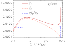
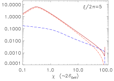
Figure 1: Distribution functions of electrons and positrons, $f_{e,p}(\chi)$, and a spectrum of emission, $\chi_{\gamma}f_{\gamma}(\chi)/\chi_{0}$, after the interaction of 46.6 GeV electrons with one cycle (left panel) and five cycles (right panel) of a laser pulse of intensity $J\approx 5\cdot 10^{22}\,{\rm W/cm}^{2}$ (so that $\chi\approx 2{\cal E}[GeV]$ — see Eq.(2)). Here $f_{e}-f_{p}$ is the distribution of the beam electrons and $\int{(f_{e}-f_{p})d\chi=1}$.

In Fig.1 the beam-wave interaction is traced during $\frac{\xi}{2\pi}=5$ cycles of the incident laser pulse ($\approx 13$ fs). The initial beam electron energy is rapidly converted into $\gamma$-photons with high $\chi_{\gamma}$, which then rapidly produce pairs, the typical rates of the processes being of the order of the inverse light period. However, the larger fraction of the new particles is born at $\chi\leq 1$, with strongly reduced pair production rate. Slow absorption of photons with $\chi_{\gamma}\sim 1-2$ maintains pair production even after tens of wave periods, as shown in Fig.2.

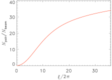
Figure 2: Pair production for longer pulse durations, measured in cycles. Other parameters are the same as in Fig.1.

V Conclusion

We see that the laser-beam interaction may be accompanied by multiple pair production. The initial energy of a beam electron is efficiently spent for creating pairs with significantly lower energies as well as softer $\gamma$-photons. This effect may be used for producing a pair plasma. It could also be employed to deactivation after-use electron beams, reducing radiation hazard.

The way to solve the kinetic equations is accurate and it does not employ the Monte-Carlo method. The solution can be used to benchmark numerical methods designed to simulate processes in QED-strong laser fields.

We acknowledge help and advice we received from S. S. Bulanov, M. Hegelich, J. G. Kirk, H. Ruhl, T. Schlegel and T. Tajima. One of us (I.S.) is supported by the DOE NNSA under the Predictive Science Academic Alliances Program by grant DE-FC52-08NA28616.

VI Appendix A. Electron in the QED-strong field: emission probability

In weaker fields, especially for the particular case of a harmonic wave, the emitted power is given by an integral over many periods of the wave. In this case, the solution of the emission problem in the weak harmonic wave field (under the requirement on the wave amplitude opposite to that formulated in Ineq.(1)) is given in Section 101 of lp as a sum over multi-photon-orders, resulting from the Fourier-series expansion for the (infinitely long) periodic wave. This standard approach, however, may become meaningless as applied to ultra-strong laser pulses, for many reasons. These pulses may be so short that they cannot be thought of as harmonic waves. Their fields may be strong enough to force an electron to expend its energy on radiation in less than a single wave period. However, an even more important point is that the radiation loss rate and even the spectrum of radiation is no longer an integral characteristic of the particle motion through a number of wave periods: a local dependence of emission on both particle and field characteristics is typical for the strong fields. The latter statement may be found in lp , Section 101. For the particular case of the 1D wave field the evaluation of the formation time for emission is provided in pre within the framework of classical electrodynamics. It is shown that the formation time is much shorter than the wave period as long as Ineq.(1) is fulfilled.

Here the emission problem is discused for QED-strong fields. We consider a 1D wave field taken in the Lorenz gauge okun :

$$a^{\mu}=a^{\mu}(\xi),\qquad\xi=(k\cdot x),\qquad(k\cdot a)=0,$$

$a^{\mu}=(0,{\bf a})$, $k^{\mu}$ and $x^{\mu}$ being the 4-vectors of the potential, the wave and the coordinates. Herewith the 4-dot-product is introduced in a usual manner: $(k\cdot x)=k^{\mu}x_{\mu}=\omega t-({\bf k}\cdot{\bf x})$ etc. Space-like 3-vectors (i.e., the first to the third components of a 4-vector) in contrast with 4-vectors are denoted in bold, 4-indices are denoted with Greek letters. Recall, that a metric signature $(+,-,-,-)$ is used, therefore, for space-like vectors the 3D scalar product and 4-dot-product have opposite signs, particularly:

$$\left(\frac{d{\bf a}}{d\xi}\right)^{2}=-\left(\frac{da}{d\xi}\right)^{2}\geq 0.$$

VI.1 Transformed space-time

A method facilitating many derivations involves the introduction of a specific time-space coordinate frame. Introduce a Transformed Space-Time (TST) :

$$x^{0,1}=(ct\mp x_{\|})/\sqrt{2},\qquad x^{2,3}={\bf x}_{\perp},$$

subscript $\perp$ denoting the vector components orthogonal to ${\bf k}$. The properties of the TST provide a convenient description for the classical motion of an electron in the 1D wave field. Note first that

$$dx^{0}=\frac{\lambdabar d\xi}{\sqrt{2}},\qquad p^{0}=\frac{\lambdabar(k\cdot p)}{\sqrt{2}},\qquad(p\cdot k)=\frac{{\cal E}-p_{\|}}{\lambdabar}.$$

Second, the generalized momentum components, $p^{0}$ and ${\bf p}_{\perp 0}={\bf p}_{\perp}+{\bf a}$, are conserved. Third, the metric tensor in the TST is:

$$G^{01}=G^{10}=1,\qquad G^{22}=G^{33}=-1,\qquad G^{\mu\nu}=G_{\mu\nu}.$$

Note the unusual off-diagonal structure of the metric tensor, resulting in a strange relationship between contravariant and covariant coordinates: $x^{0}=x_{1}$, $x^{1}=x_{0}$. Specifically, the (contravariant) component of the electron momentum, $p^{0}$, is a motional invariant, as long as the vector-potential (and the Hamiltonian, $H$) does not depend on the (covariant) coordinate, $x_{0}$ (despite its dependence on $x^{0}$):

$$\frac{dp^{0}}{dt}\propto-\frac{\partial H}{\partial x_{0}}=0.$$

Finally, the identity, ${\cal E}^{2}=p^{2}+1$, being expanded in the TST metric, gives:

$$p^{1}=\frac{1+{\bf p}_{\perp}^{2}}{2p^{0}}=\frac{1+({\bf p}_{\perp 0}-{\bf a})^{2}}{\sqrt{2}\lambdabar(k\cdot p)}.$$

The derivative over $x^{0}$ or, the same, over $\xi$ is conveniently related to the derivative over the proper time for electron:

$$\frac{d}{d\tau}={\cal E}\left[\frac{\partial}{\partial t}+({\bf v}\cdot\frac{\partial}{\partial{\bf x}})\right]=c(k\cdot p)\frac{d}{d\xi}.$$ (16)

VI.2 Classical trajectory and momenta retarded product

Many characteristics of emission may be expressed in terms of the relationship between the 4-momenta of the electron at different instants:

$$p^{\mu}(\xi)=p^{\mu}(\xi_{1})-\delta a^{\mu}+\frac{2(p(\xi_{1})\cdot\delta a)-(\delta a)^{2}}{2(k\cdot p)}k^{\mu},$$ (17)

where

$$\delta a^{\mu}=a^{\mu}(\xi)-a^{\mu}(\xi_{1}).$$

As a consequence from Eq.(17), one can obtain the expression for the Momenta Retarded Product (MRP):

$$(p(\xi)\cdot p(\xi_{1}))=1-\frac{(\delta a)^{2}}{2}=1+\frac{(\delta{\bf a})^{2}}{2},$$ (18)

Note, that the MRP is given by Eq.(18) for an arbitrary difference between $\xi$ and $\xi_{1}$, but only for the particular case of the 1D wave field. However the limit of this formula as $|\xi-\xi_{1}|\rightarrow 0$, which is as follows:

$$(p(\xi)\cdot p(\xi_{1}))|_{|\xi-\xi_{1}|\rightarrow 0}\approx 1+\frac{1}{2}(\xi-\xi_{1})^{2}\left|\frac{d{\bf a}}{d\xi}\right|^{2}$$

or, in terms of the MRP in the proper time, $\tau$:

$$(p(\tau)\cdot p(\tau+\delta\tau))=1-(\delta\tau)^{2}\frac{(f\cdot f)}{2m_{e}^{2}c^{2}},$$ (19)

has a much wider range of applicability. Eq.(19) is derived from the equation of motion:

$$\frac{dp^{\mu}}{d\tau}=\frac{f^{\mu}}{m_{e}c},$$

using the identities:

$$(p(\tau)\cdot p(\tau))=1,\qquad(p(\tau)\cdot f(\tau))=0,$$

$$\frac{d(p(\tau)\cdot p(\tau+\delta\tau))}{d(\delta\tau)}=-\delta\tau\left(\frac{dp}{d\tau}\cdot\frac{dp}{d\tau}\right)+O((\delta\tau)^{2}).$$

Here $f^{\mu}$ is the Lorentz four-force:

$$f^{\mu}=(f^{0},{\bf f}^{(3)}),\qquad f^{0}=e{\bf E}\cdot{\bf p},\qquad{\bf f}^{(3)}=e{\cal E}{\bf E}+e{\bf p}\times{\bf B}.$$

VI.3 A solution of the Dirac equation

The Dirac equation which determines the evolution of the wave function, $\psi$, for a non-emitting electron in the external field, reads:

$$\left[i\lambdabar_{C}\left(\gamma\cdot\frac{\partial}{\partial x}\right)-(\gamma\cdot a)\right]\psi=\psi,$$ (20)

$\gamma^{\mu}$ being the Dirac $4*4$ matrices, $(\gamma^{0},\gamma^{1},\gamma^{2},\gamma^{3})$. The relativistic dot-product of the Dirac matrices by 4-vector, such as $(\gamma\cdot a)$, is the linear combination of the Dirac matrices: $(\gamma\cdot a)=\gamma^{0}a^{0}-\gamma^{1}a^{1}-\gamma^{2}a^{2}-\gamma^{3}a^{3}$. Such a linear combination, which is also a $4*4$ matrix, may be multiplied by another matrix of this kind or by 4-component bi-spinor, such as $\psi$, following matrix multiplication rules. For example, $(\gamma\cdot a)\psi$ is a bi-spinor, as is the matrix, $(\gamma\cdot a)$ multiplied from the right hand side by the bi-spinor, $\psi$.

The solution of Eq.(20) in a form of a plane electron wave can be conveniently expressed in terms of the classical solution:

$$\psi=\frac{1}{\sqrt{N}}u(p(\xi))\exp(-i\int^{x}{\left((p(\xi)+eA)\cdot dx\right)}),$$ (21)

the normalization coefficient $N={\rm const}$. By expanding the phase multiplier in the TST, a more convenient form can be provided:

$$\psi=\frac{u(p(\xi))P(\xi)}{\sqrt{N}}\exp\left[\frac{i\left[({\bf p}_{\perp 0}\cdot{\bf x}_{\perp})-\frac{\lambdabar(k\cdot p)x^{1}}{\sqrt{2}}\right]}{\lambdabar_{C}}\right].$$ (22)

Here $u(p(\xi))$ is plane wave bi-spinor amplitude, which satisfies the system of four linear algebraic equations:

$$(\gamma\cdot p(\xi))u(p(\xi))=u(p(\xi)),$$ (23)

as well as the normalization condition: $\hat{u}u=2.$ The $\xi$-dependent phase multiplier, $P(\xi)$, is as follows:

$$P(\xi)=\exp\left(-\frac{i}{\lambdabar_{C}}\int^{\xi}{\frac{1+{\bf p}_{\perp}^{2}(\xi_{2})}{2(k\cdot p)}d\xi_{2}}\right),$$

or,

$$P(\xi)=P(\xi_{1})\exp\left(-\frac{i}{\lambdabar_{C}}\int^{\xi}_{\xi_{1}}{\frac{1+{\bf p}_{\perp}^{2}(\xi_{2})}{2(k\cdot p)}d\xi_{2}}\right).$$ (24)

Using Eq.(17), one can find:

$$u(p(\xi))=\left[1+\frac{(\gamma\cdot k)\left(\gamma\cdot[a(\xi)-a(\xi_{1})]\right)}{2(k\cdot p)}\right]u(p(\xi_{1}))$$ (25)

and verify that Eq.(22) satisfies the Dirac equation. To prove all these assertions, note that the plane wave bi-spinor amplitude once expressed in terms of the classical solution Eq.(17), satisfies the following commutation rule:

$$\left[(\gamma\cdot p(\xi))\pm 1\right]\left[1+\frac{(\gamma\cdot k)}{2(k\cdot p)}(\gamma\cdot\delta a)\right]=\left[1+\frac{(\gamma\cdot k)}{2(k\cdot p)}(\gamma\cdot\delta a)\right]\left[(\gamma\cdot p(\xi_{1}))\pm 1\right].$$ (26)

The latter can be proved using the commutation rules as in Eqs.(22.5) from lp for the Dirac matrices as well as the identities, $(k\cdot A)=(k\cdot k)=0$:

$$\left[(\gamma\cdot p(\xi_{1}))-(\gamma\cdot\delta a)+\frac{2(p(\xi_{1})\cdot\delta a)-(\delta a)^{2}}{2(k\cdot p)}(\gamma\cdot k)\pm 1\right]\left[1+\frac{(\gamma\cdot k)(\gamma\cdot\delta a)}{2(k\cdot p)}\right]=$$

$$(\gamma\cdot p(\xi_{1}))-(\gamma\cdot\delta a)+\frac{2(p(\xi_{1})\cdot\delta a)-(\gamma\cdot p(\xi_{1}))(\gamma\cdot\delta a)}{2(k\cdot p)}(\gamma\cdot k)\pm\left[1+\frac{(\gamma\cdot k)(\gamma\cdot\delta a)}{2(k\cdot p)}\right]=$$

$$=\left[1+\frac{(\gamma\cdot k)(\gamma\cdot\delta a)}{2(k\cdot p)}\right]\left[(\gamma\cdot p(\xi_{1}))\pm 1\right].$$

Thus, Eq.(26) is proved. This commutation rule allows us to verify that $u(p(\xi))$ is indeed a bi-spinor amplitude of a planar wave with the four-vector $p(\xi)$, satisfying Eq.(23). Finally, to verify that Eq.(22) gives the solution of the Dirac equation, one should account for Eq.(23) as well as the identity,

$$(\gamma\cdot k)\frac{d[u(p(\xi))]}{d\xi}=(\gamma\cdot k)(\gamma\cdot k)\left(\gamma\cdot\frac{dA}{d\xi}\right)u(p_{0})=0,$$

which is valid, because $(\gamma\cdot k)(\gamma\cdot k)=k^{2}=0$,

The advantage of the approach used here as compared to the known Volkov solution (see Section 40 in lp ) is that the wave function in Eqs.(22-25) is described in a self-contained manner within some finite time interval, $(\xi_{1},\xi)$ (in fact, this interval is assumed to be very short below) in terms of the local parameters of the classical trajectory of electrons. This approach is better applicable to strong fields, in which the time interval between subsequent emission occurrences, which destroys the unperturbed wave function, becomes very short.

VI.4 The matrix element for emission

The emission problem is formulated in the following way. The electron motion in the strong field may be thought of as a sequence of short intervals. Within each of these intervals the electron follows a piece of a classical trajectory, as in Eq.(17), and its wave function (an electron state) is given by Eq.(22). The transition from one piece of the classical trajectory to another, or, the same, from one electron state to another occurs in a probabilistic manner. The probability of this transition, which is accompanied by a photon emission is calculated below using the QED perturbation theory. We consider the laser wave field as a classical field ($\lambdabar_{C}(k\cdot p)\ll 1$) and apply first-order perturbation theory with respect to the Hamiltonian of the electron-photon interaction, $\hat{H}\propto(\hat{j}\cdot\hat{A})$.

The only difficulty specific to strong pulsed fields is that the short piece of the electron trajectory is strictly bounded in space and in time, while the QED invariant perturbation theory is based on the ’matrix element’, which is the integral over infinite 4-volume.

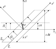
Figure 3: The volume over which to integrate the matrix element while finding the emission probability: in the standard scheme for the dipole emission (in dashed lines) and in the TST (in solid lines). Arrows show the direction, along which the Heisenberg operator advances the wave functions.

To avoid this difficulty the following method is suggested, which is analogous to the dipole emission theory as applied in TST. Introduce domain, $\Delta^{4}x=(\Delta x^{1}*S_{\perp})*\Delta x^{0}$, bounded by two hypersurfaces, $\xi=\xi_{-}$ and $\xi=\xi_{+}$ (see Fig.3). The difference $\xi_{+}-\xi_{-}$ is bounded as described below, so that $\Delta^{4}x$ covers only a minor part of the pulse. A volume,

$$V=S_{\perp}\lambdabar(\xi_{+}-\xi_{-})=S_{\perp}\lambdabar\int_{\xi_{-}}^{\xi_{+}}{d\xi_{2}},$$

is a section of $\Delta^{4}x$ subtended by a line $t={\rm const}$.

With the following choice for the normalization coefficient in Eq.(22):

$$N=2S_{\perp}\lambdabar\int_{\xi_{-}}^{\xi_{+}}{{\cal E}(\xi_{2})d\xi_{2}},$$

the integral of the electron density in the volume $V$

$$\int{\hat{\psi}\gamma^{0}\psi dV}=S_{\perp}\lambdabar\int_{\xi_{-}}^{\xi_{+}}{\hat{\psi}\gamma^{0}\psi d\xi_{2}},$$

is set to unity, i.e. there is a single electron in the volume $V$. This statement follows from Eq.(22) and the known property of normalized bi-spinor amplitudes: $\hat{u}\cdot\gamma^{0}\cdot u=2{\cal E}$. Here the hat means the Dirac conjugation.

For a photon of wave vector, $(k^{\prime})^{\mu}$, and polarization vector, $l^{\mu}$, introduce the wave function:

$$(A^{\prime})^{\mu}=\frac{\exp[-i(k^{\prime}\cdot x)/\lambdabar_{C}]}{\sqrt{N_{p}}}l^{\mu},$$

or, by expanding this in the TST:

$$(A^{\prime})^{\mu}=\frac{P_{p}(\xi)}{\sqrt{N_{p}}}\exp\left[\frac{i({\bf k}^{\prime}_{\perp}\cdot{\bf x}_{\perp})}{\lambdabar_{C}}-\frac{i\lambdabar(k\cdot k^{\prime})x^{1}}{\sqrt{2}\lambdabar_{C}}\right]l^{\mu},$$

where:

$$P_{p}(\xi)=\exp\left[-i\xi\frac{({\bf k}^{\prime}_{\perp})^{2}}{2(k\cdot k^{\prime})\lambdabar_{C}}\right].$$

Here the photon momentum and photon energy are related to $m_{e}c$ and $m_{e}c^{2}$ correspondingly, or, equivalently, dimensionless $(k^{\prime})^{\mu}$ equals dimensional $(k^{\prime})^{\mu}$ multiplied by $\lambdabar_{C}$. The choice of the normalization coefficient,

$$N_{p}=\frac{\omega^{\prime}V}{2\pi\hbar c\lambdabar_{C}},$$

corresponds to a single photon in the volume, $V$.

The emission probability, $dW$, is given by an integral over $\Delta^{4}x$:

$$dW=\frac{\alpha L_{f}L_{p}}{\hbar c}\left|\int{\hat{\psi}_{f}(\gamma\cdot(A^{\prime})^{*})\psi_{i}dx^{0}dx^{1}dx^{2}dx^{3}}\right|^{2}.$$ (27)

Here

$$L_{p}=\frac{Vd^{3}{\bf k}^{\prime}}{(2\pi\lambdabar_{C})^{3}}=\frac{\hbar cN_{p}d^{2}{\bf k}^{\prime}_{\perp}d(k\cdot k^{\prime})}{(2\pi\lambdabar_{C})^{2}(k\cdot k^{\prime})}$$ (28)

is the number of states for the emitted photon. The transformation of the phase volume as in Eq.(28) is based on the following Jacobian:

$$\left(\frac{\partial k^{\prime}_{\|}}{\partial(k^{\prime}\cdot k)}\right)_{{\bf k}^{\prime}_{\perp}={\rm const}}=\frac{\omega^{\prime}}{(k^{\prime}\cdot k)},$$

which is also used below in many places. A subscript $i,f$ denotes the electron in the initial (i) or final (f) state. The number of electron states in the presence of the wave field, $L_{i,f}$, should be integrated over the volume $V$

$$L_{i,f}=\frac{1}{(2\pi\lambdabar_{C})^{3}}\int_{V}{d^{3}{\bf p}_{i,f}dV}=\frac{d(k\cdot p)_{i,f}d^{2}{\bf p}_{\perp i,f}N_{i,f}}{2(2\pi)^{3}\lambdabar_{C}^{3}(k\cdot p)_{i,f}}.$$

VI.5 Conservation laws

The integration by $dx^{1}dx^{2}dx^{3}=c\sqrt{2}dtd^{2}{\bf x}_{\perp}$ results in three $\delta-$ functions, expressing the conservation of totals of ${\bf p}_{\perp}$ and $(k\cdot p)$, for particles in initial and final states:

$${\bf p}_{\perp i}={\bf p}_{\perp f}+{\bf k}_{\perp}^{\prime},\qquad(k\cdot p_{i})=(k\cdot p_{f})+(k\cdot k^{\prime}).$$

Twice integrated with respect to $dx^{1}$, the probability $dW$ is proportional to a long time interval, $\Delta t=\Delta x^{1}/(c\sqrt{2})$, if the boundary condition for the electron wave at $\xi=\xi_{-}$ is maintained within that long time. On transforming the integral over $dx^{0}$ to that over $d\xi$, one can find:

$$\left|\int{...d^{4}x}\right|^{2}=(2\pi\lambdabar_{C})^{3}S_{\perp}c\Delta t\lambdabar\left|\int{...d\xi}\right|^{2}\times$$

$$\times\delta^{2}({\bf p}_{\perp i}-{\bf p}_{\perp f}-{\bf k}_{\perp}^{\prime})\delta((k\cdot p_{i})-(k\cdot p_{f})-(k\cdot k^{\prime})).$$

To take the large value of $\Delta t$ seems to be the only way to calculate the integral, however, the emission probability calculated in this way relates to multiple electrons in the initial state, each of them locating between the wave fronts $\xi=\xi_{-}$ and $\xi=\xi_{+}$ during much shorter time,

$$\delta t(\xi_{-},\xi_{+})=(1/c)\int_{\xi_{-}}^{\xi^{+}}{{\cal E}_{i}(\xi)d\xi_{2}}/(k\cdot p_{i}).$$ (29)

For a single electron the emission probability becomes:

$$dW_{fi}(\xi_{-},\xi_{+})=\delta tdW/\Delta t.$$

Using $\delta-$ functions it is easy to integrate Eq.(27) over $d{\bf p}_{\perp f}d(k\cdot p_{f})$:

$$\frac{dW_{fi}(\xi_{-},\xi_{+})}{d(k\cdot k^{\prime})d^{2}{\bf k}^{\prime}_{\perp}}=\frac{\alpha\left|\int_{\xi_{-}}^{\xi_{+}}{T(\xi)\hat{u}(p_{f})(\gamma\cdot l^{*})u(p_{i})d\xi}\right|^{2}}{(4\pi\lambdabar_{C})^{2}(k\cdot k^{\prime})(k\cdot p_{i})(k\cdot p_{f})},$$

where

$$T(\xi)=\frac{P_{i}(\xi)}{P_{f}(\xi)P_{p}(\xi)}=\exp\left[\frac{i\int^{\xi}{(k^{\prime}\cdot p_{i,f}(\xi_{2}))d\xi_{2}}}{\lambdabar_{C}(k\cdot p_{f,i})}\right],$$

$P_{i}(\xi)$ and $P_{f}(\xi)$ are the electron phase multipliers, $P(\xi)$, for the electron in initial and final states and

$$p^{\mu}_{f}(\xi)=p^{\mu}_{i}(\xi)-(k^{\prime})^{\mu}+\frac{(k^{\prime}\cdot p_{i}(\xi))}{(k\cdot p_{i})-(k\cdot k^{\prime})}k^{\mu}.$$ (30)

If in the expression for $T(\xi)$ the numerator of the fraction is taken for the initial state of electron, then the denominator should be taken for the final state and vise versa.

Prior to discussing Eq.(30), return to Eq.(17) and analyze it component-by-component in the TST. It appears that three of the four components of that equation describe the conservation of $(k\cdot p)$ and ${\bf p}_{\perp 0}={\bf p}_{\perp}+{\bf a}$ for electron in the course of its emission-free motion. At the same time, yet another component of Eq.(17), specifically, $p^{1}$, directed along $k^{\mu}$, describes the energy-momentum exchange between the electron and the 1D wave field, maintaining the identity, $(p\cdot p)=1$. Now turn to Eq.(30). Again, three of the four components express the conservation of the same variables in the course of the photon emission, while the $p^{1}$ component, directed along $k^{\mu}$ describes the absorption of energy and momentum from the wave field in the course of the photon emission. Note, that in the case of a strong field, the energy absorbed from field is not an integer number of quanta, and that for short non-harmonic field it is not even a constant, but a function of the local field.

VI.6 Calculation of the matrix element: a product of the Dirac matrices

To calculate the matrix element, one can re-write it as the double integral over $d\xi d\xi_{1}$. The integrand in this double integral includes the phase multiplier and the following matrix product:

$$\hat{u}(p_{f}(\xi))(\gamma\cdot l^{*})u(p_{i}(\xi))\left[\hat{u}(p_{f}(\xi_{1}))(\gamma\cdot l^{*})u(p_{i}(\xi_{1}))\right]^{*}=...$$ (31)

Using Eq.(25) one can reduce the multipliers of the kind of $u(p_{i}(\xi))\otimes\hat{u}(p_{i}(\xi_{1}))$ to $u(p_{i}(\xi_{1}))\otimes\hat{u}(p_{i}(\xi_{1}))$, which can be expressed in terms of the polarization density matrix at the position $\xi_{1}$. Although in a strong wave electrons may be polarized (see Omori ), in the present work the emission probability is assumed to be averaged over the electron initial and final polarizations. Therefore, the polarization matrix is used in the form of $1/2[(\gamma\cdot p_{i}(\xi))+1]$ and one can re-write the integrand as follows:

$$...=\frac{1}{4}{\rm Sp}\{\left[1+\frac{(\gamma\cdot k)}{2(k\cdot p_{f})}(\gamma\cdot[a(\xi_{1})-a(\xi)])\right]\times$$

$$\times\left[(\gamma\cdot p_{f}(\xi))+1\right](\gamma\cdot l^{*})\times\\ \left[1+\frac{(\gamma\cdot k)}{2(k\cdot p_{i})}(\gamma\cdot[a(\xi)-a(\xi_{1})])\right]\left[(\gamma\cdot p_{i}(\xi_{1}))+1\right](\gamma\cdot l)\}=...$$

In transforming the trace of matrix in addition to the mentioned above relationships and the Dirac matrix algebra we use the commutation rule Eq.(26), the conservation law Eq.(30), and the identity $(l^{*}\cdot l)=-1$ for a spatial unity vector of the emitted photon polarization, which can be also written as $(\gamma\cdot l^{*})(\gamma\cdot p_{i,f})(\gamma\cdot l)=2(l^{*}\cdot p_{i,f})(\gamma\cdot l)+(\gamma\cdot p_{i,f})$. Move $(\gamma\cdot p_{f}(\xi)+1)$ to the first position using the commutation rule Eq.(26) and then move it to the last position. In the product $[(\gamma\cdot p_{i}(\xi_{1}))+1](\gamma\cdot l)[(\gamma\cdot p_{f}(\xi_{1}))+1]$ we should keep only odd powers in $\gamma$, as long as in the preceding multiplier only odd powers of $\gamma$ are present:

$$...=\frac{1}{4}{\rm Sp}\{\left[1+\frac{(\gamma\cdot k)}{2(k\cdot p_{f})}(\gamma\cdot[a(\xi_{1})-a(\xi)])\right](\gamma\cdot l^{*})\times$$

$$\left[1+\frac{(\gamma\cdot k)}{2(k\cdot p_{i})}(\gamma\cdot[a(\xi)-a(\xi_{1})])\right]\left[(\gamma\cdot p_{i}(\xi_{1}))(\gamma\cdot l)(\gamma\cdot p_{f}(\xi_{1}))+(\gamma\cdot l)\right]\}=$$

In the product of the first three multipliers separate the even powers in $a$, which are $(\gamma\cdot l^{*})-(\gamma\cdot k)(l^{*}\cdot k)(a(\xi)-a(\xi_{1}))^{2}/[2(k\cdot p_{i})(k\cdot p_{f})]$. The traces of the products of two or four Dirac matrices are calculated using Eqs.(22.9-10) from lp .

$$=\left[(p_{i}(\xi_{1})\cdot p_{f}(\xi_{1}))-1\right]\left[1+\frac{(l^{*}\cdot k)(l\cdot k)}{2(k\cdot p_{i})(k\cdot p_{f})}(a(\xi)-a(\xi_{1}))^{2}\right]+(l^{*}\cdot p_{i}(\xi_{1}))(l\cdot p_{f}(\xi_{1}))+$$

$$+(l\cdot p_{i}(\xi_{1}))(l^{*}\cdot p_{f}(\xi_{1}))-\left[\frac{(l^{*}\cdot k)(l\cdot p_{i}(\xi_{1}))}{2(k\cdot p_{i})}+\frac{(l^{*}\cdot k)(l\cdot p_{f}(\xi_{1}))}{2(k\cdot p_{f})}\right](a(\xi)-a(\xi_{1}))^{2}+$$

In one of the two terms linear in $a$ we move $(\gamma\cdot l^{*})$ from the first to the last position:

$$+\frac{1}{8(k\cdot p_{i})}{\rm Sp}\left\{(\gamma\cdot k)(\gamma\cdot[a(\xi)-a(\xi_{1})])(\gamma\cdot p_{i}(\xi_{1}))[2(l^{*}\cdot p_{f}(\xi_{1}))(\gamma\cdot l)+(\gamma\cdot p_{f}(\xi_{1}))]\right\}-$$

$$-\frac{1}{8(k\cdot p_{f})}{\rm Sp}\left\{(\gamma\cdot k)(\gamma\cdot[a(\xi)-a(\xi_{1})])[2(l^{*}\cdot p_{i}(\xi_{1}))(\gamma\cdot l)+(\gamma\cdot p_{i}(\xi_{1}))](\gamma\cdot p_{f}(\xi_{1}))\right\}=$$

Calculate traces for the products of four Dirac matrices in the terms linear in $a$:

$$=\left[(p_{i}(\xi_{1})\cdot p_{f}(\xi_{1}))-1\right]\left[1+\frac{(l^{*}\cdot k)(l\cdot k)}{2(k\cdot p_{i})(k\cdot p_{f})}(a(\xi)-a(\xi_{1}))^{2}\right]+(l^{*}\cdot p_{i}(\xi_{1}))(l\cdot p_{f}(\xi_{1}))+$$

$$+(l\cdot p_{i}(\xi_{1}))(l^{*}\cdot p_{f}(\xi_{1}))-\left[\frac{(l^{*}\cdot k)(l\cdot p_{i}(\xi_{1}))}{2(k\cdot p_{i})}+\frac{(l^{*}\cdot k)(l\cdot p_{f}(\xi_{1}))}{2(k\cdot p_{f})}\right](a(\xi)-a(\xi_{1}))^{2}+$$

$$+\{-\frac{1}{2}(\left[a(\xi)-a(\xi_{1})\right]\cdot p_{i}(\xi_{1}))+$$

$$+\frac{(k\cdot p_{i})}{2(k\cdot p_{f})}(\left[a(\xi)-a(\xi_{1})\right]\cdot p_{f}(\xi_{1}))-\frac{1}{2}(\left[a(\xi)-a(\xi_{1})\right]\cdot p_{f}(\xi_{1}))+\frac{(k\cdot p_{f})}{2(k\cdot p_{i})}(\left[a(\xi)-a(\xi_{1})\right]\cdot p_{i}(\xi_{1}))-$$

$$-\left(\left[p_{f}(\xi_{1})+p_{i}(\xi_{1})\right]\cdot l^{*}\right)\left(l\cdot\left[a(\xi)-a(\xi_{1})\right]\right)+\frac{([a(\xi)-a(\xi_{1})]\cdot p_{i}(\xi_{1}))(k\cdot l)(l^{*}\cdot p_{f}(\xi_{1}))}{(k\cdot p_{i})}+$$

$$\frac{([a(\xi)-a(\xi_{1})]\cdot p_{f}(\xi_{1}))(k\cdot l)(l^{*}\cdot p_{i}(\xi_{1}))}{(k\cdot p_{f})}\}=$$

Group the terms proportional to $(l^{*}\cdot p_{i,f}(\xi_{1}))$

$$=(l^{*}\cdot p_{i}(\xi_{1}))\left(l\cdot\left\{p_{f}(\xi_{1})-\left[a(\xi)-a(\xi_{1})\right]+k\frac{([a(\xi)-a(\xi_{1})]\cdot p_{f}(\xi_{1}))}{(k\cdot p_{f})}\right\}\right)+$$

$$+(l^{*}\cdot p_{f}(\xi_{1}))\left(l\cdot\left\{p_{i}(\xi_{1})-\left[a(\xi)-a(\xi_{1})\right]+k\frac{([a(\xi)-a(\xi_{1})]\cdot p_{i}(\xi_{1}))}{(k\cdot p_{i})}\right\}\right)+$$

Group in an analogous manner the terms, proportional to $(p_{i,f}(\xi_{1})\cdot...)$:

$$+\frac{1}{2}\left(p_{i}(\xi_{1})\cdot\left\{p_{f}(\xi_{1})-\left[a(\xi)-a(\xi_{1})\right]+k\frac{([a(\xi)-a(\xi_{1})]\cdot p_{f}(\xi_{1}))}{(k\cdot p_{f})}\right\}\right)+$$

$$+\frac{1}{2}\left(p_{f}(\xi_{1})\cdot\left\{p_{i}(\xi_{1})-\left[a(\xi)-a(\xi_{1})\right]+k\frac{([a(\xi)-a(\xi_{1})]\cdot p_{i}(\xi_{1}))}{(k\cdot p_{i})}\right\}\right)-1+$$

The residual terms are $\propto(\delta a)^{2}$:

$$+\left\{\left[(p_{i}(\xi_{1})\cdot p_{f}(\xi_{1}))-1\right](l^{*}\cdot k)(l\cdot k)-(l^{*}\cdot k)(l\cdot p_{i}(\xi_{1}))(k\cdot p_{f})-(l^{*}\cdot k)(l\cdot p_{f}(\xi_{1}))(k\cdot p_{i})\right\}\times$$

$$\times\frac{(a(\xi)-a(\xi_{1}))^{2}}{2(k\cdot p_{i})(k\cdot p_{f})}=$$

Use Eq.(30) and introduce wherever reasonable the functions of $\xi$:

$$=(l^{*}\cdot p_{i}(\xi_{1}))\left(l\cdot p_{f}(\xi)\right)+(l^{*}\cdot p_{f}(\xi_{1}))\left(l\cdot p_{i}(\xi)\right)+$$

$$+(l^{*}\cdot p_{i}(\xi_{1}))\left(l\cdot k\right)\frac{\left[a(\xi)-a(\xi_{1})\right]^{2}}{2(k\cdot p_{f})}+(l^{*}\cdot p_{f}(\xi_{1}))\left(l\cdot k\right)\frac{\left[a(\xi)-a(\xi_{1})\right]^{2}}{2(k\cdot p_{i})}+$$

$$+\left\{\left[(p_{i}(\xi_{1})\cdot p_{f}(\xi_{1}))-1\right](l^{*}\cdot k)(l\cdot k)-(l^{*}\cdot k)(l\cdot p_{i}(\xi_{1}))(k\cdot p_{f})-(l^{*}\cdot k)(l\cdot p_{f}(\xi_{1}))(k\cdot p_{i})\right\}\times$$

$$\times\frac{(a(\xi)-a(\xi_{1}))^{2}}{2(k\cdot p_{i})(k\cdot p_{f})}+$$

The total of all terms proportional to $(a(\xi)-a(\xi_{1}))^{2}$ given above vanishes. This can be shown using the following properties: the tensor $l\otimes l^{*}$ is Hermitian; the difference $p_{f}-p_{i}$ is the total of two terms, proportional to $k$ and $k^{\prime}$, the latter being orthogonal to $l$. The residual terms are:

$$+\frac{1}{2}\left(p_{i}(\xi_{1})\cdot\left\{p_{f}(\xi)+k\frac{\left[a(\xi)-a(\xi_{1})\right]^{2}}{2(k\cdot p_{f})}\right\}\right)+$$

$$+\frac{1}{2}\left(p_{f}(\xi_{1})\cdot\left\{p_{i}(\xi)+k\frac{\left[a(\xi)-a(\xi_{1})\right]^{2}}{2(k\cdot p_{i})}\right\}\right)-$$

The last term, $-1$, we transform using Eq.(18)

$$-\frac{1}{2}\left[a(\xi)-a(\xi_{1})\right]^{2}-\frac{1}{2}(p_{i}(\xi)\cdot p_{i}(\xi_{1}))-\frac{1}{2}(p_{f}(\xi)\cdot p_{f}(\xi_{1}))=$$

$$=(l^{*}\cdot p_{i}(\xi_{1}))\left(l\cdot p_{f}(\xi)\right)+(l^{*}\cdot p_{f}(\xi_{1}))\left(l\cdot p_{i}(\xi)\right)-\left(\left[p_{f}(\xi)-p_{i}(\xi)\right]\cdot\left[p_{f}(\xi_{1})-p_{i}(\xi_{1})\right]\right)+$$

$$+\frac{\left[a(\xi)-a(\xi_{1})\right]^{2}\left((k\cdot p_{i})-(k\cdot p_{f})\right)^{2}}{4(k\cdot p_{i})(k\cdot p_{f})}.$$

On substituting this into the integral expression for the matrix element, some terms give zero contributions to the integral. Particularly, the following integrals vanish, as long as the expressions in the square brackets are the perfect time derivatives:

$$\int{\left[(k^{\prime}\cdot p_{i,f}(\xi))\exp(\int^{\xi}{\frac{(k^{\prime}\cdot p_{i,f}(\xi_{1}))}{(k\cdot p_{f,i})}d\xi_{2}})\right]d\xi}=0.$$

From here it is also easy to derive that:

$$\int{\left[(p_{i}(\xi)-p_{f}(\xi)-k^{\prime})\exp(\int^{\xi}{\frac{(k^{\prime}\cdot p_{i,f}(\xi_{1}))}{(k\cdot p_{f,i})}d\xi_{2}})\right]d\xi}=0.$$

Therefore, with the transformed product of the Dirac matrices, which should be multiplied by a factor of two (as long as we should sum over the final electron polarization instead of averaging), we obtain:

$$\frac{dW_{fi}}{d(k\cdot k^{\prime})d^{2}{\bf k}^{\prime}_{\perp}}=\frac{\alpha\int_{\xi_{-}}^{\xi_{+}}{\int_{\xi_{-}}^{\xi_{+}}{T(\xi)T(-\xi_{1})]Dd\xi d\xi_{1}}}}{(2\pi\lambdabar_{C})^{2}(k\cdot k^{\prime})(k\cdot p_{i})(k\cdot p_{f})},$$ (32)

where

$$D=(l^{*}\cdot p_{i}(\xi_{1}))(l\cdot p_{i}(\xi))+\frac{\left[a(\xi)-a(\xi_{1})\right]^{2}\left((k\cdot p_{i})-(k\cdot p_{f})\right)^{2}}{8(k\cdot p_{i})(k\cdot p_{f})}.$$

The matrix element may also be summed, if desired, for two possible directions of the polarization vector. The second term in the integrand is simply multiplied by two, while in the first one the negative of the metric tensor should be substituted for the product of the polarization vectors (see Section 8 in lp ), so that $-\left(p_{i}(\xi)\cdot p_{i}(\xi_{1})\right)$ substitutes for $\sum_{l}{(l^{*}\cdot p_{i}(\xi_{1}))(l\cdot p_{i}(\xi))}$. The latter may be transformed using Eq.(18), thus, giving:

$$\sum_{l}{D}=-1+\frac{\left[a(\xi)-a(\xi_{1})\right]^{2}\left((k\cdot p_{i})^{2}+(k\cdot p_{f})^{2}\right)}{4(k\cdot p_{i})(k\cdot p_{f})}.$$

VI.7 Calculation of the matrix element: integration

Now perform integration over ${\bf k}_{\perp}$. On developing the dot-product, $(k^{\prime}\cdot p_{i})$, in $T(\xi)$ in the TST metric, $G^{\mu\nu}$, one can find:

$$T(\xi)T(-\xi_{1})=\exp\left[i(T_{1}+T_{2})\right],$$

where

$$T_{1}=\frac{(k\cdot p_{i})}{2\lambdabar_{C}(k\cdot k^{\prime})(k\cdot p_{f})}\left(\frac{(k\cdot k^{\prime})}{(k\cdot p_{i})}\left<{\bf p}_{\perp i}\right>-{\bf k}^{\prime}_{\perp}\right)^{2}(\xi-\xi_{1}),$$

$$T_{2}=\frac{(k\cdot k^{\prime})\left\{(\xi-\xi_{1})+\int_{\xi_{1}}^{\xi}{\left[{\bf a}(\xi_{2})-\left<{\bf a}\right>\right]^{2}d\xi_{2}}\right\}}{2\lambdabar_{C}(k\cdot p_{i})(k\cdot p_{f})},$$

$$\left<{\bf a}\right>=\frac{\int_{\xi_{1}}^{\xi}{{\bf a}d\xi_{2}}}{\xi-\xi_{1}},\qquad\left<{\bf p}_{\perp i}\right>={\bf p}_{\perp 0i}-\left<{\bf a}\right>.$$

Integration over $d^{2}{\bf k}^{\prime}_{\perp}$ is performed using the following formula:

$$\int{\exp\left(iT_{1}\right)d^{2}{\bf k}_{\perp}}=\pi\int_{0}^{\infty}{\exp\left(iT_{1}\right)d\left(\frac{(k\cdot k^{\prime})}{(k\cdot p_{i})}\left<{\bf p}_{\perp i}\right>-{\bf k}^{\prime}_{\perp}\right)^{2}}.$$

The right hand side is proportional to $\exp(iT_{1})_{|{\bf k}_{\perp}|\rightarrow\infty}-1$, where the rapidly oscillating at large $|{\bf k}_{\perp}|$ term results in a vanishing contribution to the integral over $d\xi d\xi_{1}$ and should be neglected. The integrated over ${\bf k}_{\perp}$ probability is:

$$\frac{dW_{fi}(\xi_{-},\xi_{+})}{d(k\cdot k^{\prime})}=\frac{\alpha\int_{\xi_{-}}^{\xi_{+}}{\int_{\xi_{-}}^{\xi_{+}}{\frac{i\exp(iT_{2})}{\xi-\xi_{1}}\sum_{l}{D(\xi,\xi_{1})}d\xi d\xi_{1}}}}{2\pi\lambdabar_{C}(k\cdot p_{i})^{2}}.$$

In strong fields the following estimates may be applied:

$$(k\cdot k^{\prime})\sim\lambdabar_{C}(k\cdot p_{i})^{2}\left|\frac{d{\bf a}}{d\xi}\right|,\qquad dW_{fi}\sim\alpha\left|(\xi_{+}-\xi_{-})\frac{d{\bf a}}{d\xi}\right|.$$

Now the bounds for $\xi_{+}-\xi_{-}$ can be consistently introduced:

$$\left|d{\bf a}/d\xi\right|^{-1}\ll\xi_{+}-\xi_{-}\ll\min\left(\alpha^{-1}\left|d{\bf a}/d\xi\right|^{-1},1\right).$$ (33)

Under these bounds, first, the time interval (29) is much greater than the formation time. Therefore, once the double integral over $d\xi d\xi_{1}$ is transformed into the integral over $d(\xi-\xi_{1})d(\xi+\xi_{1})/2$, the span to integrate over $d\theta=d(\xi-\xi_{1})$ can be extended towards $\pm\infty$. Hence, the emission probability becomes linear in $\xi_{+}-\xi_{-}$, because only the integration over $d(\xi+\xi_{1})/2$ is performed from $\xi_{-}$ till $\xi_{+}$:

$$dW_{fi}(\xi_{-},\xi_{+})=(dW/d\xi)(\xi_{+}-\xi_{-}).$$

On the other hand the difference, $\xi_{+}-\xi_{-}$, is to be small enough, so that the probability of emission within the time interval of Eq.(29) is much less (or at least less) than unity:

$$\int{\frac{dW_{fi}}{d{\bf k}^{\prime}_{\perp}d(k^{\prime}\cdot k)}d{\bf k}^{\prime}_{\perp}d(k^{\prime}\cdot k)}\ll 1.$$ (34)

Therefore, perturbation theory is applicable. In addition, the emission probability can be expressed in terms of the local electric field. Note, that consistency in (33) is ensured in relativistically strong electromagnetic fields as long as $\alpha\ll 1$, with no restriction on the magnitude of the electromagnetic field experienced by an electron.

Under the condition (33) in the integral over $d\theta$ the small differences in the vector potential may be linearized:

$$-[a(\xi)-a(\xi_{1})]^{2}=[{\bf a}(\xi)-{\bf a}(\xi_{1})]^{2}=\left(\frac{d{\bf a}}{d\xi}\right)^{2}\theta^{2},$$

$$T_{2}=\frac{(k\cdot k^{\prime})\left\{\theta+\frac{\theta^{3}}{12}\left(\frac{d{\bf a}}{d\xi}\right)^{2}\right\}}{2\lambdabar_{C}(k\cdot p_{i})(k\cdot p_{f})},\qquad-\sum_{l}{D(\xi,\xi_{1})}=1+\left(\frac{d{\bf a}}{d\xi}\right)^{2}\theta^{2}\frac{(k\cdot p_{i})^{2}+(k\cdot p_{f})^{2}}{4(k\cdot p_{i})(k\cdot p_{f})}.$$

After this the integral,

$$\frac{dW}{d\xi d(k\cdot k^{\prime})}=-\frac{\alpha\int_{-\infty}^{\infty}{\frac{\sin(T_{2})}{\theta}\sum_{l}{D(\xi,\xi_{1})}d\theta}}{2\pi\lambdabar_{C}(k\cdot p_{i})^{2}},$$

by means of a substitution, $z=|d{\bf a}/d\xi|\theta/2$, may be expressed in terms of the MacDonald functions, using the following equations:

$$\int\limits_{-\infty}^{+\infty}{\cos\left[\frac{3}{2}r\left(\frac{z^{3}}{3}+z\right)\right]dz}=\frac{2}{\sqrt{3}}K_{1/3}(r),$$

(see Eq.(8.433) in gr )

$$\int\limits_{-\infty}^{+\infty}{z\sin\left[\frac{3}{2}r\left(\frac{z^{3}}{3}+z\right)\right]dz}=\frac{2}{\sqrt{3}}K_{2/3}(r),$$

$$\int\limits_{-\infty}^{+\infty}{\frac{1}{z}\sin\left[\frac{3}{2}r\left(\frac{z^{3}}{3}+z\right)\right]dz}=-\frac{2}{\sqrt{3}}\int\limits_{r}^{+\infty}{K_{1/3}(r^{\prime})dr^{\prime}},$$

as well as the recurrent relationships between the MacDonald functions:

$$2\frac{dK_{\nu}(r)}{dr}=-K_{\nu-1}(r)-K_{\nu+1}(r),\qquad K_{\nu-1}(r)-K_{\nu+1}(r)=-\frac{\nu}{r}K_{\nu}(r),$$

and the identity, $K_{-\nu}(r)=K_{\nu}(r)$. In this way we arrive at Eq.(3). The advantage of the MacDonald functions is the simplicity and fast convergence of the integral representation for them:

$$K_{\nu}(r)=\int_{0}^{\infty}{\exp\left[-r\cosh(z)\right]\cosh(\nu z)dz},$$

$$\int_{r}^{\infty}{K_{\nu}(r^{\prime})dr^{\prime}}=\int_{0}^{\infty}{\exp\left[-r\cosh(z)\right]\frac{\cosh(\nu z)}{\cosh(z)}dz},$$

(see Eq.(8.432) in gr ). In numerical simulations, therefore, the MacDonald functions are very easy to use.

VII Appendix B. Photon in the QED-strong field: absorption probability

Here we consider a photon with the wave four-vector $k^{\prime}$ and find a probability of its absorption in the strong 1D wave field with producing electron and positron, their four-momenta being $p_{e}$ and $p_{p}$ correspondingly.

The matrix element for the absorption probability is now related to the element of the electron phase volume. The wave function for the absorbed photon is the complex conjugated wave function of the emitted photon. The bi-spinor amplitude for positron is the Dirac conjugated amplitude for electron. With these minor changes, the matrix element for the absorption probability is transformed as follows:

$$\frac{dW_{fi}(\xi_{-},\xi_{+})}{d(k\cdot p_{e})d^{2}{\bf p}_{e\perp}}=\frac{\alpha\left|\int_{\xi_{-}}^{\xi_{+}}{T(\xi)\hat{u}(p_{e})(\gamma\cdot l)u(p_{p})d\xi}\right|^{2}}{(4\pi\lambdabar_{C})^{2}(k\cdot k^{\prime})(k\cdot p_{e})(k\cdot p_{p})},$$

where

$$T(\xi)=\exp\left[\frac{i\int^{\xi}{(k^{\prime}\cdot p_{e,p}(\xi_{2}))d\xi_{2}}}{\lambdabar_{C}(k\cdot p_{p,e})}\right],$$

and

$$p^{\mu}_{e}(\xi)+p^{\mu}_{p}(\xi)=(k^{\prime})^{\mu}+\frac{(k^{\prime}\cdot p_{e,p}(\xi))}{(k\cdot k^{\prime})-(k\cdot p_{e,p})}k^{\mu}.$$ (35)

Eq.(35) may be obtained from Eq.(30) as well as the new phase multiplier may be obtained from the earlier derived phase multiplier by virtue of the following transformation:

$$p_{f}\rightarrow p_{e},\qquad p_{i}\rightarrow-p_{p},\qquad k^{\prime}\rightarrow-k^{\prime},$$ (36)

because the photon emission and the photon absorption are two cross-invariant channels of the same reaction. Then, to calculate the matrix element, one can re-write it as the double integral over $d\xi d\xi_{1}$. The integrand in this double integral includes the phase multiplier and the following matrix product:

$$\hat{u}(p_{e}(\xi))(\gamma\cdot l)u(p_{p}(\xi))\left[\hat{u}(p_{e}(\xi_{1}))(\gamma\cdot l)u(p_{p}(\xi_{1}))\right]^{*}=...$$ (37)

Now we should follow the way we used to expand Eq.(31) with the following modifications. The polarization matrix for the positron is $1/2[(\gamma\cdot p_{p}(\xi))-1]$. While applying Eq.(25) to a positron, the dimensionless vector potential, which had been defined above in terms of a negative charge of electron, should now be taken with the opposite sign, therefore:

$$...=\frac{1}{4}{\rm Sp}\{\left[1+\frac{(\gamma\cdot k)}{2(k\cdot p_{e})}(\gamma\cdot[a(\xi_{1})-a(\xi)])\right]\times$$

$$\times\left[(\gamma\cdot p_{e}(\xi))+1\right](\gamma\cdot l)\times\\ \left[1-\frac{(\gamma\cdot k)}{2(k\cdot p_{p})}(\gamma\cdot[a(\xi)-a(\xi_{1})])\right]\left[(\gamma\cdot p_{p}(\xi_{1}))-1\right](\gamma\cdot l^{*})\}.$$

We see that again the transformation Eq.(36) allows us to obtain the above matrix product from that one we derived in developing Eq.(31) in Appendix A. However, in addition to the modifications listed in Eq.(36) we need to transform $l\rightarrow l^{*}$ and change the whole sign of the matrix product. Now we can apply this transformation procedure to the resulting expression for the emission probability, Eq.(32), and obtain the result for the absorption probability:

$$\frac{dW_{fi}}{d(k\cdot p_{e})d^{2}{\bf p}_{e\perp}}=\frac{\alpha\int_{\xi_{-}}^{\xi_{+}}{\int_{\xi_{-}}^{\xi_{+}}{T(\xi)T(-\xi_{1})]Dd\xi d\xi_{1}}}}{(2\pi\lambdabar_{C})^{2}(k\cdot k^{\prime})(k\cdot p_{e})(k\cdot p_{p})},$$ (38)

where

$$D=-(l^{*}\cdot p_{e}(\xi_{1}))(l\cdot p_{e}(\xi))+\frac{\left[a(\xi)-a(\xi_{1})\right]^{2}(k\cdot k^{\prime})^{2}}{8(k\cdot p_{p})(k\cdot p_{e})}.$$

Note an interesting polarization property: in the field of linearly polarized 1D wave the emission probability is maximal for photons with the same polarization as that for 1D wave, but the absorption probability for such photons is minimal (the polarization-dependent term in $D$ is negative). We still employ here the probabilities averaged over the photon polarizations, but we think this approach may be accurate only when applied to the processes in circularly polarized strong wave fields.

On integrating the averaged absorption probability over $d{\bf p}_{e\perp}$, we obtain the following expression:

$$\frac{dW_{fi}}{d(k\cdot k^{\prime})d\xi}=\frac{\alpha\left(-\int_{r}^{\infty}{K_{5/3}(y)dy}+\frac{(k\cdot k^{\prime})^{2}}{(k\cdot p_{e})(k\cdot p_{p})}K_{2/3}(r)\right)}{\sqrt{3}\pi\lambdabar_{C}(k\cdot k^{\prime})^{2}},$$ (39)

$$r=\frac{(k\cdot k^{\prime})}{\chi_{e}(k\cdot p_{p})},\quad\chi_{e}=\frac{3}{2}(k\cdot p_{e})\left|\frac{d{\bf a}}{d\xi}\right|\lambdabar_{C},$$

which is used as the kernel in the collision integral in the present paper.

References

- (1) C. Bula et al, Phys. Rev. Lett. 76, 3116 (1996); D.L. Burke al, Phys. Rev. Lett. 79, 1626 (1997); C. Bamber et al, Phys. Rev. D 60, 092004 (1999).
- (2) J. Schwinger, Phys. Rev. 82, 664 (1951); E. Brezin and C. Itzykson, Phys. Rev. D 2, 1191 (1970).
- (3) M. Marklund and P. K. Shukla, Rev. Mod. Phys. 78, 591 (2006); Y. I. Salamin et al, Phys. Reports 427, 41 (2006); A. M. Fedotov et al, Phys. Rev. Lett. 105, 080402 (2010).
- (4) A. R. Bell and J. G. Kirk, Phys. Rev. Lett. 101, 200403 (2008); H. Hu, C. Mueller and C.H. Keitel, Phys. Rev. Lett. 105, 080401 (2010).
- (5) L. D. Landau and E. M. Lifshits, The Classical Theory of Fields (Pergamon, New York, 1994); 1st Edition: (Moscow, Gostekhizdat, 1941).
- (6) A. Di Piazza, K. Z. Hatsagortsyan, and C. H. Keitel, Phys. Rev. Lett. 97, 083603 (2006); S. S. Bulanov, Phys. Rev. E 69, 036408 (2004).
- (7) S.-W. Bahk et al, Opt. Lett. 29, 2837 (2004); V. Yanovsky et al, Optics Express 16, 2109 (2008).
- (8) http://eli-laser.eu/; E. Gerstner, Nature 446, 16 (2007); T. Feder, Phys. Today 63 (6), 20 (2010).
- (9) J. D. Jackson, Classical Electrodynamics (Wiley, New York, 1999).
- (10) A. Zhidkov et al, Phys. Rev. Lett. 88, 185002 (2002); J. Koga, T. Zh. Esirkepov and S. V. Bulanov, Phys. Plasmas 12, 093106 (2005).
- (11) I. V. Sokolov, JETP 109, 207 (2009); I. V. Sokolov et al, Phys. Plasmas 16, 093115 (2009).
- (12) I. V. Sokolov et al, Phys. Rev. E. 81, 036412 (2010).
- (13) V. B. Berestetskii, E. M. Lifshitz, and L. P. Pitaevskii, Quantum Electrodynamics (Pergamon, Oxford, 1982).
- (14) A. I. Nikishov and V. I. Ritus, Sov. Phys. Usp. 13, 303 (1970); V. I. Ritus, J. Rus. Las. Res. 6, 497 (1985); V. I. Ritus, in Issues in Intense-Field Quantum Electrodynamics, ed. by V. L. Ginzburg (Nova Science, Commack, 1987); see also the papers cited there: A. I. Nikishov and V. I. Ritus, Sov. Phys. JETP 19, 529 (1964); 19, 1191 (1964); 20, 757 (1965); N. B. Narozhny et al., Sov. Phys. JETP 20, 622 (1965); M. V. Galynsky and S. M. Sikach, Physics of Particles and Nuclei 29, 469 (1998); L. Dongguo et al, Jpn. J. Appl. Phys. 42, 5376 (2003); E. Nerush and I. Kostyukov, Phys. Rev. E 75, 057401 (2007).
- (15) E. M. Lifshitz and L. P. Pitaevskii, Physical Kinetics (Pergamon, Oxford, 1981).
- (16) About the hystorical roots of guage invariance, see: J. D. Jackson and L. B. Okun’, Rev. Mod. Phys. 73, 663. (2001)
- (17) T. Omori et al., Phys. Rev. Lett. 96, 114801 (2006).
- (18) I. S. Gradshtein and I. M. Ryzhik, Table of Integrals, Series, and Products (Academic Press, New York, 1965).