Rate of convergence of linear functions on the unitary group

Abstract

We study the rate of convergence to a normal random variable of the real and imaginary parts of $\operatorname{Tr}A_{N}U$, where $U$ is an $N\times N$ random unitary matrix and $A_{N}$ is a deterministic complex matrix. We show that the rate of convergence is $O\left(N^{-2+b}\right)$, with $0\leq b<1$, depending only on the asymptotic behaviour of the singular values of $A_{N}$; for example, if the singular values are non-degenerate, different from zero and $O(1)$ as $N\to\infty$, then $b=0$. The proof uses a Berry-Esséen inequality for linear combinations of eigenvalues of random unitary matrices, and so appropriate for strongly dependent random variables.

2010 MSC: 15B52, 60F05

1 Introduction

The value distributions of traces of random unitary matrices have been studied extensively over the past fifteen years [9, 13, 15, 24, 11, 14, 21, 25]. The main reason is that they are connected with the linear statistics

$$S_{N}(\chi):=\chi\left(e^{i\theta_{1}}\right)+\cdots+\chi\left(e^{i\theta_{N}}\right),$$ (1.1)

where $\chi$ is a suitable test function and $e^{i\theta_{1}},\ldots,e^{i\theta_{N}}$ are the eigenvalues of $N\times N$ unitary matrices $U$ distributed according to Haar measure. It turns out that in many applications in particle physics, open quantum systems, quantum chromodynamics and scattering theory it is interesting to understand the asymptotic ($N\to\infty$) behaviour not only of $\operatorname{Tr}U$ but of the more general random variable

$$Z_{N}:=V_{N}+iW_{N}=\operatorname{Tr}A_{N}U,$$ (1.2)

where $V_{N}$ (respectively $W_{N}$) is the real (imaginary) part of $Z_{N}$, and $A_{N}$ is a deterministic complex matrix. (See, e.g., [22, 2, 3, 23] and references therein.) In other words, we want to understand the distribution of linear combinations of the elements of random unitary matrices. In general, this type of question arises when Random Matrix Theory is applied to non-Hermitian quantum mechanics, an area of physics which has grown rapidly in the last decades (see, e.g., [19, 20] and references therein). As we shall see, the invariance of Haar measure on $\mathrm{U}(N)$ under group action implies that the distributions of $V_{N}$ and $W_{N}$ are the same. Therefore, we shall restrict our attention to $V_{N}$.

Samuel [22] and Bars [2] computed the first few terms in the cumulant expansion of $V_{N}$, which implicitly show that it converges in distribution to a normal random variable when $N\to\infty$. D’Aristotile et al. [10] gave a rigorous proof of this result. Collins and Stolz [6] proved a multivariate version of this theorem: they showed that a vector of the form

$$\left(\operatorname{Tr}A^{(1)}_{N}U,\dotsc,\operatorname{Tr}A^{(r)}U\right),$$ (1.3)

where $r$ is independent of $N$, converges to a joint normal distribution.

In her PhD thesis, Meckes [17, 18] studied the rate of convergence of $V_{N}$ to a central limit theorem using Stein’s method of exchangeable pairs. Let us normalise $A_{N}$ so that $\operatorname{Tr}A_{N}A_{N}^{*}=N$, where $A_{N}^{*}$ is the conjugate transpose of $A_{N}$, and denote by $\mathcal{N}(\mu,\sigma^{2})$ a normal random variable with mean $\mu$ and variance $\sigma^{2}$. Meckes proved that the distance of $V_{N}$ to $\mathcal{N}(0,1/2)$ in the total variation metric on probability measures is bounded by $c_{N}N^{-1}$, where $c_{N}$ is asymptotic to $2\sqrt{2}$. Chatterjee and Meckes [5] obtained a rate of order $O(N^{-1})$ in the multivariate setting too, and showed that the constant is linear in $r$.

The bound computed by Meckes holds for any $A_{N}\in\mathbb{C}^{N\times N}$, subject to the constraint $\operatorname{Tr}A_{N}A_{N}^{*}=N$. However, given a fixed sequence $\left\{A_{N}\right\}_{N>1}$, it is natural to ask how the rate of convergence of $V_{N}$ depends on $A_{N}$. The purpose of this paper is to show that this rate is $O\left(N^{-2+b}\right)$, where $0\leq b<1$, depending only on the leading order asymptotics as $N\to\infty$ of the greatest singular value of $A_{N}$. For example, if the elements of $A_{N}$ do not grow with $N$ — which is what one would expect for a generic sequence $\left\{A_{N}\right\}_{N>1}$ — then $b=0$ and the rate of convergence is $O\left(N^{-2}\right)$. When $b=1$ only a finite fraction of the singular values is different from zero in the limit $N\to\infty$. For technical reasons, which we will discuss in section 3.2, we exclude the case $b=1$. Meckes’ bound $c_{N}N^{-1}$ does not discern the dependence of the rate of convergence on the singular values of $A_{N}$, and our result implies that it is sharp only when $b=1$.

Our approach is based on the method of moments, which allows us to prove a Berry-Esséen inequality for the eigenvalues of random unitary matrices. In general, Berry-Esséen bounds are used to prove central limit theorems for sums of independent or weakly dependent random variables. It is notable that such a bound exists for sums of eigenvalues of matrices in $\mathrm{U}(N)$, which are strongly correlated.

When $A_{N}$ is the identity, then $Z_{N}$ is a class function and the underlying group structure of $\mathrm{U}(N)$ can be exploited. For general $A_{N}$ these group-theoretical tools are not available. There is a considerable literature addressing the problem of the distribution of $\operatorname{Tr}U^{j}$, where $j\in\mathbb{Z}_{+}$. Diaconis and Shahshahani [9], and independently Haake et al. [13], proved that it convergences in distribution to $\sqrt{j}Z$, where $Z$ is a standard normal complex random variable. Diaconis and Shahshahani’s proof is based on the method of moments; they showed that the $k$-th moments of $\operatorname{Tr}U^{j}/\sqrt{j}$ are exactly Gaussian for $k\leq N$. This property prompted Diaconis to conjecture that the convergence to a normal random variable is very fast, either exponential or even superexponential. Consider the error

$$e(N):=\sup_{x\in\mathbb{R}}\left\lvert F_{N}(x)-\Phi(x)\right\rvert,$$ (1.4)

where

$$\Phi(x):=\frac{1}{\sqrt{2\pi}}\int_{-\infty}^{x}e^{-\frac{t^{2}}{2}}dt$$ (1.5)

and $F_{N}(x)$ is the distribution function of $\sqrt{2/j}\operatorname{Re}\operatorname{Tr}U^{j}$, i.e.

$$F_{N}(x):=\int_{-\infty}^{x}f_{N}\left(t\right)dt,$$ (1.6)

where $f_{N}$ is the probability density function (p.d.f.). Johannson [15] proved that $e(N)=O_{\epsilon}\left(N^{-\epsilon N}\right)$. He also showed that the distance of $\sqrt{2/j}\operatorname{Re}\operatorname{Tr}U^{j}$ to $\mathcal{N}(0,1)$ in the total variation norm is of the same order. Such a rate of convergence to a central limit theorem is unusual in probability theory. The approach that we use to achieve our bounds also sheds light on why the convergence of $\operatorname{Tr}U^{j}$ is so fast.

Subsequently, many authors have refined or improved Diaconis and Shahshahani’s results. Soshnikov [24] showed that the linear statistics (1.1) converge in distribution to a normal random variable in the mesoscopic regime too, i.e. if one considers eigenvalues in an arc of length $L_{N}$ with $L_{N}/N\to 0$ as $N\to\infty$. Hughes and Rudnick [14] studied the scaling limit $L_{N}=N$. It turns out that the number of moments of $S_{N}(\chi)$ that are exactly Gaussian depends on the class of test functions considered. Diaconis and Evans [11] used the results in [9] to study the asymptotic distributions of integrals of the type $\int_{\mathbb{S}}fd\Xi$, where $\mathbb{S}$ is the unit circle and $\Xi_{N}$ is the random point measure that places a unit mass at each eigenvalue $e^{i\theta_{j}}$. Pastur and Vasilchuk [21] and Stolz [25] gave alternative proofs of the convergence to normal random variables of $\operatorname{Tr}U^{j}$.

This article is structured as follows. In §2 we discuss the background of the problem and introduce our main results. The moments and cumulants of $V_{N}$ can be computed using the character theory of the symmetric group; these calculations are detailed in §3. In §4 we present the proof of the Berry-Esséen inequality. Finally, §5 and §6 are devoted to the proofs of the main theorems.

2 Statement of results

2.1 Preliminaries

Let us introduce the random variables

$$X_{N}:=\left(\operatorname{Re}\operatorname{Tr}A_{N}U\right)/\sigma=V_{N}/\sigma\quad\text{and}\quad Y_{N}:=\left(\operatorname{Im}\operatorname{Tr}A_{N}U\right)/\sigma=W_{N}/\sigma,$$ (2.1)

where $U$ is an $N\times N$ unitary matrix distributed according to Haar measure and

$$\sigma^{2}:=\frac{\operatorname{Tr}A_{N}A_{N}^{*}}{2N}.$$ (2.2)

The matrices in a given sequence $\left\{A_{N}\right\}_{N>1}$ can be normalised so that $\sigma^{2}$ is independent of $N$.

Using the polar decomposition we can factorize $A_{N}$ in the product

$$A_{N}=H_{N}V,$$ (2.3)

where $V\in\mathrm{U}(N)$ and $H_{N}=\sqrt{A_{N}A_{N}^{*}}$ is positive-semidefinite. Let us also write $U=W\Theta W^{*}$, where $W\in\mathrm{U}(N)$ and $\Theta=\operatorname{diag}\left(e^{i\theta_{1}},\dotsc,e^{i\theta_{N}}\right)$. Since Haar measure is invariant under group action, the random variable $\operatorname{Tr}H_{N}U/\sigma$ has the same distribution as $\operatorname{Tr}A_{N}U/\sigma$. Thus, without loss of generality, we can restrict $A_{N}$ to the set of positive-semidefinite matrices. Furthermore, we have

$$\operatorname{Tr}A_{N}U=\operatorname{Tr}A_{N}W\Theta W^{*}=\operatorname{Tr}W^{*}A_{N}W\Theta=\operatorname{Tr}\tilde{A}_{N}\Theta=\sigma\sum_{j=1}^{N}a_{j}e^{i\theta_{j}},$$ (2.4)

where $\tilde{A}_{N}$ is Hermitian positive-semidefinite too and $\sigma a_{j}\geq 0$ are its diagonal elements. Therefore, we can write

$$X_{N} =a_{1}\cos\theta_{1}+\dotsb+a_{N}\cos\theta_{N},$$ (2.5a)

$$Y_{N} =a_{1}\sin\theta_{1}+\dotsb+a_{N}\sin\theta_{N}.$$ (2.5b)

Since Haar measure is invariant under translation, $X_{N}$ and $Y_{N}$ have the same probability distribution. Thus, we shall restrict our attention to $X_{N}$.

The characteristic function of $X_{N}$ is defined by

$$\psi_{N}(\xi):=\mathbb{E}_{\mathrm{U}(N)}\left\{e^{i\xi X_{N}}\right\}.$$ (2.6)

It admits a representation as an integral over the unitary group. We have

$$\psi_{N}(\xi)=\int_{\mathrm{U}(N)}\exp\left(\frac{i\xi}{2\sigma}\Bigl{(}\operatorname{Tr}A_{N}U+\operatorname{Tr}A_{N}^{*}U^{*}\Bigr{)}\right)d\mu_{\mathrm{H}}(U),$$ (2.7)

where $d\mu_{\mathrm{H}}$ denotes Haar measure over $\mathrm{U}(N)$. When $A_{N}$ is not singular, such an integral can be evaluated explicitly [4] (see also [23] when the matrix in the second trace is different from $A_{N}^{*}$):

$$\psi_{N}(\xi)=\left(\frac{2\sigma}{\xi}\right)^{\frac{N\left(N-1\right)}{2}}\left(\prod_{j=1}^{N-1}j!\right)\frac{\det_{N\times N}\left(\nu_{j}^{k-1}J_{k-1}\left(\xi\nu_{j}/\sigma\right)\right)}{\prod_{1\leq j<k\leq N}\left(\nu_{k}^{2}-\nu_{j}^{2}\right)},$$ (2.8)

where $\nu_{1},\dotsc,\nu_{N}$ are the singular values of $A_{N}$ and $J_{k}$ is the Bessel function of the first kind. Unfortunately, this beautiful formula is not the best starting point for a straightforward asymptotic analysis. In order to determine the rate of convergence of $X_{N}$, we will need to control $\psi_{N}(\xi)$ when $\xi$ grows like a power of $N$. This means that $N$ appears as a parameter in both the argument and the index of the Bessel functions. The facts that the asymptotic limit of $J_{k}(x)$ as $x\to\infty$ is not uniform in the index, and that all the Bessel functions from $J_{0}$ to $J_{N-1}$ appear in the determinant, render the analysis of formula (2.8) difficult.

Damgaard and Splittorff [7] computed the first few terms of the asymptotic expansions of integral (2.7) for “low-mass” and “large-mass”. In our formalism, this means in the limit as $\xi\to 0$ and $\xi\to\infty$.

The approach that we adopt is based on the method of moments, which can be computed explicitly up to the $2N$-th for any matrix $A_{N}$, whether singular or not. The only constraint that we impose on the sequence $\left\{A_{N}\right\}_{N>1}$ is the normalisation (2.2).

Our results will depend on the asymptotic properties of the singular values of $A_{N}$. Therefore, we need to introduce quantities that characterise their behaviour in the limit as $N\to\infty$. Let us order the singular values of $A_{N}$ so that $\nu_{1}\leq\dotsb\leq\nu_{N}$ and let $\nu_{N}^{2}=O\left(N^{b}\right)$. Then, define

$$k:=\inf\left\{c\in\mathbb{R}\lvert\>\nu_{N}^{2}\leq cN^{b},\;\forall N>1\right\}.$$ (2.9)

Since $b$ is optimal, the normalization (2.2) implies that $0\leq b\leq 1$ and $k>0$. The meaning of $b$ and $k$ can be illustrated with a few examples. If all the matrix elements of $A_{N}$ are $O(1)$ as $N\to\infty$, then $b=0$. Alternatively, consider the sequence of matrices

$$A_{N}=\operatorname{diag}\left(\sqrt{2N},0,\dotsc,0\right).$$ (2.10)

Then $b=1$ and $k=2$. In other words, $b$ not only gives the rate of growth of $\nu_{N}$, but also measures how sparse the set of singular values is in the limit $N\to\infty$.

2.2 Rates of convergence

Using the same notation as in §1, $F_{N}$ and $\Phi$ will denote the distribution functions of $X_{N}$ and of a standard normal random variable respectively; similarly, $f_{N}$ is the p.d.f. Furthermore, we shall write

$$\phi(x):=\frac{e^{-x^{2}/2}}{\sqrt{2\pi}}\quad\text{and}\quad\psi(\xi):=\int_{-\infty}^{\infty}e^{i\xi x}\phi(x)dx=e^{-\xi^{2}/2}.$$ (2.11)

Theorem 2.1.

Suppose $\left\{A_{N}\right\}_{N>1}$ is a sequence of matrices such that $\sigma^{2}=\operatorname{Tr}A_{N}A_{N}^{*}/(2N)$ is independent of $N$ and that $0\leq b<1$. We have

$$e\left(N\right):=\sup_{x\in\mathbb{R}}\left\lvert F_{N}(x)-\Phi(x)\right\rvert=O\left(N^{-2+b}\right),\quad N\to\infty.$$ (2.12)

As we shall see, the power of minus two in (2.12) is determined by the Haar measure on $\mathrm{U}(N)$. The sequence $\left\{A_{N}\right\}_{N>1}$ influences the rate of convergence only through the parameter $b$, which is a measure of the asymptotic distribution of the singular values of the matrices $A_{N}$.

We can prove an analogous statement in the total variation norm.

Theorem 2.2.

Let $\left\{A_{N}\right\}_{N>1}$ be a sequence satisfying the same conditions as in theorem 2.1. We have

$$\int_{-\infty}^{\infty}\left\lvert f_{N}(x)-\phi(x)\right\rvert dx=O_{\epsilon}\left(N^{-2+b+\epsilon}\right),\quad N\to\infty,$$ (2.13)

where $\epsilon\in\left(0,\frac{1}{2}(1-b)\right)$.

As we discussed in the introduction, for technical reasons theorems 2.1 and 2.2 exclude $b=1$. Meckes’ [18] result suggests that they are correct for $b=1$ too.

The starting formula to prove theorems 2.1 and 2.2 is

$$e\left(N\right)\leq\frac{1}{\pi}\int_{-T_{N}}^{T_{N}}\left\lvert\frac{\psi_{N}(\xi)-\psi(\xi)}{\xi}\right\rvert d\xi+\frac{24m}{\pi T_{N}}$$ (2.14)

(see [12], p. 538), where

$$m:=\max_{x\in\mathbb{R}}\left\lvert\phi(x)\right\rvert=\frac{1}{\sqrt{2\pi}}$$ (2.15)

and $T_{N}$ is an appropriate cut-off. Formula (2.14) transfers the problem of computing $e(N)$ into that of finding a bound for $\left\lvert\psi_{N}\left(\xi\right)-\psi\left(\xi\right)\right\rvert$ for sufficiently large $\xi$.

Theorem 2.3.

Let $C$ and $\delta$ be two constants independent of $N$ and let $0\leq\left\lvert\xi\right\rvert<\delta N^{(1-b)/2}$. We have

$$\left\lvert\psi_{N}(\xi)-\psi(\xi)\right\rvert\leq\frac{C\xi^{4}}{N^{2-b}}e^{-\xi^{2}/2}.$$ (2.16)

Throughout this paper $C$ will denote a constant, which may be different at each occurrence.

Remark 2.4.

Theorem 2.3 is of interest in its own right. Such bounds are called Berry-Esséen inequalities. They determine rates of convergence to central limit theorems, usually for sums of independent or weakly dependent random variables. The eigenvalues of random unitary matrices, however, exhibit a high degree of correlation.

For eigenvalues of random unitary matrices, one consequence of such a strong dependence is that the variance $\sigma^{2}=\operatorname{Tr}A_{N}A_{N}^{*}/(2N)$ remains finite in the limit $N\to\infty$. Instead, the variance of the sum of $N$ independent random variables grows linearly in $N$. When the moments diverge in the limit $N\to\infty$, just the first few are enough to determine an optimal bound. Since the right-hand sides of equations (2.5a) and (2.5b) converge to normal random variables without any normalisation, the proof of theorem 2.3 requires knowing the first $2N$ moments of $X_{N}$.

3 Moments and cumulants of $X_{N}$

The purpose of this section is to provide bounds and asymptotic formulae for the moments and cumulants of $X_{N}$ that will be needed to prove theorem 2.3. Most of these can be derived from the results of Samuel [22], which we summarise in §3.1.

3.1 Averages of matrix elements and the symmetric group

Samuel [22] studied averages of the form

$$\int_{\mathrm{U}(N)}U_{i_{1}j_{1}}\dotsm U_{i_{m}j_{m}}\overline{U}_{k_{1}l_{1}}\dotsm\overline{U}_{k_{m}l_{m}}d\mu_{\mathrm{H}}(U)\\ =\sum_{\sigma,\tau\in\mathfrak{S}_{m}}M_{\sigma,\tau}(N)\delta_{i_{1}k_{\sigma 1}}\dotsm\,\delta_{i_{m}k_{\sigma m}}\delta_{j_{1}l_{\tau 1}}\dotsm\,\delta_{j_{m}l_{\tau m}},$$ (3.1)

where $\mathfrak{S}_{m}$ denotes the symmetric group of degree $m$. The moments of $X_{N}$ are simply linear combinations of these integrals.

All the information on the averages (3.1) is contained in the coefficients $M_{\sigma,\tau}(N)$. A permutation of $m$ letters can always be factorised in a product of cycles. It turns out that $M_{\sigma,\tau}(N)$ depends only on the cycle decomposition of $\sigma\tau^{-1}$.

The lengths of the cycles of a permutation identify a sequence of non-negative integers $\lambda=(\lambda_{1},\dotsc,\lambda_{k})$ such that

$$\lambda_{1}\geq\dotsb\geq\lambda_{k}\quad\text{and}\quad\left\lvert\lambda\right\rvert:=\lambda_{1}+\dotsb+\lambda_{k}=m.$$ (3.2)

In other words, there exists a one-to-one correspondence between the cycle structures of $\mathfrak{S}_{m}$ and the set of partitions of $m$. The partition $\lambda(g)$ is called cycle-type of $g\in\mathfrak{S}_{m}$. Therefore, we shall adopt the notation

$$M_{\lambda}(N):=M_{\sigma,\tau}(N),$$ (3.3)

where $\lambda$ is the cycle-type of $\sigma\tau^{-1}$.

A partition of $m$ is denoted by $\lambda\vdash m$; the addends $\lambda_{j}$ are the parts of $\lambda$. An alternative notation for a partition is the frequency representation: if $\lambda$ contains $r_{1}$ $1$s, $r_{2}$ $2$s and so forth, we write $\lambda=\left(1^{r_{1}}\,2^{r_{2}}\dotsc\,m^{r_{m}}\right)$. The length of a partition $\ell(\lambda)$ is the largest $j$ such that $\lambda_{j}>0$. We also have

$$\ell\left(\lambda\right)=r_{1}+\dotsb+r_{m}.$$ (3.4)

We shall find it convenient not to distinguish between two partitions that differ only by a sequence of zeros at the end. For example, $(3,1,1)$ and $(3,1,1,0,0,0)$ are clearly the same partition.

Elements of $\mathfrak{S}_{m}$ that belong to the same conjugacy class share the same cycle-type. Therefore, the conjugacy classes of $\mathfrak{S}_{m}$ can be labelled by the set of the partitions of $m$. The number of elements in the conjugacy class $\lambda$ is

$$g_{\lambda}:=\frac{m!}{1^{r_{1}}r_{1}!\dotsm m^{r_{m}}r_{m}!}.$$ (3.5)

Furthermore, the conjugacy classes of $\mathfrak{S}_{m}$ are in one-to-one correspondence with its irreducible representations, which can be identified with the set of partitions of $m$ too. Since characters are class functions they depend only on the cycle-types of the permutations. The notation $\chi^{\mu}_{\lambda}$ indicates the character of the irreducible representation $\mu$ evaluated on elements of cycle-type $\lambda$.

Sometimes it is convenient to represent partitions using Young tableaux. If $\lambda=(\lambda_{1},\dotsc,\lambda_{k})$, we draw $k$ left-justified rows of boxes, or nodes; the top row should contain $\lambda_{1}$ boxes, the next one $\lambda_{2}$ and so on. For example, let $\lambda=(5,4,4,3,1)$. Then,

$$\Young&\cr\cr\cr\cr\cr$$

is the corresponding Young tableau.

Samuel [22] derived an explicit formula for $M_{\lambda}\left(N\right)$ when $m\leq N$:

$$M_{\lambda}\left(N\right):=\frac{1}{m!}\sum_{\mu\vdash m}\frac{\dim V_{\mu}}{f_{\mu}(N)}\,\chi^{\mu}_{\lambda},\quad\lambda\vdash m,$$ (3.6)

where

$$f_{\lambda}(N):=\frac{1}{\dim V_{\lambda}}\sum_{\mu\vdash m}g_{\mu}\chi^{\lambda}_{\mu}N^{\ell\left(\mu\right)}$$ (3.7)

and

$$\dim V_{\lambda}=m!\frac{\prod_{1\leq i<j\leq\ell\left(\lambda\right)}\left(\lambda_{i}-\lambda_{j}+j-i\right)}{\prod_{j=1}^{\ell\left(\lambda\right)}\left(\lambda_{j}+\ell\left(\lambda\right)-j\right)}$$ (3.8)

is the dimension of the irreducible representation $V_{\lambda}$.

The right-hand side of (3.7) is polynomial in $N$ of degree $m$. It turns out that $f_{\lambda}(N)$ has only integer roots, which have a simple representation in terms of the Young tableau of $\lambda$; they are given by all the differences $i-j$, where $i$ counts the rows of the diagram in descending order and $j$ counts its columns from left to right. For example, if $\lambda=(5,4,4,3,1)$, then the roots of $f_{\lambda}(N)$ are

$$\Young 0&-1-2-3-4\cr 10-1-2\cr 210-1\cr 321\cr 4\cr$$

We shall give a proof of this property later in this section.

Since the characters of the irreducible representations of the symmetric group are know via Frobenius’s character formula, equations (3.5), (3.6) and (3.7) completely determine the averages (3.1).

Let $\lambda_{1},\dots,\lambda_{k}$ be the parts of a partition $\lambda\vdash m$. (We do not impose any ordering on the $\lambda_{j}$s.) The coefficients $M_{\lambda}(N)$ obey the recursion relations [22]

$$\begin{split}\delta_{\lambda_{k}1}M_{\left(\lambda_{1},\dotsc,\lambda_{k-1}\right)}\left(N\right)&=NM_{\left(\lambda_{1},\dotsc,\lambda_{k}\right)}\left(N\right)+\sum_{p+q=\lambda_{k}}M_{\left(\lambda_{2},\dotsc,\lambda_{k},p,q\right)}\left(N\right)\\ &\quad+\sum_{j=1}^{k-1}\lambda_{j}M_{\left(\lambda_{1},\dotsc,\lambda_{j-1},\lambda_{j}+\lambda_{k},\lambda_{j+1},\dotsc,\lambda_{k-1}\right)}\left(N\right),\end{split}$$ (3.9)

with initial condition $M_{0}(N)=1$. These equations do not depend on permutations of the $\lambda_{j}$s and are a complete set, which uniquely determines the coefficients $M_{\lambda}(N)$ for $\lambda\vdash m$ in terms of those for $\lambda\vdash m-1$.

Traces of powers of matrices are homogeneous symmetric polynomials in the eigenvalues. Symmetric functions are intertwined with the character theory of the symmetric group. Therefore, it is not a surprise that the formalism of symmetric polynomials will become useful in computing the moments and cumulants of $X_{N}$.

For every $j$ the power sum of $m$ variables is

$$p_{j}(x_{1},\dotsc,x_{m}):=x_{1}^{j}+\dotsb+x_{m}^{j}.$$ (3.10)

Next, we extend the definition (3.10) by taking the product

$$p_{\lambda}:=p_{\lambda_{1}}\dotsm p_{\lambda_{k}}=\prod_{j=1}^{m}p_{j}^{r_{j}},$$ (3.11)

where the $r_{j}$s are the frequencies of $\lambda$. Now suppose that $\ell(\lambda)\leq m$. The Schur function $s_{\lambda}(x_{1},\dotsc,x_{m})$ is defined by the ratio of two $m\times m$ determinants:

$$s_{\lambda}(x_{1},\dotsc,x_{m}):=\frac{\det\left(x_{i}^{\lambda_{j}+m-j}\right)}{\det\left(x_{i}^{m-j}\right)}.$$ (3.12)

Schur functions are homogeneous symmetric polynomials of degree $\left\lvert\lambda\right\rvert$ and are related to the power sums by the formulae (see [16], p.114)

$$s_{\lambda}=\frac{1}{m!}\sum_{\mu\vdash m}g_{\mu}\chi_{\mu}^{\lambda}\,p_{\mu}\quad\text{and}\quad p_{\mu}=\sum_{\lambda\vdash m}\chi_{\mu}^{\lambda}s_{\lambda}.$$ (3.13)

If $x_{1},\dotsc,x_{m}$ are the eigenvalues of a $m\times m$ matrix $X$ we write $p_{\lambda}\left(X\right)=p_{\lambda}(x_{1},\dotsc,x_{m})$ and $s_{\lambda}\left(X\right)=s_{\lambda}(x_{1},\dotsc,x_{m})$.

Corollary 3.1.

The polynomial (3.7) can be factorised as

$$f_{\lambda}(N)=\frac{1}{\dim V_{\lambda}}\sum_{\mu\vdash m}g_{\mu}\chi^{\lambda}_{\mu}N^{\ell\left(\mu\right)}=\prod_{(i,j)}\left(N-i+j\right)=\prod_{j=1}^{\ell\left(\lambda\right)}\frac{\left(N+\lambda_{j}-j\right)!}{\left(N-j\right)!},$$ (3.14)

where the pair $(i,j)$ span the row and column indices of the Young tableau of $\lambda$.

Proof.

Let $\lambda\vdash m$ and $N$ be a positive integer, then $p_{\lambda}\left(I_{N}\right)=N^{\ell(\lambda)}$. Therefore, from formula (3.13) for $N\in\mathbb{Z}_{+}$

$$f_{\lambda}\left(N\right)=m!\frac{s_{\lambda}\left(I_{N}\right)}{\dim V_{\lambda}}.$$ (3.15)

The irreducible representations of the symmetric group and of $\mathrm{GL}\left(N,\mathbb{C}\right)$ are related by the Schur-Weyl duality. If $N\geq\ell(\lambda)$ the Schur functions are precisely the irreducible characters of $\mathrm{GL}(N,\mathbb{C})$. Thus, equation (3.15) connects the dimensions of irreducible representations of $\mathfrak{S}_{m}$ and $\mathrm{GL}\left(N,\mathbb{C}\right)$ corresponding to the same $\lambda$. Now, we have

$$s_{\lambda}\left(I_{N}\right)=\prod_{1\leq j<k\leq N}\frac{\lambda_{j}-\lambda_{k}+k-j}{k-j}.$$ (3.16)

Combining this formula with (3.15) and (3.8) gives equation (3.14). ∎

3.2 The moments

Formula (2.7) implies that $\psi_{N}$ is an entire function. Therefore, the series

$$\psi_{N}(\xi)=\sum_{n=0}^{\infty}\frac{\left(i\xi\right)^{n}}{n!}\mu_{n}$$ (3.17)

converges in all the complex plane and defines all the moments of $X_{N}$, which identify its probability distribution uniquely.

Now, consider the Taylor expansion of the integral (2.7):

$$\begin{split}\psi_{N}(\xi)&=\sum_{n=0}^{\infty}\frac{1}{n!}\left(\frac{i\xi}{2\sigma}\right)^{n}\sum_{m=0}^{n}\binom{n}{m}\int_{\mathrm{U}(N)}\left(\operatorname{Tr}A_{N}U\right)^{n-m}\left(\operatorname{Tr}A_{N}^{*}U^{*}\right)^{m}d\mu_{\mathrm{H}}(U).\end{split}$$ (3.18)

Since Haar measure is left and right invariant, the integral in this sum is zero unless $n=2m$. Therefore,

$$\psi_{N}(\xi)=\sum_{m=0}^{\infty}\frac{\left(-1\right)^{m}}{\left(m!\right)^{2}}\left(\frac{\xi}{2\sigma}\right)^{2m}I_{N}^{m}(A_{N}),$$ (3.19)

where

$$I_{N}^{m}\left(A_{N}\right):=\int_{\mathrm{U}(N)}\left\lvert\operatorname{Tr}A_{N}U\right\rvert^{2m}d\mu_{\mathrm{H}}(U).$$ (3.20)

Thus, the moments of $X_{N}$ are given by the formula

$$\mu_{2m}=\frac{(2m-1)!!}{m!\left(2\sigma^{2}\right)^{m}}I_{N}^{m}\left(A_{N}\right).$$ (3.21)

Proposition 3.2 (Samuel 1980).

Let $m\leq N$ and let $\lambda=(1^{r_{1}}\dotsc\,m^{r_{m}})$ denote a partition of $m$. We have

$$I_{N}^{m}(A_{N})=m!\sum_{\lambda\vdash m}g_{\lambda}M_{\lambda}\left(N\right)p_{\lambda}\left(A_{N}A_{N}^{*}\right).$$ (3.22)

Proof.

The right-hand side of equation (3.1) can be re-written as

$$\sum_{\rho,\tau\in\mathfrak{S}_{m}}M_{\rho}\left(N\right)\delta_{i_{1}k_{\rho\tau 1}}\dotsm\,\delta_{i_{m}k_{\rho\tau m}}\delta_{j_{1}l_{\tau 1}}\dotsm\,\delta_{j_{m}l_{\tau m}},$$ (3.23)

where we have shifted the index in the sum by setting $\rho=\sigma\tau^{-1}$ and used the fact that $M_{\sigma,\tau}(N)$ depends only on $\sigma\tau^{-1}$. By multiplying equation (3.23) by $A_{Nj_{1}i_{1}},\dotsc,A_{Nj_{m}i_{m}}$ and $\overline{A}_{Nl_{1}k_{1}},\dotsc,\overline{A}_{Nl_{m}k_{m}}$ and summing over all indices, we obtain an expression of the form

$$\sum_{\rho\in\mathfrak{S}_{m}}M_{\rho}\left(N\right)\sum_{\tau\in\mathfrak{S}_{m}}\sum_{\dotsc,\alpha,\beta,\gamma,\delta,\eta,\dotsc}\dotsm A_{N\alpha\beta}\overline{A}_{N\gamma\beta}A_{N\gamma\delta}\overline{A}_{N\eta\delta}\dotsm$$ (3.24)

Consecutive indices in the inner sum, say $\beta$ and $\gamma$, are of the type $k_{\rho\tau v}$ and $l_{\tau w}$ respectively, where $w=\tau^{-1}\rho\tau v$. Thus, the collection of the addends such that $v=\left(\tau^{-1}\rho\tau\right)^{j}v$ contributes with a factor $\operatorname{Tr}\left(A_{N}A_{N}^{*}\right)^{j}$.

Each letter belonging to a cycle of length $j$ is a fixed point of order $j$ of every element in the conjugacy class of $\rho$. The inner sum in (3.24) depends only on powers of $\tau^{-1}\rho\tau$, and therefore is a class function and is independent of $\tau$. Each cycle of length $j$ produces the factor $\operatorname{Tr}\left(A_{N}A_{N}^{*}\right)^{j}$. Therefore, we have

$$\sum_{\dotsc,\alpha,\beta,\gamma,\delta,\eta,\dotsc}\dotsm A_{N\alpha\beta}\overline{A}_{N\gamma\beta}A_{N\gamma\delta}\overline{A}_{N\eta\delta}\dotsm=\prod_{j=1}^{m}\bigl{(}\operatorname{Tr}\left(A_{N}A_{N}^{*}\right)^{j}\bigr{)}^{r_{j}}=p_{\lambda}\left(A_{N}A_{N}^{*}\right).$$ (3.25)

Finally, formula (3.22) follows from the fact that $M_{\rho}\left(N\right)$ is a class function. ∎

Remark 3.3.

The integral (3.22), and thus by (3.21) the moments too, are linear combinations of the coefficients $M_{\lambda}(N)$, which have poles at the zeros of $f_{\lambda}(N)$. Such poles are related to certain singular integrals over $\mathrm{U}(N)$, which appear in lattice Quantum Chromodynamics and were first noted by De Wit and ’t Hooft [8]. They observed that such integrals are divergent for certain values of $N$. The moments of $X_{N}$, however, are always finite. The reason why the De Wit-’t Hooft anomalies do not affect formula (3.22) is because it is correct only for $m\leq N$, and by corollary 3.1 the greatest zero of $f_{\lambda}(N)$ is $m-1$.

As we mentioned at the beginning of this section, in order to prove the Berry-Esséen inequality (2.16) we need bounds and asymptotic formulae for the moments and cumulants. The evaluation of the right-hand side of equation (3.22) requires Frobenius’s character formula, which is quite cumbersome to use when explicit formulae are needed. It turns out that (3.22) can be expressed in terms of Schur functions, which allow it to be manipulated explicitly.

Corollary 3.4.

We have

$$\mu_{2m}=\frac{(2m-1)!!}{\left(2\sigma^{2}\right)^{m}}\sum_{\lambda\vdash m}\left(\prod_{j=1}^{\ell\left(\lambda\right)}\frac{\left(N-j\right)!}{\left(N+\lambda_{j}-j\right)!}\right)\dim V_{\lambda}\,s_{\lambda}\left(A_{N}A_{N}^{*}\right).$$ (3.26)

Proof.

From formulae (3.6), (3.13) and (3.22) we obtain

$$\begin{split}I_{N}^{m}(A_{N})&:=m!\sum_{\lambda\vdash m}g_{\lambda}M_{\lambda}(N)p_{\lambda}\left(A_{N}A_{N}^{*}\right)\\ &=\sum_{\lambda\vdash m}\sum_{\mu\vdash m}\frac{\dim V_{\mu}}{f_{\mu}(N)}g_{\lambda}\chi^{\mu}_{\lambda}\,p_{\lambda}\left(A_{N}A_{N}^{*}\right)\\ &=m!\sum_{\mu\vdash m}\frac{\dim V_{\mu}}{f_{\mu}(N)}s_{\mu}\left(A_{N}A_{N}^{*}\right).\end{split}$$ (3.27)

Equation (3.26) follows from formula (3.14). ∎

We are now in a position to find asymptotic formulae for the first $N$ moments of $X_{N}$. Let us denote the moments of $\mathcal{N}(0,1)$ by $\mu^{\mathrm{G}}_{2m}$, i.e.

$$\mu^{\mathrm{G}}_{2m}:=\left(2m-1\right)!!.$$ (3.28)

Proposition 3.5.

We have the following bounds:

$$\mu_{2m} =\mu^{\mathrm{G}}_{2m}\Bigl{(}1+O\left((mk)^{m}N^{-1}\right)\Bigr{)}$$ (3.29)

and

$$\mu_{2m} \leq\left(N^{b}k\right)^{m}\mu^{\mathrm{G}}_{2m}.$$ (3.30)

Proof.

From equations (3.6) and (3.22) we have

$$\mu_{2m}=\frac{\mu^{\mathrm{G}}}{\left(2\sigma^{2}\right)^{m}m!}\sum_{\lambda\vdash m}\sum_{\mu\vdash m}\frac{\dim V_{\mu}}{f_{\mu}(N)}g_{\lambda}\chi^{\mu}_{\lambda}p_{\lambda}\left(A_{N}A_{N}^{*}\right).$$ (3.31)

The first step consists in finding bounds for $p_{\lambda}\left(A_{N}A_{N}^{*}\right)$ and $f_{\mu}(N)$. Remember that by definition (2.9), the greatest singular value of $A_{N}$ is bounded by $\sqrt{kN^{b}}$, where $k=O(1)$ and $0\leq b<1$. We have

$$\operatorname{Tr}\left(A_{N}A_{N}^{*}\right)^{j}=\left(2\sigma^{2}\right)^{j}N^{a+bj}c_{j}\left(A_{N}\right),$$ (3.32)

where $c_{j}\left(A_{N}\right)=O\left(k^{j}\right)$ and $a=1-b$. Note that by definition $\sigma$ is independent of $A_{N}$, therefore $c_{1}\left(A_{N}\right)=1$. It follows that

$$p_{\lambda}\left(A_{N}A_{N}^{*}\right)=\prod_{j=1}^{m}\bigl{(}\operatorname{Tr}\left(A_{N}A_{N}^{*}\right)^{j}\bigr{)}^{r_{j}}=\left(2\sigma^{2}\right)^{m}N^{a\ell\left(\lambda\right)+bm}c_{\lambda}\left(A_{N}\right),$$ (3.33)

where

$$c_{\lambda}\left(A_{N}\right)=\prod_{j=1}^{m}c_{j}\left(A_{N}\right)^{r_{j}}=O\left(k^{m}\right).$$ (3.34)

Denote by $\lambda_{e}=(1^{m})$ the cycle-type of the identity in $\mathfrak{S}_{m}$. Combining equations (3.33) and (3.34) we obtain.

$$p_{\lambda}\left(A_{N}A_{N}^{*}\right)=\left(2\sigma^{2}\right)^{m}N^{m}\times\begin{cases}1&\text{if $\lambda=\lambda_{e}$,}\\ O\bigl{(}k^{m}N^{-a\left(m-\ell\left(\lambda\right)\right)}\bigr{)}&\text{if $\lambda\neq\lambda_{e}$.}\end{cases}$$ (3.35)

Now consider $f_{\mu}(N)$. We can easily see that for $N\geq m+1$

$$f_{(1^{m})}(N)=\prod_{j=1}^{m}(N-j)\leq f_{\mu}(N)\leq f_{(m^{1})}(N)=\prod_{j=1}^{m}\left(N+j\right),\quad\mu\vdash m,$$ (3.36)

where $(m^{1})$ and $(1^{m})$ correspond to the trivial and alternating representations respectively, which are both one-dimensional. We can re-write the inequalities (3.36) in the following way

$$N^{m}\prod_{j=1}^{m}\left(1-\frac{j}{N}\right)\leq f_{\mu}(N)\leq N^{m}\prod_{j=1}^{m}\left(1+\frac{j}{N}\right)$$

$$\frac{N^{m}m!}{\left(m+1\right)^{m}}\leq f_{\mu}\left(N\right)\leq\frac{N^{m}\left(2m+1\right)\dotsb\left(m+2\right)}{\left(m+1\right)^{m}}.$$ (3.37)

The sum (3.31) can be split as follows:

$$\begin{split}\mu_{2m}&=\frac{\mu^{\mathrm{G}}N^{m}}{m!}\sum_{\mu\vdash m}\frac{\left(\dim V_{\lambda}\right)^{2}}{f_{\mu}(N)}\\ &\quad+\frac{\mu^{\mathrm{G}}}{\left(2\sigma^{2}\right)^{m}m!}\sum_{\begin{subarray}{c}\lambda\vdash m\\ \lambda\neq\lambda_{e}\end{subarray}}\sum_{\mu\vdash m}\frac{\dim V_{\mu}}{f_{\mu}(N)}g_{\lambda}\chi^{\mu}_{\lambda}p_{\lambda}\left(A_{N}A_{N}^{*}\right).\end{split}$$ (3.38)

The first sum on the right-hand side can be estimated using the bounds (3.36)

$$\begin{split}\frac{\mu^{\mathrm{G}}N^{m}}{m!}\sum_{\mu\vdash m}\frac{\left(\dim V_{\lambda}\right)^{2}}{f_{\mu}(N)}&=\frac{\mu^{\mathrm{G}}}{m!}\sum_{\mu\vdash m}\left(\dim V_{\lambda}\right)^{2}\bigl{(}1+O\left(e^{m}N^{-1}\right)\bigr{)}\\ &=\mu^{\mathrm{G}}\bigl{(}1+O\left(e^{m}N^{-1}\right)\bigr{)}.\end{split}$$ (3.39)

Using the same ideas, we write

$$\frac{\mu^{\mathrm{G}}}{\left(2\sigma^{2}\right)^{m}m!}\sum_{\mu\vdash m}\chi_{\lambda}^{\mu}\frac{\dim V_{\lambda}}{f_{\mu}(N)}=\frac{\mu^{\mathrm{G}}}{\left(2\sigma^{2}\right)^{m}m!N^{m}}\sum_{\mu\vdash m}\chi_{\lambda}^{\mu}\dim V_{\lambda}\bigl{(}1+O\left(e^{m}N^{-1}\right)\bigr{)}.$$ (3.40)

Irreducible representations of finite groups can always be chosen to be unitary. Therefore, we have that $\left\lvert\chi^{\mu}_{\lambda}\right\rvert\leq\chi^{\mu}_{\lambda_{e}}=\dim V_{\mu}$. Thus, using the orthogonality of the characters, the sum (3.40) becomes

$$\frac{\mu^{\mathrm{G}}R(m,N)}{\left(2\sigma^{2}\right)^{m}N^{m}},$$ (3.41)

where $R(m,N)=O\left(e^{m}N^{-1}\right)$. Finally, inserting equation (3.41) into (3.38) and using (3.35) we obtain formula (3.29)

In order to prove equation (3.30), recall that from formulae (3.26) and (3.14) we can write

$$\mu_{2m}=\frac{\mu^{\mathrm{G}}_{2m}}{\left(2\sigma^{2}\right)^{m}m!}\sum_{\lambda\vdash m}\left(\dim V_{\lambda}\right)^{2}\frac{s_{\lambda}\left(A_{N}A_{N}^{*}\right)}{s_{\lambda}\left(I_{N}\right)}.$$ (3.42)

The greatest singular value of $A_{N}$ is bounded by $2\sigma^{2}\sqrt{kN^{b}}$. Since the eigenvalues of $A_{N}A_{N}^{*}$ are non-negative, $s_{\lambda}\left(A_{N}A_{N}^{*}\right)$ is positive and

$$s_{\lambda}\left(A_{n}A_{N}^{*}\right)\leq\left(kN^{b}\right)^{m}s_{\lambda}\left(I_{N}\right).$$ (3.43)

Then, equation (3.30) follows from the orthogonality of the characters. ∎

An immediate corollary is the convergence in distribution of $X_{N}$ to $\mathcal{N}(0,1)$ (D’Aristotile et al. [10]). For fixed $m$ formula (3.29) gives

$$\lim_{N\to\infty}\mu_{2m}=\mu^{\mathrm{G}}_{2m}.$$ (3.44)

The bound (3.30) plays an important role in the proof of the Berry-Esséen inequality (2.16). For $N\gg m$ (3.29) is a better bound; however, it becomes much worse when $m\approx N$. This is an important regime. As we shall see, when $b=1$ the right-hand side of (3.30) is too large to allow (2.16) to be valid for a range of $\xi$ sufficiently large for our purposes. We believe that the correct bound for $\mu_{2m}$ is much smaller than both (3.29) and (3.30). The reason is that the sum

$$\sum_{\lambda\vdash m}\sum_{\mu\vdash m}\frac{\dim V_{\mu}}{f_{\mu}(N)}g_{\lambda}\chi_{\lambda}^{\mu}p_{\lambda}\left(A_{N}A_{N}^{*}\right)$$ (3.45)

is characterised by a sequence of cancellations.

Remark 3.6.

It is worth noting that, since the integral on the right-hand side of equation (3.18) is zero unless $n=2m$, the proof of proposition 3.5. also demonstrates that the random variable $Z_{N}=X_{N}+iY_{N}=\operatorname{Tr}A_{N}U$ converges in distribution to a complex normal random variable $Z$, whose centred moments are

$$\mathbb{E}\left\{Z^{m}\overline{Z}^{n}\right\}=\delta_{mn}\sigma^{2m}m!.$$ (3.46)

Remark 3.7.

When $A_{N}=I$ the first $N$ moment are exactly gaussian independently of $N$. This is a particular case of a more general result proved by Diaconis and Shahshahani [9] and can be easily recovered in our formalism. We have

$$\begin{split}I_{N}^{m}(I)&=m!\left(2\sigma^{2}\right)^{m}\sum_{\lambda\vdash m}g_{\lambda}M_{\lambda}\left(N\right)N^{\ell\left(\lambda\right)}\\ &=\left(2\sigma^{2}\right)^{m}\sum_{\lambda\vdash m}\sum_{\mu\vdash m}\frac{\chi^{\mu}_{\lambda_{e}}\chi^{\mu}_{\lambda_{e}}}{f_{\mu}\left(N\right)}\frac{g_{\lambda}\chi^{\mu}_{\lambda}}{\chi^{\mu}_{\lambda_{e}}}N^{\ell\left(\lambda\right)}\\ &=\left(2\sigma^{2}\right)^{m}\sum_{\mu\vdash m}\chi^{\mu}_{\lambda_{e}}\chi^{\mu}_{\lambda_{e}}=m!\left(2\sigma^{2}\right)^{m},\quad m\leq N.\end{split}$$ (3.47)

3.3 The cumulants

The characteristic function $\psi_{N}(\xi)$ is entire and by definition $\psi_{N}(0)=1$. Therefore, the Taylor series

$$\log\psi_{N}(\xi)=\sum_{n=1}^{\infty}\frac{(i\xi)^{n}}{n!}\kappa_{n}$$ (3.48)

converges in a neighbourhood of the origin. The coefficients $\kappa_{n}$ are by definition the cumulants of $X_{N}$ and determine uniquely its probability distribution. They are related to the moments by the recurrence relation

$$\kappa_{n}=\mu_{n}-\sum_{k=1}^{n-1}\binom{n-1}{k-1}\kappa_{k}\mu_{n-k}.$$ (3.49)

The choice of whether to use the moments or the cumulants depends on the information that one is seeking to extract. It turns out that in the proof of the Berry-Esséen inequality (2.16) we shall need the asymptotic behaviour of both. The purpose of this section is to derive a bound for $\kappa_{2m}$ for $m\leq N$.

Let $\lambda\vdash n$ and define

$$\kappa_{\lambda}:=\kappa_{1}\dotsm\kappa_{\lambda_{l}}=\prod_{j=1}^{n}\kappa_{j}^{r_{j}},$$ (3.50)

where the $r_{j}$s are the frequencies of the partition $\lambda$. There exists an elegant formula (see, e.g. [16], pp. 30–31) that expresses the moments as polynomials in the cumulants:

$$\mu_{n}=\sum_{\lambda\vdash n}c_{\lambda}\kappa_{\lambda},$$ (3.51)

where

$$c_{\lambda}:=\frac{n!}{\left(1!\right)^{r_{1}}r_{1}!\dotsm\left(m!\right)^{r_{m}}r_{m}!}$$ (3.52)

is the number of decompositions of a set of $n$ elements into disjoint subsets containing $\lambda_{1},\dotsc,\lambda_{n}$ elements. Similarly, equation (3.49) can be solved for the cumulants:

$$\kappa_{n}=\sum_{\lambda\vdash n}\left(-1\right)^{\ell\left(\lambda\right)-1}\left(\ell\left(\lambda\right)-1\right)!c_{\lambda}\mu_{\lambda},$$ (3.53)

where

$$\mu_{\lambda}:=\mu_{1}\cdots\mu_{\lambda_{l}}=\prod_{j=1}^{n}\mu_{j}^{r_{j}}.$$ (3.54)

All the odd moments of $X_{N}$ are zero, therefore all the odd cumulants are zero too. Thus,  (3.51) can be rewritten as

$$\mu_{2m}=\left(2m-1\right)!!\sum_{\lambda\vdash m}\frac{c_{\lambda}\kappa_{2\lambda}.}{\bigl{(}1!!\bigr{)}^{r_{j}}\dotsm\bigl{(}\left(2m-1\right)!!\bigr{)}^{r_{m}}},$$ (3.55)

where we have used the notation $2\lambda=\left(2\lambda_{1},\dotsc,2\lambda_{l}\right)$.

The $2m$-th moment of $X_{N}$ is a polynomial of degree $m$ in the traces $\operatorname{Tr}\left(A_{N}A_{N}^{*}\right)^{j}$; the recursion relations (3.49) imply that the $2m$-th cumulant is also a polynomial of degree $m$ in the same variables. Therefore, we can write

$$\kappa_{2m}=\frac{\left(2m-1\right)!!}{\left(2\sigma^{2}\right)^{m}}\sum_{\lambda\vdash m}g_{\lambda}K_{\lambda}(N)p_{\lambda}\left(A_{N}A_{N}^{*}\right).$$ (3.56)

If we know the asymptotic behaviour of $K_{\lambda}(N)$, then we can determine that of the cumulants. In turn, the coefficients $K_{\lambda}(N)$ are related to those of $M_{\lambda}(N)$.

The union $\lambda\cup\mu$ is defined as the partition whose parts are those of $\lambda$ and $\mu$ arranged in descending order. Cumulants have a combinatorial interpretation in term of partitions of sets; let us define

$$M_{\lambda}(N):=\sum_{\Lambda}a_{\Lambda}\prod_{\mu\in\Lambda}K^{\prime}_{\mu}(N),$$ (3.57)

where $\Lambda$ runs through all possible distinct decompositions of $\lambda$ as a union of sub-partitions. The meaning of $a_{\Lambda}$ is better explained with an example. Consider the partition $\lambda=(\lambda_{1},\lambda_{2},\lambda_{3})$ and write

$$\begin{split}M_{\left(\lambda_{1},\lambda_{2},\lambda_{3}\right)}&=K^{\prime}_{\left(\lambda_{1},\lambda_{2},\lambda_{3}\right)}+K^{\prime}_{\left(\lambda_{1}\right)}K^{\prime}_{\left(\lambda_{2},\lambda_{3}\right)}+K^{\prime}_{\left(\lambda_{2}\right)}K^{\prime}_{\left(\lambda_{1},\lambda_{3}\right)}\\ &\quad+K^{\prime}_{\left(\lambda_{3}\right)}K^{\prime}_{\left(\lambda_{1},\lambda_{2}\right)}+K^{\prime}_{\left(\lambda_{1}\right)}K^{\prime}_{\left(\lambda_{2}\right)}K^{\prime}_{\left(\lambda_{3}\right)}.\end{split}$$ (3.58)

If the $\lambda_{1}$, $\lambda_{2}$ and $\lambda_{3}$ are all different, then each summand in (3.58) is distinct, but if some parts of $\lambda$ are repeated, this is not the case. For example, let $\lambda=(3,1,1)$, then $\left(\lambda_{2}\right)\cup\left(\lambda_{1},\lambda_{3}\right)$ and $\left(\lambda_{3}\right)\cup\left(\lambda_{1},\lambda_{2}\right)$ are the same decomposition of $\lambda$ and

$$K^{\prime}_{\left(\lambda_{2}\right)}K^{\prime}_{\left(\lambda_{1},\lambda_{3}\right)}=K^{\prime}_{\left(\lambda_{3}\right)}K^{\prime}_{\left(\lambda_{1},\lambda_{2}\right)}.$$ (3.59)

The coefficient $a_{\Lambda}$ is precisely such a multiplicity. Computing it is an exercise in elementary combinatorics.

Let $\lambda\vdash m$ and define $\pi_{\mu}$ to be the number of times that a partition $\mu$ appears in the decomposition $\lambda=\bigcup_{\mu\in\Lambda}\mu$. Furthermore, let $r_{j}$ and $s_{j}^{\mu}$ denote the frequencies of $j$ in $\lambda$ and $\mu$ respectively. We have

$$a_{\Lambda}=\prod_{j=1}^{m}r_{j}!\prod_{\mu\in\Lambda}\frac{1}{s^{\mu}_{j}!\pi_{\mu}!}.$$ (3.60)

Proposition 3.8.

The coefficients $K_{\lambda}(N)$ and $K^{\prime}_{\lambda}(N)$, defined in equations (3.56) and (3.57) respectively, coincide.

Proof.

For the sake of simplicity, let us set $x_{j}:=\operatorname{Tr}\left(A_{N}A_{N}^{*}\right)^{j}$ and $x_{\lambda}:=x_{1}^{r_{1}}\dotsm x_{m}^{r_{m}}$. By inserting equation (3.56) into the right-hand side of (3.55) we see that

$$\mu_{2m}=\sum_{\lambda\vdash m}\sum_{\Lambda}b_{\Lambda}\prod_{\mu\in\Lambda}K_{\mu}^{\pi_{\mu}}x_{\mu}^{\pi_{\mu}}.$$ (3.61)

Similarly, by substituting (3.57) into (3.22) we obtain

$$\mu_{2m}=\sum_{\lambda\vdash m}\sum_{\Lambda}b^{\prime}_{\Lambda}\prod_{\mu\in\Lambda}K_{\mu}^{\pi_{\mu}}x_{\mu}^{\pi_{\mu}}.$$ (3.62)

Since the right-hand sides of equations (3.61) and (3.62) identically equal for arbitrary $\mu$, we need to show that $b_{\Lambda}=b^{\prime}_{\Lambda}$

Equations (3.55) and (3.56) give

$$\begin{split}\mu_{2m}&=\frac{\left(2m-1\right)!!}{\left(2\sigma^{2}\right)^{m}}\sum_{\lambda\vdash m}c_{\lambda}\prod_{j=1}^{m}\left(\sum_{\mu\vdash j}g_{\mu}K_{\mu}(N)x_{\mu}\right)^{r_{j}}\\ &=\frac{\left(2m-1\right)!!}{\left(2\sigma^{2}\right)^{m}}\sum_{\lambda\vdash m}c_{\lambda}\prod_{j=1}^{m}r_{j}!\sum_{\begin{subarray}{c}\pi_{\mu}\\ \sum\limits_{\mu}\pi_{\mu}=r_{j}\end{subarray}}\prod_{\mu\vdash j}\frac{g_{\mu}^{\pi_{\mu}}}{\pi_{\mu}!}K^{\pi_{\mu}}_{\mu}(N)x^{\pi_{\mu}}_{\mu}\\ &=\frac{\left(2m-1\right)!!\,m!}{\left(2\sigma^{2}\right)^{m}}\sum_{\lambda\vdash m}\frac{1}{\left(1!\right)^{r_{1}}\dotsm\left(j!\right)^{r_{j}}}\sum_{\Lambda}\prod_{\mu\in\Lambda}\frac{g_{\mu}^{\pi_{\mu}}}{\pi_{\mu}!}K^{\pi_{\mu}}_{\mu}(N)x^{\pi_{\mu}}_{\mu}.\end{split}$$ (3.63)

In the last passage $\pi_{\mu}$ assumes the same meaning as in equation (3.60), i.e. it is the number of repetitions of a partition $\mu$ in the union $\lambda=\bigcup_{\mu\in\Lambda}\mu$. Now, let $\lambda=(1^{r_{1}}\dotsc\,m^{r_{m}})$ and $\mu=(1^{s^{\mu}_{1}}\dotsc\,j^{s^{\mu}_{j}})$ with $\lambda\vdash m$ and $\mu\vdash j$. The frequencies of $\lambda$ and $\mu$ are related by

$$r_{k}=\sum_{\mu\in\Lambda}s^{\mu}_{k}.$$ (3.64)

Furthermore, by definition we have

$$g_{\mu}=\frac{j!}{1^{s^{\mu}_{1}}s^{\mu}_{1}!\dotsm j^{s^{\mu}_{j}}s^{\mu}_{j}!}.$$ (3.65)

Thus, combining equations (3.63), (3.64) and (3.65) we arrive at

$$\mu_{2m}=\frac{\left(2m\right)!}{\left(2\sigma\right)^{2m}}\sum_{\lambda\vdash m}\frac{1}{1^{r_{1}}\dotsm m^{r_{m}}}\sum_{\Lambda}\prod_{j=1}^{m}\prod_{\mu\in\Lambda}\frac{1}{s_{j}^{\mu}!\pi_{\mu}!}\prod_{\mu\in\Lambda}K^{\pi_{\mu}}_{\mu}(N)x^{\pi_{\mu}}_{\mu}.$$ (3.66)

Finally, equations (3.21), (3.22), (3.57) and (3.60) give

$$\mu_{2m}=\frac{\left(2m\right)!}{\left(2\sigma\right)^{2m}}\sum_{\lambda\vdash m}\frac{1}{1^{r_{1}}\dotsm m^{r_{m}}}\sum_{\Lambda}\prod_{j=1}^{m}\prod_{\mu\in\Lambda}\frac{1}{s_{j}^{\mu}!\pi_{\mu}!}\prod_{\mu\in\Lambda}K^{\prime\pi_{\mu}}_{\mu}(N)x^{\pi_{\mu}}_{\mu}.$$ (3.67)

∎

Brouwer and Beenaker [3] computed the leading order asymptotics as $N\to\infty$ of $K_{\lambda}(N)$. By inserting the right-hand side of (3.57) in equations (3.9) we derive the recursion relations

$$NK_{\left(\lambda_{1},\dotsc,\lambda_{k}\right)}\left(N\right)+\sum_{p+q=\lambda_{k}}K_{\left(\lambda_{2},\dotsc,\lambda_{k},p,q\right)}\left(N\right)+\sum_{j=1}^{k-1}\lambda_{j}K_{\left(\lambda_{1},\dotsc,\lambda_{j-1},\lambda_{j}+\lambda_{k},\lambda_{j+1},\dotsc,\lambda_{k-1}\right)}\left(N\right)\\ +\sum_{p+q=\lambda_{k}}\sum_{j=1}^{k-1}\frac{1}{j!\left(k-j-1\right)!}\sum_{\sigma\in\mathfrak{S}_{k-1}}K_{\left(\sigma 1,\dotsc,\sigma j,p\right)}(N)K_{\left(\sigma(j+1),\dotsc,\sigma(k-1),q\right)}(N)=0$$ (3.68)

with $K_{0}\left(N\right)=1$. The solution to these equations to leading order is

$$\begin{split}K_{\lambda}(N)&=\left(-1\right)^{m+\ell\left(\lambda\right)}2^{\ell\left(\lambda\right)}N^{-2m-\ell\left(\lambda\right)+2}\\ &\quad\times\frac{\left(2m+\ell\left(\lambda\right)-3\right)!}{\left(2m\right)!}\prod_{j=1}^{m}\frac{\bigl{(}\left(2j-1\right)!\bigr{)}^{r_{j}}}{\bigl{(}\left(j-1\right)!\bigr{)}^{2r_{j}}}+O\left(N^{-2m-\ell\left(\lambda\right)}\right).\end{split}$$ (3.69)

We are now in a position to state the main result of this section.

Theorem 3.9.

We have

$$\kappa_{2m}=O\left((2m)!N^{-(2-b)(m-1)}\right).$$ (3.70)

Proof.

This bound follows simply by combining equations (3.69), (3.56) and (3.35). ∎

4 Proof of the Berry-Esséen inequality

In order to prove the Berry-Esséen bound (2.16), we need an estimate of the radius of convergence of the cumulant expansion (3.48).

Lemma 4.1.

There exists a constant $\delta>0$ such that $\psi_{N}(\xi)>0$ for $0\leq\left\lvert\xi\right\rvert\leq\delta N^{\frac{1-b}{2}}$.

Proof.

Since $\psi_{N}(\xi)$ is entire, the radius of convergence of the Taylor series of $\log\psi_{N}(\xi)$ is given by the location of the nearest zero to the origin of $\psi_{N}(\xi)$.

By definition

$$\left\lvert\psi_{N}(\xi)\right\rvert\leq\psi_{N}(0)=\int_{-\infty}^{\infty}f_{N}(x)dx=1.$$ (4.1)

Suppose that $\psi(\xi)$ has real zeros and let $\bar{\xi}$ be the closest to the origin. Since $\psi_{N}(\xi)$ is even, we can assume that $\bar{\xi}$ is positive. For $\left\lvert\xi\right\rvert<\bar{\xi}$, $0<\psi_{N}(\xi)\leq 1$, therefore the Taylor series of $\log\psi_{N}(\xi)$ is convergent in $\left(-\bar{\xi},\bar{\xi}\right)$. Thus, it also converges in a circle centred at the origin and of radius $\bar{\xi}$. In other words, there are not any complex zero of $\psi$ whose distance from the origin is less than $\bar{\xi}$. Therefore, in the rest of this proof we can take $\xi$ to be real and positive.

A general formula (see  [12], p. 514) for moment generating functions gives

$$\left\lvert\psi_{N}\left(\xi\right)-\sum_{j=0}^{k-1}\left(-1\right)^{j}\frac{\xi^{2j}}{\left(2j\right)!}\mu_{2j}\right\rvert\leq\frac{\xi^{2k}}{\left(2k\right)!}\mu_{2k}.$$ (4.2)

Let us consider the two sums

$$v_{2r-1}(\xi) :=\sum_{j=0}^{2r-1}(-1)^{j}\frac{\xi^{2j}}{\left(2j\right)!}\mu_{2j},$$ (4.3a)

$$v_{2s}(\xi) :=\sum_{j=0}^{2s}(-1)^{j}\frac{\xi^{2j}}{\left(2j\right)!}\mu_{2j}.$$ (4.3b)

Since the Taylor expansion of $\psi_{N}(\xi)$ is an alternating series, equation (4.2) implies

$$v_{2r-1}(\xi)\leq\psi_{N}(\xi)\leq v_{2s}(\xi)$$ (4.4)

for any pair of integers $r\geq 1$ and $s\geq 0$. By definition $\mu_{2}=1$, thus the lemma is trivially true for $\xi^{2}<2$.

Let us write

$$\exp\left(-\omega\xi^{2}/2\right)=w_{2r-1}\left(\xi\right)+u_{2r}\left(\xi\right),$$ (4.5)

where

$$w_{2r-1}(\xi):=\sum_{j=0}^{2r-1}(-1)^{j}\frac{\omega^{j}\xi^{2j}}{\left(2j\right)!}\mu^{\mathrm{G}}_{2j},$$ (4.6a)

$$u_{2r}\left(\xi\right):=\sum_{j=2r}^{\infty}\left(-1\right)^{j}\frac{\omega^{j}\xi^{2j}}{\left(2j\right)!}\mu^{\mathrm{G}}_{2j}.$$ (4.6b)

Recall that $\mu^{\mathrm{G}}_{2j}=\left(2j-1\right)!!$ denotes the moments of $\mathcal{N}(0,1)$. We choose $\omega>4e^{2}$ and independent of $r$. We now want to show that for $r\leq N$ there exists an appropriate $\omega$ such that

$$0<w_{2r-1}(\xi)\leq v_{2r-1}(\xi)$$ (4.7)

in the interval

$$\sqrt{2}\leq\frac{2e\left(r-1\right)^{1/2}}{\omega^{1/2}}\leq\xi<\frac{2er^{1/2}}{\omega^{1/2}}.$$ (4.8)

Since $\omega\xi^{2}<4e^{2}r$ the summands in the reminder (4.6b) are strictly decreasing. Therefore, we can write

$$\begin{split}w_{2r-1}(\xi)&=\exp\left(-\omega\xi^{2}/2\right)-\sum_{j=2r}^{\infty}\left(-1\right)^{j}\frac{\omega^{j}\xi^{2j}}{\left(2j\right)!}\mu^{\mathrm{G}}_{2j}\\ &>\exp\left(-\omega\xi^{2}/2\right)-\frac{\omega^{2r}\xi^{4r}}{\left(4r\right)!}\mu^{\mathrm{G}}_{4r}>0.\end{split}$$ (4.9)

The last passage is a straightforward consequence of Stirling’s formula.

Now, both $w_{2r-1}(\xi)$ and $v_{2r-1}(\xi)$ are alternating sums. Therefore, $w_{2r-1}(\xi)\leq v_{2r-1}(\xi)$ if

$$\frac{\mu^{\mathrm{G}}_{2(2j)}}{\left(4j\right)!}\omega^{2j}\xi^{4j}-\frac{\mu^{\mathrm{G}}_{2(2j+1)}}{\left(4j+2\right)!}\omega^{2j+1}\xi^{4j+2}\leq\frac{\mu_{2(2j)}}{\left(4j\right)!}\xi^{4j}-\frac{\mu_{2(2j+1)}}{\left(4j+2\right)!}\xi^{4j+2}$$ (4.10)

for $j\leq r-1$. This equation can be rearranged as follows

$$\left(\frac{\xi^{2}}{2}\right)^{2j}\left(\omega^{2j}-\frac{\mu_{2\left(2j\right)}}{\mu^{\mathrm{G}}_{2\left(2j\right)}}\right)\leq\frac{1}{\left(2j+1\right)}\left(\frac{\xi^{2}}{2}\right)^{2j+1}\left(\omega^{2j+1}-\frac{\mu_{2\left(2j+1\right)}}{\mu^{\mathrm{G}}_{2\left(2j+1\right)}}\right).$$ (4.11)

If we choose $\omega>N^{b}k$, this inequality holds for $r\leq N$ because of proposition 3.5 and equation (3.29). Thus, the statement of the lemma follows if we set $\delta=2e/\left(N^{b}\omega\right)^{1/2}$. ∎

We are now in a position to prove theorem 2.3. From theorem 3.9, we know that for $m\leq N$

$$\kappa_{2m}=O\left((2m)!N^{-(2-b)(m-1)}\right).$$ (4.12)

Furthermore, from formulae (3.21) and (3.49) it is straightforward to compute the first few cumulants. We have

$$\kappa_{2} =1,$$ (4.13a)

$$\kappa_{4} =-\frac{3\operatorname{Tr}\left(A_{N}A_{N}^{*}-2\sigma I_{N}\right)^{2}}{4\sigma^{2}N^{3}\left(1-1/N^{2}\right)},$$ (4.13b)

$$\kappa_{6} =\frac{15\operatorname{Tr}\left(A_{N}A_{N}^{*}-2\sigma I_{N}\right)^{3}}{2N^{5}\sigma^{3}\left(1-1/N^{2}\right)\left(1-4/N^{2}\right)}.$$ (4.13c)

Since the cumulant expansion converges up to $\xi\leq\delta N^{\frac{1}{2}\left(1-b\right)}$, there exists a parameter $\theta$ such that

$$\log\psi_{N}\left(\xi\right)=-\frac{\xi^{2}}{2}+\theta\frac{\xi^{4}}{N^{2-b}}.$$ (4.14)

It turns out that $\theta=O(1)$ as $N\to\infty$. Now, recall that the moment generating function of $\mathcal{N}(0,1)$ is $\psi(\xi)=e^{-\xi^{2}/2}$. Therefore, we can write

$$\left\lvert\psi_{N}\left(\xi\right)-\psi(\xi)\right\rvert=e^{-\xi^{2}/2}\left\lvert e^{\theta\xi^{4}/N^{(2-b)}}-1\right\rvert\leq\frac{\theta\xi^{4}}{N^{2-b}}e^{\theta\xi^{4}/N^{(2-b)}}e^{-\xi^{2}/2},$$ (4.15)

where we have used the inequality $\left\lvert e^{z}-1\right\rvert\leq\left\lvert z\right\rvert e^{\left\lvert z\right\rvert}$. The exponential $e^{\theta\xi^{4}/N^{2-b}}$ is bounded in $N$ provided $\theta=O(1)$. Therefore, the right-hand side of (4.15) becomes

$$\left\lvert\psi_{N}\left(\xi\right)-\psi(\xi)\right\rvert\leq\frac{C\xi^{4}}{N^{2-b}}e^{-\xi^{2}/2},$$ (4.16)

where $C$ can be chosen independent of $N$.

To complete the proof of equation (4.16), we need to show that if $\xi\leq\delta N^{\frac{1}{2}(1-b)}$, then $\theta=O(1)$. Let us write the cumulant expansion as

$$\log\psi_{N}(\xi)=-\frac{\xi^{2}}{2}+\frac{\kappa_{4}\xi^{4}}{4!}+R_{6}(N),$$ (4.17)

where

$$R_{6}(N)=\sum_{m=3}^{\infty}\frac{\kappa_{2m}\xi^{2m}}{\left(2m\right)!}.$$ (4.18)

If a series $\sum_{m=1}^{\infty}c_{m}$ converges , then $c_{m}\to 0$ as $m\to\infty$. Therefore, for $m>N$ we must have.

$$\kappa_{2m}=o\Bigl{(}(2m)!\left(\delta^{2}N\right)^{-m(1-b)}\Bigr{)},\quad m\to\infty.$$ (4.19)

Thus, combining equations (4.12) and (4.19), the reminder (4.18) can be bound by the series

$$\frac{C_{1}\xi^{6}}{N^{2(2-b)}}\sum_{m=0}^{N-3}\frac{\xi^{2m}}{N^{(2-b)m}}+\frac{C_{2}\xi^{2(N+1)}}{N^{(1-b)(N+1)}}\sum_{m=0}^{\infty}\frac{\xi^{2m}}{\left(\delta^{*}N^{(1-b)}\right)^{m}},$$ (4.20)

where $C_{1}$ and $C_{2}$ are constants and $\delta^{*}>\delta$. For $\xi<N^{\frac{1}{2}\left(1-b\right)}$ this sum is $O(1)$ as $N\to\infty$, which implies that $\theta$ cannot be an increasing function of $N$.

Remark 4.2.

There is striking difference between the superexponential rate of convergence discovered by Johansson [15] when $A_{N}$ is the identity and the rates of Theorem 2.1. Indeed, superexponential rates of convergence to central limit theorems are unusual in probability theory. Theorem 2.3 provides some insight into this. When $A_{N}=I_{N}$ the first $N$ moments of $X_{N}$ are gaussian (see equation (3.47)) and its first $N$ cumulants but $\kappa_{2}$ are zero. Therefore, equation (4.16) turns into

$$\left\lvert\psi_{N}(\xi)-\psi(\xi)\right\rvert\leq\frac{C\xi^{2(N+1)}}{N^{N+1}}e^{-\xi^{2}/2}.$$ (4.21)

5 Proof of theorem 2.1

5.1 Preliminaries

Let us set $S_{N}=\delta N^{(1-b)/2}$ and $T_{N}=N^{\gamma}$, where $\gamma>2$. Theorem 2.3 allows us to split the right-hand side of (2.14) as follows:

$$\begin{split}e(N)&\leq\frac{2C}{N^{2-b}\pi}\int_{0}^{S_{N}}\xi^{3}e^{-\xi^{2}/2}d\xi+\frac{2}{\pi S_{N}}\int_{S_{N}}^{N^{\gamma}}e^{-\xi^{2}/2}d\xi+\frac{2}{\pi S_{N}}\int_{S_{N}}^{N^{\gamma}}\left\lvert\psi_{N}(\xi)\right\rvert d\xi\\ &\quad+\frac{24}{\sqrt{2\pi^{3}}N^{\gamma}}.\end{split}$$ (5.1)

The upper limits of integration can be replaced by infinity. The first integral gives the desired bound. We need to show the remaining terms are of lower order.

The second integral in equation (5.1) can be rewritten as

$$\int_{\delta N^{(1-b)/2}}^{N^{\gamma}}e^{-\xi^{2}/2}d\xi\leq\frac{1}{2}\sqrt{\frac{\pi}{2}}\operatorname{erfc}\left(\delta N^{(1-b)/2}/\sqrt{2}\right),$$ (5.2)

where

$$\operatorname{erfc}(t):=\frac{2}{\sqrt{2}}\int_{t}^{\infty}e^{-x^{2}}dx$$ (5.3)

is the complementary error function. Since $\operatorname{erfc}(t)$ satisfies the inequalities (see, e.g. [1], p. 298)

$$\frac{1}{t+\sqrt{t^{2}+2}}<e^{t^{2}}\int_{t}^{\infty}e^{-\xi^{2}}d\xi\leq\frac{1}{t+\sqrt{t^{2}+\frac{4}{\pi}}},$$ (5.4)

the second integral in (5.1) can be neglected.

The last task that we are left with is to estimate the integral

$$\int_{S_{N}}^{N^{\gamma}}\left\lvert\psi_{N}(\xi)\right\rvert d\xi=O\left(N^{-2}\right).$$ (5.5)

5.2 Regularity properties of the distribution of $X_{N}$

In general we do not have an explicit formula for $\psi_{N}(\xi)$ in the interval $(\delta N^{(1-b)/2},N^{\gamma})$. Thus, in order to estimate its behaviour in this range we need to adopt an indirect approach. The idea is to approximate $X_{N}$ with a random variable $X_{N}^{*}$ whose characteristic function allows us to control the third integral in equation (5.1). Then, we will estimate the difference between $e(N)$ and

$$e^{*}(N):=\sup_{x\in\mathbb{R}}\left\lvert F^{*}_{N}(x)-\Phi^{*}(x)\right\rvert,$$ (5.6)

where $F^{*}_{N}$ is the approximate distribution function of $X_{N}^{*}$ and $\Phi^{*}$ is the distribution function of a random variable close to $\mathcal{N}(0,1)$ (in a sense that will be made precise later).

We first need to discuss some regularity properties of the probability distribution of $X_{N}$.

Lemma 5.1.

If $N>1$ the distribution function $F_{N}$ is absolutely continuous, it admits the integral representation

$$F_{N}(x)=\int_{-\infty}^{x}f_{N}(t)dt,$$ (5.7)

where $f_{N}\in L^{1}\left(\mathbb{R}\right)$, is bounded and uniformly continuous. Furthermore, $\psi_{N}(\xi)=o\left(\xi^{-1}\right)$ as $\xi\to\infty$.

Proof.

Denote by $\Theta(N)$ the maximal torus of $\mathrm{U}(N)$, i.e. the group of diagonal unitary matrices

$$\operatorname{diag}\left(e^{i\theta_{1}},\dotsc,e^{i\theta_{N}}\right)=\begin{pmatrix}e^{i\theta_{1}}&&\\ &\ddots&\\ &&e^{i\theta_{N}}\end{pmatrix},$$ (5.8)

and write $\mathrm{W}\left(N\right)=\mathrm{U}(N)/\Theta(N)$. An explicit expression for Haar measure on $\mathrm{U}(N)$ is

$$d\mu_{\mathrm{H}}\left(U\right)=\frac{2^{N\left(N-1\right)/2}}{(2\pi)^{N}N!}\prod_{1\leq j<k\leq N}\sin^{2}\left(\frac{\theta_{k}-\theta_{j}}{2}\right)d\theta_{1}\dotsc d\theta_{N}d\mu_{\mathrm{W}},$$ (5.9)

where $d\mu_{\mathrm{W}}$ is a normalized Borel measure on $\mathrm{W}\left(N\right)$.

Now, recall that

$$X_{N}=a_{1}\cos\theta_{1}+\dotsb+a_{N}\cos\theta_{N},$$ (5.10)

where $a_{1},\dotsc,a_{N}$ are the diagonal elements of $A_{N}$. Thus, we can integrate out $d\mu_{\mathrm{W}}$ and study the measure

$$d\mu_{\Theta}=\frac{2^{N\left(N-1\right)/2}}{(2\pi)^{N}N!}\prod_{1\leq j<k\leq N}\sin^{2}\left(\frac{\theta_{k}-\theta_{j}}{2}\right)d\theta_{1}\dotsm d\theta_{N}.$$ (5.11)

Since $X_{N}$ is an absolutely continuous function of $\theta_{1},\dotsc,\theta_{N}$, if $D\subset\left[0,2\pi\right)^{N}$ is a set whose image $X_{N}(D)$ has Lebesgue measure zero, then $D$ must have zero measure too. It follows from equation (5.11) that $\mathbb{P}\left\{X_{N}\in B\right\}=0$ for any set $B$ of Lebesgue measure zero. Therefore the probability distribution of $X_{N}$ is absolutely continuous. Since the only absolutely continuous measures on $\mathbb{R}$ are only those that have a density, $F_{N}$ admits the integral representation (5.7).

We can say more about $f_{N}$. The measure $e^{i\xi X_{N}}d\mu_{\Theta}$ is a differential form on the $N$-dimensional torus. Let

$$\alpha_{N}=\frac{1}{\sigma}\max_{U\in\mathrm{U}(N)}\left\lvert\operatorname{Tr}A_{N}U\right\rvert=a_{1}+\dotsb+a_{N}.$$ (5.12)

For any neighborhood of $X_{N}\in[-\alpha_{N},\alpha_{N}]$ we can find a local change of variables that allows us to write

$$e^{i\xi X_{N}}d\mu_{\Theta}=e^{i\xi X_{N}}\mathrm{d}X_{N}\wedge\omega,$$ (5.13)

where $\omega$ is $(N-1)$-form on $\Theta(N)$, the symbol $\wedge$ denotes the exterior product and the roman ‘$\mathrm{d}$’ indicates exterior differentiation. For example, we can choose

$$\begin{split}x_{N}&=a_{1}\cos\theta_{1}+a_{2}\cos\theta_{2}+\dotsb+a_{N}\cos\theta_{N}\\ \varphi_{2}&=a_{1}\sin\left(\theta_{1}+\beta\right)+a_{2}\sin\left(\theta_{2}-\beta\right)\\ \varphi_{3}&=\theta_{3}\\ \vdots\>\>&\quad\>\>\vdots\\ \varphi_{N}&=\theta_{N},\end{split}$$ (5.14)

where $\beta$ is a real parameter. The Jacobian of this transformation is

$$\begin{split}J(x_{N},\phi_{j})&=\frac{\partial\left(x_{N},\varphi_{j}\right)}{\partial\left(\theta_{1},\ldots,\theta_{N}\right)}=a_{1}a_{2}\cos\beta\sin\bigl{(}\theta_{2}\left(x_{N},\varphi_{j}\right)-\theta_{1}\left(x_{N},\varphi_{j}\right)\bigr{)}\\ &\quad+\frac{a_{1}a_{2}\sin\beta}{2}\cos\bigl{(}\theta_{1}(x_{N},\phi_{j})+\theta_{2}(x_{N},\phi_{j})\bigr{)}\\ &\quad+\frac{a_{1}a_{2}\sin\beta}{2}\cos\bigl{(}\theta_{1}(x_{N},\phi_{j})-\theta_{2}(x_{N},\phi_{j})\bigr{)}.\end{split}$$ (5.15)

Thus, the map (5.14) is invertible everywhere except, perhaps, on a surface $\theta_{1}=f(\theta_{2};\beta)$ where the Jacobian is zero. Appropriate choices of the parameter $\beta$ in different regions of $\Theta(N)$ allow to define the differential form $\omega$ everywhere in $\Theta(N)$. More explicitly, we have

$$\omega=\frac{2^{N\left(N-1\right)/2}}{(2\pi)^{N}N!J(x,\phi_{j})}\prod_{1\leq j<k\leq N}\sin^{2}\left(\frac{\theta_{k}(x,\phi_{j})-\theta_{j}(x,\phi_{j})}{2}\right)\mathrm{d}\phi_{2}\wedge\dotsb\wedge\mathrm{d}\phi_{N}.$$ (5.16)

Let $\psi$ and $\chi$ be two differential forms of degrees $p$ and $q$ respectively. The exterior derivative of $\psi\wedge\chi$ is a $(p+q+1)$-form given by

$$\mathrm{d}\left(\psi\wedge\chi\right)=\mathrm{d}\psi\wedge\chi+\left(-1\right)^{p}\psi\wedge\mathrm{d}\chi.$$ (5.17)

Now, $e^{i\xi X_{N}}/(i\xi)$ is a $0$-form on $\Theta(N)$. Away from the region where $J(x,\phi_{j})=0$ the inverse of the map (5.14) is differentiable with continuous derivatives. Therefore, we have

$$e^{i\xi X_{N}}d\mu_{\Theta}=e^{i\xi X_{N}}\mathrm{d}X_{N}\wedge\omega=\mathrm{d}\left(\frac{e^{i\xi X_{N}}}{i\xi}\omega\right)-\frac{e^{i\xi X_{N}}}{i\xi}\mathrm{d}\omega.$$ (5.18)

One can easily verify by direct calculation that $\omega$ is not closed, i.e. $\mathrm{d}\omega\neq 0$.

If $\psi$ is a differential form of degree $p$ and $\Omega$ is a manifold of dimension $p+1$, then Stokes’ theorem states that

$$\int_{\Omega}\mathrm{d}\psi=\int_{\partial\Omega}\psi,$$ (5.19)

where $\partial\Omega$ denotes the boundary of $\Omega$. An $N$-dimensional torus is a compact manifold without boundary, therefore the right-hand side of (5.19) is zero. As a consequence, integrating both sides of equation (5.18) we obtain

$$\psi_{N}(\xi)=\int_{\Theta(N)}e^{i\xi X_{N}}\left(\mathrm{d}X_{N}\wedge\omega\right)=-\frac{1}{i\xi}\int_{\Theta(N)}e^{i\xi X_{N}}\mathrm{d}\omega.$$ (5.20)

It follows from the Riemann-Lebesgue lemma that $\psi_{N}(\xi)=o\left(\xi^{-1}\right)$ as $\xi\to\infty$ and is integrable. Thus, the inverse Fourier transform

$$f_{N}(x)=\frac{1}{2\pi}\int_{-\infty}^{\infty}e^{-i\xi x}\psi_{N}(\xi)d\xi$$ (5.21)

is well defined, bounded and uniformly continuous. ∎

5.3 Smoothing

From the discussion in §5.1, it follows that a necessary (not sufficient) condition for $\int_{S_{N}}^{N^{\gamma}}\left\lvert\psi_{N}\left(\xi\right)\right\rvert d\xi$ to decay fast enough is $\psi_{N}(\xi)=O\left(\xi^{-4}\right)$ as $\xi\to\infty$. Indeed, if $A_{N}$ is of full rank and its spectrum is not degenerate, equation (2.8) and the asymptotic formula

$$J_{k}(x)\sim\sqrt{\frac{2}{\pi x}}\cos\left(x-\tfrac{1}{4}k\pi-\tfrac{1}{4}\pi\right),\quad x\to\infty$$ (5.22)

imply that $\psi_{N}\left(\xi\right)=O\bigl{(}\xi^{-N^{2}/2}\bigr{)}$. Therefore, $f_{N}$ has continuous derivatives at least up to order $N^{2}/2-2$. In other words, $f_{N}$ becomes increasingly smooth as $N$ grows.

If a function has continuous derivatives of order $p$, then its Fourier transform is $o\left(\xi^{-p}\right)$ as $\xi\to\infty$. This suggests smoothing $F_{N}$ with an appropriate test function. More precisely, we define

$$F^{*}_{N}(x):=\left[F_{N}*\chi_{\epsilon}\right](x)=\int_{-\infty}^{\infty}F_{N}(t)\chi_{\epsilon}(x-t)dt,$$ (5.23)

where $\chi_{\epsilon}\in\mathcal{C}_{0}^{\infty}\left(\mathbb{R}\right)$ and is normalized to one. Our choice will be the test function

$$\chi_{\epsilon}(x):=\begin{cases}\frac{1}{g\epsilon}\exp\left(-\frac{1}{1-\left(\frac{x}{\epsilon}\right)^{2}}\right)&\text{if $x\in(-\epsilon,\epsilon)$,}\\ 0&\text{if $x\in\mathbb{R}\setminus(-\epsilon,\epsilon)$,}\end{cases}$$ (5.24)

where

$$g:=\int_{-1}^{1}\exp\left(-\frac{1}{1-x^{2}}\right)dx=0.44399\dotso$$ (5.25)

By differentiating $F^{*}_{N}$ and integrating by parts we obtain

$$f^{*}_{N}(x):=F_{N}^{*\prime}(x)=\left[f_{N}*\chi_{\epsilon}\right](x)=\int_{-\infty}^{\infty}f_{N}(t)\chi_{\epsilon}(x-t)dt.$$ (5.26)

The convolution $f^{*}_{N}$ is positive and

$$\int_{-\infty}^{\infty}f_{N}^{*}\left(x\right)dx=\left(\int_{-\infty}^{\infty}f_{N}(x)dx\right)\left(\int_{-\infty}^{\infty}\chi_{\epsilon}\left(x\right)dx\right)=1.$$ (5.27)

In addition, $f_{N}^{*}\in\mathcal{C}_{0}^{\infty}\left(\mathbb{R}\right)$ too and

$$\psi_{N}^{*}\left(\xi\right):=\int_{-\infty}^{\infty}e^{i\xi x}f^{*}_{N}(x)dx=\psi_{N}(\xi)\hat{\chi}_{\epsilon}\left(\xi\right),$$ (5.28)

where

$$\hat{\chi}_{\epsilon}\left(\xi\right):=\int_{-\infty}^{\infty}e^{i\xi x}\chi_{\epsilon}\left(x\right)dx.$$ (5.29)

Let us introduce

$$\Delta(x) :=F_{N}(x)-\Phi(x),\qquad \Delta^{*}(x) :=\left[\Delta*\chi_{\epsilon}\right](x).$$ (5.30)

Then, we write

$$e(N) =\max_{x\in\mathbb{R}}\left\lvert\Delta(x)\right\rvert, e^{*}(N) =\max_{x\in\mathbb{R}}\left\lvert\Delta^{*}(x)\right\rvert.$$ (5.31)

Formula (2.14) still holds if we replace $\psi_{N}(\xi)$ and $\psi(\xi)$ with $\psi_{N}^{*}(\xi)$ and $\psi^{*}(\xi):=\psi(\xi)\hat{\chi}_{\epsilon}\left(\xi\right)$ respectively. Indeed, let $S_{N}=\delta N^{(1-b)/2}$ and $T_{N}=N^{\gamma}$ with $\gamma>2$. We have

$$\begin{split}e^{*}(N)&\leq\frac{2}{\pi}\int_{0}^{S_{N}}\left\lvert\frac{\psi^{*}_{N}(\xi)-\psi^{*}(\xi)}{\xi}\right\rvert d\xi+\frac{2}{\pi S_{N}}\int_{S_{N}}^{N^{\gamma}}\left\lvert\psi_{N}^{*}\left(\xi\right)\right\rvert d\xi\\ &\quad+\frac{2}{\pi S_{N}}\int_{S_{N}}^{N^{\gamma}}\left\lvert\psi^{*}\left(\xi\right)\right\rvert d\xi+\frac{24m}{\pi N^{\gamma}},\end{split}$$ (5.32)

where

$$m:=\max_{\mathbb{R}}\left\lvert\phi*\chi_{\epsilon}\right\rvert.$$ (5.33)

Now,

$$\left\lvert\psi^{*}_{N}-\psi^{*}\right\rvert=\left\lvert\psi_{N}-\psi\right\rvert\left\lvert\hat{\chi}_{\epsilon}\right\rvert\leq\left\lvert\psi_{N}-\psi\right\rvert,$$ (5.34)

where we have used $\left\lvert\hat{\chi}_{\epsilon}\right\rvert\leq 1$, which holds for any characteristic function. Therefore the Berry-Esséen inequality (2.16) applies to $\left\lvert\psi_{N}^{*}-\psi^{*}\right\rvert$ too and

$$\frac{2}{\pi}\int_{0}^{S_{N}}\left\lvert\frac{\psi^{*}_{N}(\xi)-\psi^{*}(\xi)}{\xi}\right\rvert d\xi=O\left(N^{2-b}\right).$$ (5.35)

Equation (5.2) gives

$$\int_{S_{N}}^{N^{\gamma}}\left\lvert\psi^{*}\left(\xi\right)\right\rvert d\xi\leq\int_{S_{N}}^{N^{\gamma}}e^{-\xi^{2}/2}d\xi\leq\frac{1}{2}\sqrt{\frac{\pi}{2}}\operatorname{erfc}\left(\delta N^{(1-b)/2}/\sqrt{2}\right).$$ (5.36)

In order to complete the proof of equation (2.12), we need to show that, for appropriate choices of the smoothing parameter $\epsilon$, $e(N)\leq Ce^{*}(N)$, and that the integral

$$\int_{S_{N}}^{N^{\gamma}}\left\lvert\psi_{N}^{*}\left(\xi\right)\right\rvert d\xi=\int_{S_{N}}^{N^{\gamma}}\left\lvert\psi_{N}\left(\xi\right)\right\rvert\left\lvert\hat{\chi}_{\epsilon}\left(\xi\right)\right\rvert d\xi$$ (5.37)

is sufficiently small. The appropriate choice of $\epsilon$ for which these two statements are true is a delicate balance. As $\epsilon$ decreases $e^{*}(N)$ will approach $e(N)$. However, if the support of $\chi_{\epsilon}$ is too small, its Fourier transform might spread for a range of $\xi>S_{N}$ large enough to prevent the integral (5.37) from decaying at a sufficiently fast rate.

The leading order asymptotics of $\hat{\chi}_{\epsilon}(\xi)$ can be computed using the method of steepest descent. We report the calculation in the appendix. We have

$$\begin{split}\hat{\chi}_{\epsilon}\left(\xi\right)&=\frac{2}{g(\epsilon\xi)^{3/4}}\sqrt{\frac{\pi}{\sqrt{2}}}\cos\left(\epsilon\xi-(\epsilon\xi)^{1/2}-\tfrac{3}{8}\pi\right)\\ &\quad\times\exp\left(-(\epsilon\xi)^{1/2}-\tfrac{1}{4}\right)\Bigl{(}1+O\left((\epsilon\xi)^{-1/2}\right)\Bigr{)},\quad\epsilon\xi\to\infty.\end{split}$$ (5.38)

For this approximation to be meaningful $\xi>1/\epsilon$. Therefore, we cannot choose $\epsilon<C/S_{N}$, otherwise the bound on the decay rate of the integral (5.37) would not be adequate.

It remains to establish if $\epsilon=O\left(S_{N}^{-1}\right)$ leads to a good enough approximation to $e(N)$. In order not to loose information on the behaviour of $\Delta(x)$, the smoothing parameter needs to be comparable with the rate of oscillation of $\Delta(x)$. In other words, we need a bound on $\left\lvert\Delta^{\prime}(x)\right\rvert$. Such a bound can be obtained, once again, using the Berry-Esséen inequality (2.16):

$$\begin{split}\left\lvert\Delta^{\prime}(x)\right\rvert&=\left\lvert f_{N}(x)-\phi(x)\right\rvert\leq\int_{-S_{N}}^{S_{N}}\left\lvert\psi_{N}(\xi)-\psi(\xi)\right\rvert d\xi\\ &\quad+2\int_{S_{N}}^{\infty}\left\lvert\psi_{N}(\xi)\right\rvert d\xi+2\int_{S_{N}}^{\infty}\left\lvert\psi(\xi)\right\rvert d\xi.\end{split}$$ (5.39)

By comparing this inequality with (5.1), we see that the first and third integral are $O\left(N^{-(2-b)}\right)$; the second integral might possibly be bigger by a factor $\pi S_{N}$. It follows that

$$\left\lvert\Delta^{\prime}(x)\right\rvert\leq CS_{N}e(N).$$ (5.40)

This is sufficient for our purposes. The following lemma completes the proof of theorem 2.1.

Lemma 5.2.

Suppose that $\left\lvert\Delta^{\prime}(x)\right\rvert\leq e(N)/\eta_{N}$. Then, for $\epsilon=\eta_{N}$ there exists a positive constant $C=O(1)$ such that $e(N)\leq Ce^{*}(N)$.

Proof.

Since $\Delta(t)$ is continuous and $-1\leq\Delta(t)\leq 1$, there exists a $t_{0}\in\mathbb{R}$ such that $e(N)=\Delta(t_{0})$. Then, we have

$$\Delta(t_{0}+y)\geq e(N)\left(1-\frac{y}{\eta_{N}}\right),\quad\text{for $y>0$.}$$ (5.41)

Now set

$$x=t_{0}+r\eta_{N},\quad t=r\eta_{N}-y,$$ (5.42)

where $0<r<1$ is a parameter whose exact value is to be determined. Equation (5.41) becomes

$$\Delta\left(x-t\right)\geq e(N)\left(1-r+\frac{t}{\eta_{N}}\right),\quad\text{for $\left\lvert t\right\rvert\leq r\eta_{N}$.}$$ (5.43)

Substituting this bound into the definition

$$\Delta^{*}(x)=\int_{-\infty}^{\infty}\Delta(x-t)\chi_{\eta_{N}}(t)dt$$ (5.44)

we arrive at

$$e^{*}\left(N\right)\geq\Delta^{*}(x)\geq e(N)\left(1-r\right)\int_{\left\lvert t\right\rvert\leq r\eta_{N}}\chi_{\eta_{N}}(t)dt-e(N)\int_{\left\lvert t\right\rvert\geq r\eta_{N}}\chi_{\eta_{N}}(t)dt,$$ (5.45)

where we have used the inequality $\Delta(t)\geq-e(N)\geq-1$ and the fact that the linear term in (5.43) does not contribute because $\chi_{\eta_{N}}(t)$ is even.

Now, it turns out that the two integrals in (5.45) are independent of $\eta_{N}$. Indeed,

$$\int_{\left\lvert t\right\rvert\geq r\eta_{N}}\chi_{\eta_{N}}(t)dt=\frac{2}{g}\int_{r}^{1}\exp\left(-\frac{1}{1-t^{2}}\right)dt.$$ (5.46)

Define

$$h(r):=r+\frac{2}{g}\left(2-r\right)\int_{r}^{1}\exp\left(-\frac{1}{1-t^{2}}\right)dt.$$ (5.47)

Equation (5.45) can now be rewritten

$$e^{*}(N)\geq e(N)\bigl{(}1-h(r)\bigr{)}.$$ (5.48)

Since $h(r)$ has a minimum near $2/3$ and $h(2/3)=0.77646..\approx 4/5$, the statement of the lemma follows with $C=5$. ∎

We achieve the rate of convergence in equation (2.12) if we set

$$\eta_{N}=\frac{1}{CS_{N}}=\frac{1}{C\delta N^{\left(1-b\right)/2}}.$$ (5.49)

6 Proof of theorem 2.2

We need to prove equation (2.13).

Let us choose the parameter $\eta_{N}$ in lemma 5.2 to be

$$\eta_{N}=N^{-\zeta},$$ (6.1)

where $0<\zeta<\frac{1}{2}(1-b)$. Equation (5.39) gives

$$\left\lvert f_{N}(x)-\phi(x)\right\rvert\leq C_{\zeta}N^{-2+b+\zeta}$$ (6.2)

for some constant $C_{\zeta}$.

Now take $\zeta^{\prime}>0$ and write

$$\begin{split}\int_{-\infty}^{\infty}\left\lvert f_{N}(x)-\phi(x)\right\rvert dx&\leq 2\int_{0}^{N^{\zeta^{\prime}}}\left\lvert f_{N}(x)-\phi(x)\right\rvert dx\\ &\quad+2\int_{N^{\zeta^{\prime}}}^{\infty}f_{N}(x)dx+2\int_{N^{\zeta^{\prime}}}^{\infty}\phi(x)dx\\ &\leq C_{\zeta,\zeta^{\prime}}N^{-2+b+\zeta+\zeta^{\prime}}+2\int_{N^{\zeta^{\prime}}}^{\infty}f_{N}(x)dx+2\int_{N^{\zeta^{\prime}}}^{\infty}\phi(x)dx.\end{split}$$ (6.3)

We have

$$\begin{split}2\int_{N^{\zeta^{\prime}}}^{\infty}f_{N}(x)dx&=\int_{-\infty}^{-N^{\zeta^{\prime}}}f_{N}(x)dx+\int_{N^{\zeta^{\prime}}}^{\infty}f_{N}(x)dx\\ &=F_{N}\left(-N^{\zeta^{\prime}}\right)+1-F_{N}\left(N^{\zeta^{\prime}}\right).\end{split}$$ (6.4)

Similarly

$$\begin{split}2\int_{N^{\zeta^{\prime}}}^{\infty}\phi(x)dx&=\int_{-\infty}^{-N^{\zeta^{\prime}}}\phi(x)dx+\int_{N^{\zeta^{\prime}}}^{\infty}\phi(x)dx\\ &=\Phi\left(-N^{\zeta^{\prime}}\right)+1-\Phi\left(N^{\zeta^{\prime}}\right).\end{split}$$ (6.5)

Therefore, rearranging the terms and using the identity $1-\Phi(x)=\Phi(-x)$ we obtain

$$\begin{split}2\int_{N^{\zeta^{\prime}}}^{\infty}f_{N}(x)dx+2\int_{N^{\zeta^{\prime}}}^{\infty}\phi(x)dx&=\biggl{(}F_{N}\left(-N^{\zeta^{\prime}}\right)-\Phi\left(-N^{\zeta^{\prime}}\right)\biggr{)}\\ &\quad-\biggl{(}F_{N}\left(N^{\zeta^{\prime}}\right)-\Phi\left(N^{\zeta^{\prime}}\right)\biggr{)}+4\biggl{(}1-\Phi\left(N^{\zeta^{\prime}}\right)\biggr{)}.\end{split}$$ (6.6)

Finally, equation (2.13) follows from (2.12) and (5.4) by setting $\epsilon=\zeta+\zeta^{\prime}$.

Appendix. The leading order asymptotics of $\hat{\chi}_{\epsilon}(\xi)$

The purpose of this appendix is to compute an explicit formula for the leading order asymptotics of

$$\hat{\chi}_{\epsilon}\left(\xi\right):=\int_{-\infty}^{\infty}e^{i\xi x}\chi_{\epsilon}(x)dx=\frac{1}{g\epsilon}\int_{-\epsilon}^{\epsilon}\exp\left(i\xi x-\frac{1}{1-\left(\frac{x}{\epsilon}\right)^{2}}\right)dx$$ (A.7)

in the limit $\xi\to\infty$. Since $\hat{\chi}_{\epsilon}(\xi)=\hat{\chi}_{1}\left(\epsilon\xi\right)$, for the sake of simplicity we set $\epsilon=1$ and write $\hat{\chi}=\hat{\chi}_{1}$. More explicitly, we study the integral

$$\hat{\chi}\left(\xi\right)=\frac{2}{g}\operatorname{Re}\int_{0}^{1}\exp\left(i\xi x-\frac{1}{1-x^{2}}\right)dx.$$ (A.8)

Proposition.

We have

$$\begin{split}\hat{\chi}\left(\xi\right)&=\frac{2}{g\xi^{3/4}}\sqrt{\frac{\pi}{\sqrt{2}}}\cos\left(\xi-\xi^{1/2}-\tfrac{3}{8}\pi\right)\\ &\quad\times\exp\left(-\xi^{1/2}-\tfrac{1}{4}\right)\Bigl{(}1+O\left(\xi^{-1/2}\right)\Bigr{)},\quad\xi\to\infty.\end{split}$$ (A.9)

Proof.

(A.8) can be estimated using the method of steepest descents. The integrand is not analytic at one, so we look at

$$\frac{2}{g}\operatorname{Re}\int_{0}^{1-\delta}\exp\left(i\xi x-\frac{1}{1-x^{2}}\right)dx,$$ (A.10)

where $\delta>0$ is small. The difference between (A.8) and (A.10) is bounded by $2\delta e^{-1/(2\delta)}/g$.

Since we are interested only in the real part of (A.10), for large $\xi$ the origin will not contribute to leading order; the main contribution should come from a small neighbourhood near one.

Consider the argument of the exponential:

$$f(x):=i\xi x-\frac{1}{1-x^{2}}.$$ (A.11)

Its saddle points are the solutions of the equation

$$i\xi\left(1-x^{2}\right)^{2}-2x=0.$$ (A.12)

For large $\xi$ the roots of this polynomial can be computed perturbatively in the parameter $1/\xi$. In other words, we look for a solution near one with an asymptotic expansion of the form

$$\bar{x}(\xi)=1+\frac{x_{1}}{\xi^{\alpha}}+\frac{x_{2}}{\xi^{2\alpha}}+O\left(\xi^{-3\alpha}\right),\quad\xi\to\infty,$$ (A.13)

where $\alpha$ is a rational power. By substituting this expression into (A.12), one finds that the two sides of the equation can be balanced only if $\alpha=1/2$ and that the first two coefficients are

$$x_{1}=\pm\frac{e^{\frac{3}{4}\pi i}}{\sqrt{2}}\quad\text{and}\quad x_{2}=0.$$ (A.14)

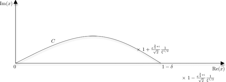
Figure 1: The deformation of the interval $[0,1-\delta]$ and the saddle points of $f(x)$.

Provided $\delta$ is sufficiently small, the interval of integration of (A.10) can be deformed into a contour asymptotically equivalent to the steepest descent path passing through

$$\bar{x}(\xi)=1+\frac{e^{\frac{3}{4}\pi i}}{\sqrt{2}}\frac{1}{\xi^{1/2}}+O\left(\xi^{-3/2}\right),\quad\xi\to\infty.$$ (A.15)

(See figure 1.) Such a deformation is not possible for the critical point

$$1-\frac{e^{\frac{3}{4}\pi i}}{\sqrt{2}}\frac{1}{\xi^{1/2}}+O\left(\xi^{-3/2}\right),\quad\xi\to\infty.$$ (A.16)

Trivial algebra gives

$$f\bigl{(}\bar{x}(\xi)\bigr{)} =i\left(\xi-\xi^{1/2}\right)-\xi^{1/2}-\frac{1}{4}+O\left(\xi^{-1/2}\right),\quad\xi\to\infty,$$ (A.17a)

$$f^{\prime\prime}\bigl{(}\bar{x}(\xi)\bigr{)} =2\sqrt{2}e^{-i\frac{\pi}{4}}\xi^{3/2}+O\left(\xi^{1/2}\right),\quad\xi\to\infty.$$ (A.17b)

The tangent to the steepest descent path at $\bar{x}$ has equation

$$x(t)=\bar{x}(\xi)+te^{-\frac{3}{8}\pi i}.$$ (A.18)

Therefore, we have

$$\begin{split}\int_{0}^{1-\delta}\exp\left(i\xi x-\frac{1}{1-x^{2}}\right)dx&=\int_{C}\exp\left(i\xi x-\frac{1}{1-x^{2}}\right)dx\\ &\sim e^{-\frac{3}{8}\pi i}\sqrt{\frac{2\pi}{\left\lvert f^{\prime\prime}\bigl{(}\bar{x}(\xi)\bigr{)}\right\rvert}}\exp\biggl{(}f\bigl{(}\bar{x}(\xi)\bigr{)}\biggr{)},\quad\xi\to\infty.\end{split}$$ (A.19)

Finally, by inserting equations (A.17) into (A.19) we arrive at (A.9), provided $\delta<\xi^{-\beta}$ and $\beta>3/4$.

∎

 

Department of Mathematics
University of Bristol
Bristol BS8 1TW, UK
Email: j.p.keating@bristol.ac.uk
Email: f.mezzadri@bristol.ac.uk
Email: b.singphu@bristol.ac.uk

16 November 2010

References

- [1] Abramowitz M. and Stegun I. Handbook of Mathematical Functions. United States Department of Commerce, National Bureau of Standards, Applied Mathematics Series 55, Washington, 1972.
- [2] Bars I. integral for the generating function in lattice gauge theory. J. Math. Phys. 21 (1980), 2678–2681.
- [3] Brouwer P. W. and Beenakker W. J. Diagrammatic method of integration over the unitary group, with applications to quantum transport mesoscopic systems. J. Math. Phys. 37 (1996), 4904–4934.
- [4] Brower R. C., Rossi P. and Tan C.-I. The external field problem for QCD. Nucl. Phys. B 190 (1981), 699–718.
- [5] Chatterjee S. and Meckes E. Multivariate normal approximation using exchangeable pairs. ALEA Lat. Am. J. Prob. Math. Stat. 4 (2008), 257–283.
- [6] Collins B. and Stolz M. Borel theorems for random matrices from the classical compact symmetric spaces. Ann. Prob. 36 (2008), 876–895.
- [7] Damgaard P. H. and Splittorff. Spectral sum rules of the Dirac operator and partially quenched chiral condensates. Nucl. Phys. B 572 (2000), 478–498.
- [8] De Wit B. and ’t Hooft G. Nonconvergence of the expansion for gauge fields on a lattice. Phys. Lett. B 69 (1977), 61–64.
- [9] Diaconis P. and Shahshahani M. On the eigenvalues of random matrices. Studies in applied probability. J. Appl. Prob. 31A (1994), 49–62.
- [10] D’Aristotile A., Diaconis P. and Newman C. Brownian motion and the classical groups. Probability, Statistics and their Applications: Papers in Honor of Rabi Bhattacharya. IMS Lect. Notes Monogr. Ser. 41 (2003), 97–116.
- [11] Diaconis P. and Evans S. N. Linear functionals of eigenvalues of random matrices. Trans. Amer. Math. Soc. 353 (2001), 2615–2633.
- [12] Feller W. An Introduction to Probability Theory and Its Applications. Vol. II, second edition. John Wiley & Sons, Inc., New York, 1970.
- [13] Haake F., Kuś M., Sommers H.-J., Schomerus H. and Życzkowski K. Secular determinants of random unitary matrices. J. Phys. A: Math. Gen. 29 (1996), 3641–3658.
- [14] Hughes C. P. and Rudnick Z. Mock-Gaussian behaviour for linear statistics of classical compact groups. Random matrix theory. J. Phys. A: Math. Gen. 36 (2003), 2919–2932.
- [15] Johansson K. On random matrices from the classical compact group. Ann. Math. (2) 145 (1997), 519–545.
- [16] Macdonald I. G. Symmetric functions and Hall polynomials. Second edition. Oxford University Press, New York, 1995.
- [17] Meckes E. An Infinitesimal Version of Stein’s Method of Exchangeable Pairs. PhD Thesis, Stanford University, 2006.
- [18] Meckes E. Linear functions on the classical matrix groups. Trans. Amer. Math. Soc. 360 (2008), 5355–5366.
- [19] Moiseyev N. Quantum theory of resonances: calculating energies, widths and cross-sections by complex scaling. Phys. Rep. 302 (1998), 212–293.
- [20] Okołowicz J., Płoszajczak M. and Rotter I. Dynamics of quantum systems embedded in a continuum. Phys. Rep. 374 (2003), 271–383.
- [21] Pastur L. and Vasilchuk V. On the moments of traces of classical groups. Commun. Math. Phys. 252 (2004), 149–166.
- [22] Samuel S. integrals, , and the De Wit-’t Hooft anomalies. J. Math. Phys. 21 (1980), 2695–2703.
- [23] Schlittgen B. and Wettig T. Generalizations of some integrals over the unitary group. J. Phys. A: Math. Gen. 36 (2003), 3195–3201.
- [24] Soshnikov A. The central limit theorem for local linear statistics in the classical compact groups and related combinatorial identities. Ann. Prob. 28 (2000), 1353–1370.
- [25] Stolz M. On the Diaconis-Shahshahani method in random matrix theory. J. Algeb. Comb. 22 (2005), 471–491.