Strong coupling expansion Monte Carlo

Abstract:

We give an overview on recently accomplished successful generalizations of ‘worm’ or loop gas simulation methods to O($N$) and CP($N-1$) sigma models and to simple fermion models. Beside the advantage of (practically) eliminated critical slowing down we also explain additional opportunities to estimate some observables with extremely improved signal to noise levels.

HU-EP-10/52

SFB/CCP-10-78

1 Introduction and conclusions

In recent years a new approach to the simulation of statistical systems on the lattice has been developed which goes under several names: world line or loop gas formalism, all-order strong coupling (or hopping parameter) simulations or ‘worm’ algorithm methods. The key idea is to first reformulate the system as the (complete) sum of its strong coupling graphs. This refers to a very simple form of the strong coupling expansion that converges as long as the volume remains finite. At large correlation length the graphs that have to be included to obtain precise results are however of forbiddingly high order for a systematic expansion. Using algorithms similar to those proposed in [1] and [2] it has become possible on the other hand to estimate the expansion of many observables by a Monte Carlo procedure that samples a representative subset of contributions. An important bonus is that this approach has been demonstrated to at least in some cases be free of critical slowing down or free of sign problems where this is not so with known methods in the conventional formulation. The problem of efficiently producing independent long distance correlated field configurations is translated into the need of efficiently passing between the relevant large strong coupling graphs. This problem seems to be sufficiently different to make progress in cases where for instance cluster algorithms in the conventional setup do not work.

The topic has been reviewed before [3] at Lattice 2008. It also seems to be closely watched by the finite-$\mu$ QCD community and typically fills a subsection in their reviews, see [4] and Sourendu Gupta’s contribution to this conference. These may be consulted in particular in connection with progress on the sign problem. In the present contribution we mainly focus on the important successful extension to non Abelian spin models of the O($N$) and CP($N-1$) type. While the method here is not confined to two dimensions, most tests are conducted there because of asymptotic freedom and the possibility to probe deeply into the continuum limit. We also cover progress on fermions which unfortunately at present is confined to two dimensions and allows for instance simulations of the Gross Neveu model. Finally we mention here that first steps have been made toward the treatment of gauge theories, see [6].

2 The idea: Ising model as an example

A good starting point to explain the strategy is the two point correlation in the Ising model

$$\langle\sigma(u)\sigma(v)\rangle=\frac{2^{-V}\sum_{\{\sigma(x)=\pm 1\}}\mathrm{e}^{\beta\sum_{l=\langle xy\rangle}\sigma(x)\sigma(y)}\sigma(u)\sigma(v)}{2^{-V}\sum_{\{\sigma(x)=\pm 1\}}\mathrm{e}^{\beta\sum_{l=\langle xy\rangle}\sigma(x)\sigma(y)}}=\frac{Z_{2}(u,v)}{Z_{0}}.$$ (1)

Here $u,v$ are sites on a hypercubic periodic lattice of $V$ sites in arbitrary dimension. In (1) we emphasize the view of a correlation as a ratio of two partition functions with and without field insertions.

In any finite volume the expansions of $Z_{0},Z_{2}$ in powers of $\beta$ are convergent for all values of $\beta$. This includes the vicinity of the critical point and all situations where Monte Carlo simulations are performed. It will turn out that in general very high orders in $\beta$ are required to realize this convergence and achieve precision. This is not possible in a systematic truncated expansion as there are unmanageably many terms or graphs. As in other physical cases it comes to rescue that not all terms are needed. A Monte Carlo procedure will instead sample a sufficiently ‘important’ subset of high order terms. Usual systematic strong coupling expansions are restricted to small correlation lengths but, on the other hand, allow to take the thermodynamic limit of quantities like $Z_{2}/Z_{0}$ term by term in the expansion. It is through this step that a finite radius of convergence emerges which in many cases (certainly in the Ising model) corresponds to a physical phase transition.

The expansion is set up by using

$$\mathrm{e}^{\beta\sigma(x)\sigma(y)}=\sum_{k=0}^{\infty}\frac{\beta^{k}}{k!}\sigma(x)^{k}\sigma(y)^{k}$$ (2)

for each neighbor pair on each link $l=\langle xy\rangle$ introducing independent integers $k(l)=0,\ldots,\infty$ on all links. For each configuration $k\equiv\{k(l)\}$ the spins may now be summed over and the partition functions are given as

$$Z_{0}=\sum_{g\in\mathcal{G}_{0}}\beta^{\sum_{l}k(l)}W[k],\hskip 10.00002ptZ_{2}(u,v)=\sum_{g\in\mathcal{G}_{2}(u,v)}\beta^{\sum_{l}k(l)}W[k].$$ (3)

In this formula the $k$-configurations are viewed as graphs of the type shown in Fig. 1. There are $k(l)$ lines on each link. The left graph is in the set $\mathcal{G}_{0}$ where the spin summation has enforced the constraint that each site must be surrounded by an even number of lines and all different such graphs make up $\mathcal{G}_{0}$.

Figure 1: A contribution in $\mathcal{G}_{0}$ (left graph) and $\mathcal{G}_{2}$ (right graph). The boundaries are identified due to torus boundary conditions

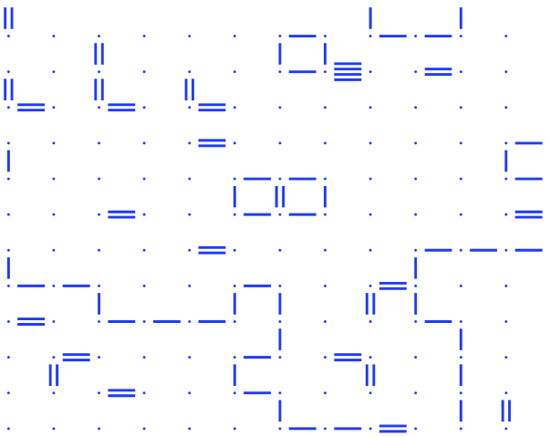
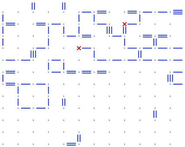
The set $\mathcal{G}_{2}(u,v)$ is visualized in the right graph in Fig. 1 with the red crosses at $u,v$ surrounded by an odd number of lines due to the extra spin insertions. The factor

$$W[k]=\prod_{l}\frac{1}{k(l)!}$$ (4)

completes the weight implied by (2).

By differentiating $\operatorname{lnZ}_{0}$ we derive the identity for a link $\langle xy\rangle=l^{\prime}$

$$\beta\langle\sigma(x)\sigma(y)\rangle=\frac{1}{Z_{0}}\sum_{g\in\mathcal{G}_{0}}\beta^{\sum_{l}k(l)}W[k]k(l^{\prime})=\langle\langle k(l^{\prime})\rangle\rangle_{0}.$$ (5)

As indicated before a typical graph is thus O($V$) in $\beta$ close to the critical point where the left hand side is O(1).

A direct simulation of the ensemble $Z_{0}$ in the form (3) was tried a long time ago in [7]. The authors designed a Monte Carlo algorithm that samples graphs in $\mathcal{G}_{0}$ (mainly) by local deformations over plaquettes. They observed critical slowing down comparable to other standard methods. Probably mainly for this reason the approach does not seem to have been pursued much further at the time. Also the accessibility of physically interesting observables was not obvious in this formulation. The two point function for example could in principle be estimated as a product over strings of $k(l)$ but this would probably be inefficient at long distance due to a large variance.

A breakthrough was achieved much later in [1] and [2]. The essential idea was a joint simulation of $Z_{0}$ and $Z_{2}$ in an ensemble with the partition function

$$\mathcal{Z}=\sum_{g\in\mathcal{G}_{2}}\beta^{\sum_{l}k(l)}W[k]=\sum_{u,v}Z_{2}(u,v)$$ (6)

where the sum over $\mathcal{G}_{2}$ without arguments is over graphs with all possible insertion points

$$\mathcal{G}_{2}=\cup_{u,v}\mathcal{G}_{2}(u,v).$$ (7)

Note that the graphs $\mathcal{G}_{0}$ contributing to $Z_{0}$ are also included as diagonal contributions with $u=v$. Expectation values are now defined as

$$\langle\langle A\rangle\rangle=\frac{1}{\mathcal{Z}}\sum_{g\in\mathcal{G}_{2}}\beta^{\sum_{l}k(l)}W[k]A[g].$$ (8)

The identity (5) now reads

$$\beta\langle\sigma(x)\sigma(y)\rangle=\frac{\langle\langle k(l)\delta_{u,v}\rangle\rangle}{\langle\langle\delta_{u,v}\rangle\rangle}=\langle\langle k(l)\rangle\rangle_{0}$$ (9)

and summing over all links $l=\langle xy\rangle$ we measure the internal energy of the original Ising model. In addition it is easy to establish the connection for general correlations

$$\langle\sigma(x)\sigma(0)\rangle=\frac{\langle\langle\delta_{x,u-v}\rangle\rangle}{\langle\langle\delta_{u,v}\rangle\rangle}$$ (10)

which in particular implies $\langle\langle\delta_{u,v}\rangle\rangle=\chi^{-1}\geqslant V^{-1}$ with the magnetic susceptibility $\chi$. The fraction of sampled graphs that belongs to $\mathcal{G}_{0}$ gets smaller toward the critical point but remains larger than one out of $V$.

In a very simple but useful generalization we include a nonnegative weight $\rho^{-1}(u-v)$,  into our strong coupling ensemble

$$\mathcal{Z}=\sum_{g\in\mathcal{G}_{2}}\beta^{\sum_{l}k(l)}W[k]\rho^{-1}(u-v)\hskip 10.00002pt\Rightarrow\hskip 10.00002pt\langle\sigma(x)\sigma(0)\rangle=\rho(x)\frac{\langle\langle\delta_{x,u-v}\rangle\rangle}{\langle\langle\delta_{u,v}\rangle\rangle}.$$ (11)

We adopt the normalization $\rho(0)=1$ and $\rho$ must respect the lattice periodicity. The advantages of this modification will be discussed in sect. 3.3.

The essential move in a Monte Carlo simulation of the $\mathcal{G}_{2}$ ensemble with partition function $\mathcal{Z}$ is now the following local update step. One may move $u$ to one of its nearest neighbors by shifting it over one of the $2D$ links attached to it. At the same time the $k(l)$ of that link is changed by $\pm 1$ (adding or removing a line of $g$). Of course similar moves may be made at $v$, alternatingly or picking randomly one of the two insertion points. These allowed moves staying within $\mathcal{G}_{2}$ may be used now as proposals for Metropolis acceptance steps. We do not describe any realization here in all details, but refer to the literature. Concrete procedures for the $\beta$ expansion discussed here may be found in [2] or [8]. Algorithms for the $\tanh\beta$ expansion of the Ising model with $k(l)\in\{0,1\}$ are discussed in detail in [9], [10].

In these papers it is numerically demonstrated that strong coupling simulations of the Ising model have very much reduced and in many cases completely eliminated critical slowing. We conclude that it is advantageous to enlarge the graph space from $\mathcal{G}_{0}$ to $\mathcal{G}_{2}$ by allowing defects. This is true even if we measure in $\mathcal{G}_{0}$ only as in (9), but we have seen that the ‘intermediate’ graphs contain even more interesting information. In these proceedings we consider the Ising discussion only as a preparation for more elaborate models and hence do not review performance results here in more detail.

3 Nonlinear sigma models

3.1 O($N$)

In [11] a generalization of the above strong coupling graph representation to the O($N$) invariant nonlinear sigma model has been given. In this case $Z_{2}$ generalizes to

$$Z_{2}(u,v)=\left[\prod_{z}\int d^{N}s\delta(s^{2}-1)\right]\mathrm{e}^{\beta\sum_{l=\langle xy\rangle}s(x)\cdot s(y)}s(u)\cdot s(v)$$ (12)

where $s(x)$ is an $N$ component unit vector integrated over the sphere. For $N=1$ the Ising model is obviously recovered. To generate an expansion in $\beta$ we again expand the Boltzmann factor on each link. To then integrate out the spins for each term in this expansion we need the integral over the sphere with an arbitrary monomial in the spin as integrand. This information follows by differentiation of the generating function with an $N$ component source $j$

$$\int d^{N}s\delta(s^{2}-1)\mathrm{e}^{j\cdot s}=\sum_{n=0}^{\infty}c[n;N](j\cdot j)^{n}$$ (13)

with coefficients

$$c[n;N]=\frac{\Gamma(N/2)}{2^{2n}n!\Gamma(N/2+n)}$$ (14)

deriving from the expansion of modified Bessel functions. Working out the combinatorics, i.e. the multiplicities of each term, we arrive at

$$\mathcal{Z}=\sum_{g\in\mathcal{G}_{2}}\beta^{\sum_{l}k(l)}W[k;N]\frac{N^{|g|}}{\mathcal{S}[g]}\times\rho^{-1}(u-v).$$ (15)

Figure 2: Schematic view of a graph $g\in\mathcal{G}_{2}$ for the O($N$) model. The divergence div $k$ means the number of lines around a site.

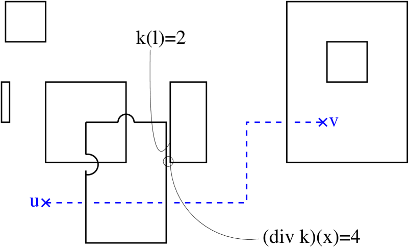
Several elements in this formula require explanation:

• The graphs $\mathcal{G}_{2}$ now differ from those in Fig. 1 only in so far that the even number of lines surrounding a site are connected pair-wise except two lines ending at $u,v$. This is visualized for a simple case in Fig. 2.

• By the pairings (corresponding to contractions of the $N$ spin components) a number of $|g|$ closed loops form in the graph $g$, each contributing a factor $N$.

• The weight $W$ collects $k(l)!$ factors and the $c[n;N]$ from the site integrations.

• The symmetry factor $\mathcal{S}[g]$ generically equals unity. Only if a graph has extra symmetries under the exchange of lines then it equals the order of this symmetry group. This is analogous to symmetry factors in Feynman diagrams. More details on this subtlety are found in the erratum of [11].

The relation between the spin correlation and the graph ensemble is changed only by the spin contraction

$$\langle s(x)\cdot s(0)\rangle=\rho(x)\frac{\langle\langle\delta_{x,u-v}\rangle\rangle}{\langle\langle\delta_{u,v}\rangle\rangle}.$$ (16)

The simulation of (15) requires in addition to the update steps outlined before reroute moves where the local line connectivity is changed. It suffices to go to $u$ (or $v$) and to randomly divorce one of the line-pairs passing through. The single line previously ending at $u$ is remarried to one of the divorcees with the other one becoming the new single line. This is again employed as a Metropolis proposal that is accepted with a well defined probability dictated by the weights in (15). By taking into account the asymmetric a priori proposal probabilities, also $\mathcal{S}[g]$ is seen to be implemented correctly.

To implement the simulation just sketched, the graph structure including its connectivity has to be mapped on a discrete structure in the Computer. This is possible by a linked list. In the language C the configuration can be coded into pointers where each line element residing on a link gets a name and points to its successor and predecessor along its closed loop. In addition there must be integer variables describing the geometrical embedding of the graph on the lattice.

The weight $N^{|g|}$ may be implemented either exactly or stochastically. In the original publication [11] the exact algorithm (R-algorithm) has been described. In this case the $N$-dependent weight (15) is fed into the Metropolis decision. Then it must be known in the reroute step, if the passing through line, that is picked for swapping the connectivity, belongs to the line connecting $u$ and $v$ or if it is part of a separate closed loop. To make this nonlocal information available requires to sometimes travel around one of the closed loops by following the corresponding pointers. As typical loop circumferences grow in the continuum limit, an elementary reroute step costs more than O(1) operations. The numerical observation in [11] can now be summarized as follows. There is (practically at least) no slowing down in units of iterations corresponding to order O($V$) elementary steps. As they cost however slightly more than O($V$) operations there is a small effective critical exponent. It was estimated around $z\approx 0.3$. This refers to the O(3) model in $D=2$ with large volume and correlation lengths $\xi=7,\ldots,65$ and to the critical $D=3$ model at $L=32,64$. The name R-algorithm derives from the fact that here $N$ may be taken also to non-integer values by continuing the weights. For integer $N$ one may formulate the I-algorithm where the weight $N^{|g|}$ is incorporated stochastically. Then each closed loop as well as the line between $u$ and $v$ carries an integer degree of freedom $i=1,2,\ldots,N$ that is independently summed over. In the reroute step, only lines with the same $i$ can join. Additional update steps are now needed to move the $i$-labels. A minimal way to do this is to randomly assign a new label to the line between $u$ and $v$ after O($V$) elementary steps. In a short test Tomasz Korzec has verified that this form of the I-algorithm shows very little critical slowing down in the O(3) model for $D=2$ and $\xi$ in the range mentioned before. A more detailed description of the R- versus I-algorithm together with numerical results is given in the paper [12] about the loop formulation of the CP($N-1$) model to which we come in sect. 3.3.

3.2 O(3) model with Nienhuis action

We now imagine to restrict the graph summation in (8) or (15) to the subclass of graphs which obey the constraint $k(l)\leqslant 1$ on all links, which can be easily implemented in the simulations. In the Ising model this changes the $\beta$ expansion into the tanh$\beta$ expansion. Thus, if we accompany the restriction by this substitution we obtain exactly the same correlation and hence $u-v$ distribution as before. In general the reduced set of graphs is equivalent to starting from

$$Z_{2}(u,v)=\left[\prod_{z}\int d^{N}s\delta(s^{2}-1)\right]\left[\prod_{l=\langle xy\rangle}\left\{1+\tilde{\beta}s(x)\cdot s(y)\right\}\right]s(u)\cdot s(v)$$ (17)

instead of (12). This is clearly a new lattice model – hence we rename $\beta\rightarrow\tilde{\beta}$ – and the question arises if it belongs to the same universality class despite its strange appearance. Such an action has been introduced before [13] and studied in detail by Nienhuis [14]. An exact solution was obtained by summing the strong coupling expansion on honeycomb lattices where the loops now cannot intersect. The critical region could be reached for $N\leqslant 2$ with $\tilde{\beta}\leqslant 1$, i.e. a nonnegative weight in (17) and universality was supported.

Figure 3: Continuum extrapolation of a step scaling function based on (17).

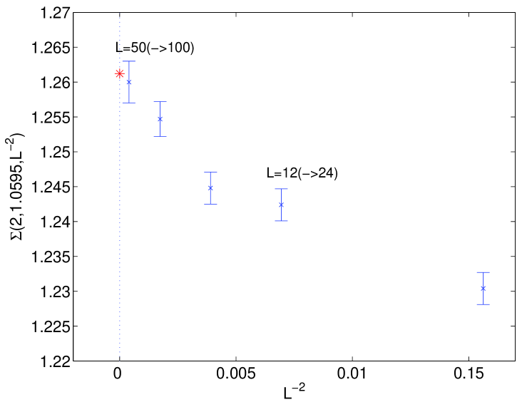
In our simulations there is absolutely no sign problem when taking $\tilde{\beta}>1$ where in the original path integral there seems to be a drastic sign problem. We thus simulated the O(3) model with $k(l)\leqslant 1$ and quickly found that no criticality was reached with $\tilde{\beta}\leqslant 1$. To investigate universality we computed a step scaling function [15] for the finite volume mass gap extracted from time slice correlations. In Fig. 3 we see that the data points accurately extrapolate to the star which is the exact universal answer known [16] for this case. These runs involve values of $\tilde{\beta}$ in the range $1.8\ldots 3.1$. Our careful conclusion is that at least for this special case a universal result is reproduced by (17) at a significant precision.

3.3 CP($N-1$)

Another class of nonlinear sigma models that are of physical interest are the $\operatorname{CP}(N-1)$ systems. There the spins label one dimensional subspaces in complex space and may be parameterized by $\phi(x)\in\mathbb{C}^{N},|\phi(x)|=1$ where $\phi$ differing by a phase have to be identified. There are two popular lattice actions compatible with this structure. One is the explicit gauge field action

$$-S[\phi,U]=\beta\sum_{x\mu}[U(x,\mu)\phi^{{\dagger}}(x)\phi(x+\hat{\mu})+U^{-1}(x,\mu)\phi^{{\dagger}}(x+\hat{\mu})\phi(x)]$$ (18)

where nearest neighbors are coupled with a U(1) gauge field $U(x,\mu)$. It is independently integrated over without an action of its own. As it can absorb local phase changes to $\phi$ the geometric structure of the model is respected. A second option is provided by the quartic action

$$-S_{q}[\phi]=2\beta_{q}\sum_{x\mu}|\phi^{{\dagger}}(x)\phi(x+\hat{\mu})|^{2}$$ (19)

which exhibits local U(1) invariance without extra fields. The standard expectation is that these actions are in the same universality class and produce the same continuum quantum field theory.

A convenient way to probe the model is by correlations of the adjoint local density  $j^{a}(x)=\phi^{{\dagger}}(x)\lambda^{a}\phi(x)$, where $\lambda_{a}$ are a basis of hermitian traceless $N\times N$ matrices normalized by $\operatorname{tr}(\lambda^{a}\lambda^{b})=2\delta^{ab}$, i.e. generalized Gell-Mann matrices. Again we focus on the two point function

$$\langle j^{a}(u)j^{a}(v)\rangle=\frac{Z_{2}(u,v)}{Z_{0}}.$$ (20)

By steps that generalize those of the Ising and O($N$) cases and which can be found in detail in [12] we construct a strong coupling representation (first for (18))

$$\mathcal{Z}=\sum_{g\in\mathcal{G}_{2}}\beta^{2\sum_{l}k(l)}W[k;N]\frac{N^{|g|}}{\mathcal{S}[g]}\times\rho^{-1}(u-v).$$ (21)

The complex field variables lead to a modified graph structure $\mathcal{G}_{2}$:

• Each line on a link carries an orientation (arrow) and they are paired at the sites in a way respecting the sense of arrows.

• There are two lines of opposite orientation running between $u$ and $v$.

• On each link there is the same number of arrows in either direction.

The last constraint is a direct consequence of integrating out the U(1) gauge field. In the exponent $k(l)$ is the number of lines per orientation. The weight $W$ is again a local product of explicitly known [12] terms and $\mathcal{S}[g]$ is the symmetry factor. The connection with the adjoint correlation can in this case be written as

$$\langle j^{a}(0)j^{b}(x)\rangle=\rho(x)\frac{2\delta_{ab}}{N(N+1)}\frac{\langle\langle\delta_{u-v,x}\rangle\rangle}{\langle\langle\delta_{u,v}\rangle\rangle}.$$ (22)

If we repeat the construction starting from the quartic action we arrive at exactly the same graph structure but obtain a different expression for $W$ and have to replace $\beta^{2}\rightarrow\beta_{q}$.

Figure 4: Autocorrelation times in the two dimensional CP(3) model in Monte Carlo time units comparable to ‘sweeps’.

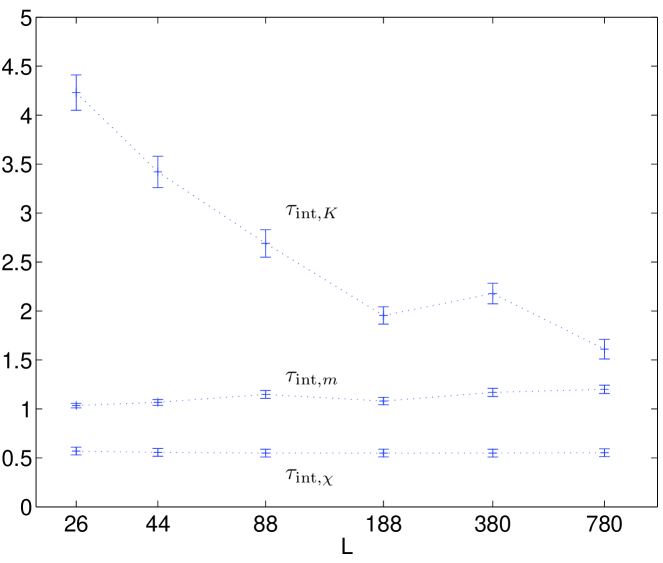
It turns out [12] that this model may be simulated by a procedure very similar to the one described for the O($N$) model. For the I-implementation treating the factor $N^{|g|}$ stochastically we show measured integrated autocorrelation times in Fig. 4. We consider a series of simulations based on (18) with $D=2,N=4$ and fixing $L/\xi\approx 10$. The observable $K$ is defined as the right hand side of (9) (summed over $l$) which also here is equivalent to the internal energy. The susceptibility $\chi$ and the mass $m$ are extracted via the correlation (22).

By computing a step scaling function the universality between the two lattice realizations of the CP($N-1$) model with actions (18) and (19) has been confirmed at high precision (see Fig. 4 in [12]) for $D=2,N=3$.

In CP($N-1$) models topology is of special interest. The status here is that the extension of (21) to include a $\theta$ term is given in [12]. A simulation of this modified system remains to be tested. Amplitudes in this case are not strictly positive any more, but it is not known for which values of $\theta$ this leads to numerically problematic sign fluctuations.

Figure 5: Effective mass as a function of time slice separation $t$ for $L=780\approx 10\xi$ in the CP(3) model.

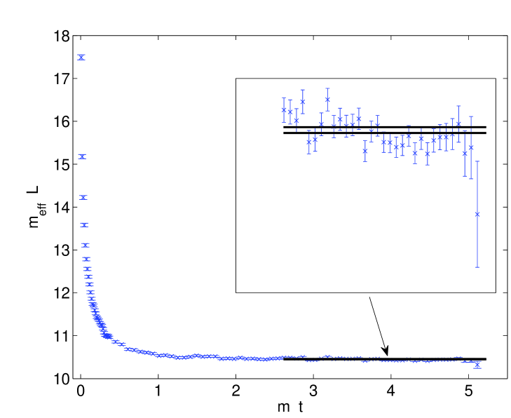
It is now time to come back to the usage of the free weight $\rho$ in our simulations. We read (22) as follows: If we are able to guess the behavior of the two point function and use this guess for $\rho(x)$, then, up to known factors, the histogram $\langle\langle\delta_{u-v,x}\rangle\rangle$ yields the correction factor that turns our guess into the exact answer. For a perfect guess, it would be constant, in other words all possible separations $u-v$ would occur with equal frequency. Up to autocorrelation effects we would then expect equal relative statistical errors at all separations. One can thus trace the exponential decay without degrading signal to noise ratio. That this really works in practice is shown in Fig. 5. Here $\rho$ was set to the scalar propagator with mass $10/L$. Similar plots are available for Ising and O($N$) simulations.

4 Fermions

In [17] the problem of a 2D Majorana-Wilson fermion in an external scalar field on a two dimensional torus was formulated as a loop gas and simulated by cluster methods. Urs Wenger first proposed [18] that in this formulation this system could alternatively be simulated with the ‘worm’ algorithm [2] which then triggered the independent study [19]. In this case the relevant partition function with two insertions is

$$\langle\xi_{\alpha}(u)\overline{\xi}_{\beta}(v)\rangle=\left[\prod_{z}\int d\xi_{1}d\xi_{2}\mathrm{e}^{-\frac{2+m}{2}\overline{\xi}\xi}\right]\left[\prod_{l=\langle xy\rangle}\mathrm{e}^{\overline{\xi}(x)P(\widehat{y-x})\xi(y)}\right]\xi_{\alpha}(u)\overline{\xi}_{\beta}(v).$$ (23)

We here integrate over two Grassmann variables per site, $P(\widehat{y-x})$ is the Wilson projector $\frac{1}{2}(1-n_{\mu}\gamma_{\mu})$ if the link is $y=x+n$ and $\overline{\xi}$ stands for $\xi^{\top}\mathcal{C}$ with charge conjugation $\mathcal{C}\gamma_{\mu}\mathcal{C}^{-1}=-\gamma_{\mu}^{\top}$. An external field is present if $m=m(x)$ is not constant. Due to the projector nature of $P$ and the Grassmann nilpotency, the expansions of the link factors have only two terms each ($k(l)=0,1$) as for the Nienhuis action. Moreover there can be at most two lines adjacent to a site and as a consequence loops and the line between $u$ and $v$ cannot intersect. A typical configuration is shown in the left panel of Fig. 6 for a massless free fermion.

Figure 6: Loop or hopping parameter expansion graph configuration for a Majorana fermion in $D=2$ (left panel) and $D=3$ (right panel).

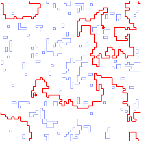
In this case the correlation is given by

$$\langle\xi_{\alpha}(x)\overline{\xi}_{\beta}(0)\rangle=\rho(x)\frac{\langle\langle\delta_{x,u-v}\Phi(k)M_{\alpha\beta}(k)\rangle\rangle}{\langle\langle\delta_{u,v}\Phi(k)\rangle\rangle}$$ (24)

where $\Phi(k)$ is a well defined and readily computable sign and $M_{\alpha\beta}(k)$ is a set of $2\times 2$ matrices which only depends on the directions in which $u$ and $v$ are approached by their connecting line. Although the observable can change sign, this two dimensional fermion has no serious sign problem, as neither the denominator nor the numerator gets very small. This is because the bulk of closed loops that close without winding around the torus are all positive. This is a specialty of two dimensional fermions which here appears as the following feature. For each closed loop there is the usual fermionic minus sign, but it is canceled by another sign. The latter arises from the trace of a string of Wilson projectors multiplied along the loops. This minus sign can be understood as the sign that arises when a spinor is parallel transported around the loop and is rotated by $2\pi$. For subtleties related to (anti)periodic boundary conditions of the finite system the reader is referred to [19] and to [20]. In this publication it is also shown how $N$ species of this loop gas can be coupled to represent and simulate the O($N$) invariant Gross Neveu model in a remarkably efficient way.

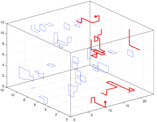
The loop representation of the Majorana fermion was generalized from $D=2$ to $D=3$ in [19]. Here we still have only two Dirac components and the efficient computability is unchanged. In the right panel of Fig. 6 we see a configuration from a simulation of a free fermion at $m=0.65$ on a $12^{2}\times 24$ lattice where we reproduced the propagator very precisely. Making however the mass smaller and/or the system much larger we very abruptly encounter the full-blown sign problem. The reason is that in $D=3$ the positivity of loops only holds as long as they are planar. If non planar loops become abundant, the spin factor assumes all values in Z(8) and does not cancel the Fermi minus any longer. Instead of Z(8) there would formally be a U(1) in the continuum, which is reduced to Z(8) on the lattice along with rotations being reduced to the hypercubic subgroup. This fermionic sign problem is presently unsolved. We consider the simple $D=3$ Majorana fermion as a good laboratory for further thinking.

5 Triviality of $\varphi^{4}$ theory

In four dimensions the number one textbook example for a quantum field theory with a self-interacting real scalar field is believed to be trivial, i.e. a free field, once the continuum limit is taken. While this is rigorously known to be the case for $D>4$ and false for $D<4$ in the borderline case of $D=4$ the belief in triviality rests on numerical demonstrations. As a byproduct of the strong coupling reformulation discussed here, we have found a very much improved handle on such numerical checks for the Ising limit of $\varphi^{4}$ which is the most interesting parameter range for triviality. One of the techniques to obtain rigorous bounds in $D>4$ has been developed by Aizenman [21]. He uses nothing but the all-order strong coupling form that we have developed in sect. 2,  called random current representation by him. Quantized currents $k(l)$ flow through the links and are conserved mod 2 at sites, with two sources at $u$ and $v$. By borrowing his replica trick and a graph theoretical proposition we could establish [8] the following identity for the Ising model at arbitrary $D$ and volume $L^{D}$

$$g_{R}=-\frac{\chi_{{}_{4}}}{\chi^{2}}(m_{R})^{D}=2z^{D}\langle\langle\mathcal{X}\rangle\rangle_{(g,g^{\prime})\in\mathcal{G}_{2}\times\mathcal{G}_{2}}.$$ (25)

In this formula for the usual renormalized coupling $g_{R}$

• $\chi$ is the 2-point susceptibility,

• $\chi_{4}$ is the 4-point (connected, symmetric phase) susceptibility,

• $m_{R}$ is a renormalized mass, for example using the second moment definition,

• any fixed values of $z=m_{R}L$ defines a renormalization scheme,

• the simulation samples two independent replica of graphs $g,g^{\prime}$ with corresponding
  $k,k^{\prime},u,u^{\prime},v,v^{\prime}$,

• $\mathcal{X}\in\{0,1\}$ is an observable computed as follows. $\mathcal{X}=1$ holds iff all four defects are in one cluster of an auxiliary bond percolation problem. The bond variables in this problem are ‘off’ only on links where $k(l)=0=k^{\prime}(l)$ holds and ‘on’ on all others. From cluster simulations we know how to efficiently compute $\mathcal{X}$.

Note that (25) implies $\chi_{{}_{4}}\leqslant 0$, i.e. the Lebowitz inequality is manifest in this estimator. The advantage of our (Aizenman’s) method lies in not having to perform a numerical cancellation to compute $\chi_{{}_{4}}$ which avoids a large significance loss. Triviality now amounts to the question whether or not $g_{R}\searrow 0$ as $L/a\rightarrow\infty$. Here for each $L/a$, $\beta$ is determined by tuning $z$ to the chosen value.

In [8] a study was made for a relatively small volume $z=2$. Although the results for $D=3,4,5$ are consistent with the triviality expectations, in $D=4$ there remained some tension in matching with the perturbative coupling evolution close to the continuum limit. Probably this must be attributed to the weakly damped fluctuations of the constant mode. We therefore made another study with $z=4$ shown in Fig. 7.

Figure 7: Cutoff dependence of the renormalized coupling for $D=4$, $z=4$. By starting integrations of the Callan Symanzik equation at the leftmost data point the lines are produced.

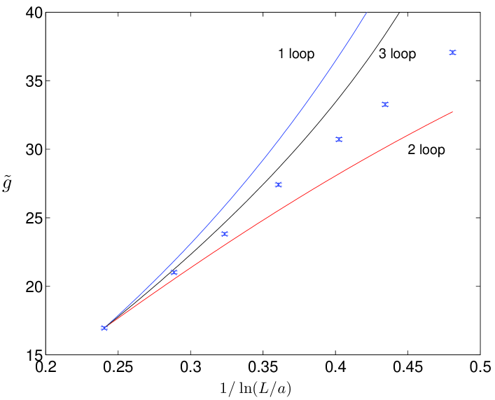
The data points with $L/a=8,\ldots,64$ have errors of only about the symbol size in spite of only modest CPU time invested on some PCs. The coupling $\tilde{g}$ may be identified with $g_{R}$ here. We see a convincing ‘convergence’ of the perturbative evolution toward the data points at small $a/L$ (left side in the plot). If we are willing to conclude that this agreement persists for yet smaller $a/L$ then triviality is established for $\varphi^{4}$ (in the Ising limit).