On Constructing the Minimal Seed of Turbulence:
Nonlinear Transient Growth

Abstract

Linear transient growth analysis is commonly used to suggest the structure of disturbances which are particularly efficient in triggering transition to turbulence in shear flows. We demonstrate that the addition of nonlinearity to the analysis can substantially change the prediction made in pipe flow from simple 2 dimensional streamwise rolls to a spanwise and cross-stream localised 3 dimensional state. This new nonlinear optimal is demonstrably more efficient in triggering turbulence than the linear optimal indicating that there are better ways to design perturbations to achieve transition.

Shear flows are ubiquitous in nature and engineering, and understanding how and why they become turbulent has huge economic implications. This has led to a number of simplified canonical problems being studied such as plane Couette flow, channel flow and pipe flow which commonly exhibit turbulent behavior even when the underlying laminar state is linearly stable. In this case, a finite amplitude perturbation is required in order to trigger turbulence and a leading question is then what is the ‘most dangerous’ or ‘smallest’ such perturbation (with the metric typically being energy). Beyond its intrinsic interest, such information is fundamentally important for devising effective control strategies to delay the onset of turbulence.

Linear transient growth analysis has commonly been used to suggest the structure of such dangerous disturbances gustav . The basic premise being that disturbances which experience the most (transient) growth are also most efficient at modifying the underlying shear to produce instability and probable transition to turbulence zikanov ; reddy . Recent improvements in our understanding of the laminar-turbulent boundary or ‘edge’, which determines whether a given initial condition leads to a turbulent episode or to the laminar state, has supported this idea albeit extended to disturbances of finite amplitude. This is because some regions of this boundary have a much smaller energy level (e.g. viswanath ) than the attracting region of the boundary-confined dynamics itano so that the minimum energy point on the edge (the most dangerous disturbance) must experience considerable energy growth as it sweeps up to the attracting plateau.

However, there are two tacit assumptions in using linear transient growth to identify critical disturbances: (1) that the energy growth experienced by the most dangerous disturbance is the largest (or near largest) possible at the critical energy; and (2) the optimal disturbance which emerges from linear transient growth analysis reasonably approximates the finite-amplitude optimal for the properly nonlinear growth calculation. Efforts to test these assumptions have concentrated on very small dimensional systems manneville or restricted the search for dangerous disturbances within small subspaces viswanath ; reddy with broadly supportive results. The only study to specifically test assumption (2) used the Blasius approximation for the boundary layer zuccher and found no qualitative difference between the nonlinear and linear optimals.

In this letter, however, we show for the first time using the full Navier-Stokes equations how nonlinearity can fundamentally change the optimal which emerges from a transient growth analysis in pipe flow at subcritical energy levels, thereby contradicting assumption (2). The significance of this new state is that: a) it provides a much more efficient way to trigger transition than the linear optimal; and b) it is 3-dimensional and shows signs of localisation thereby appearing more physically relevant than the 2-dimensional streamwise-independent linear optimal.

The transient growth problem is the optimisation question: what initial condition $\mathbf{u}(\mathbf{x},t=0)$ (added as a perturbation to the laminar flow) for the governing Navier-Stokes equations with fixed (perturbation) kinetic energy $E_{0}$ will give rise to the largest subsequent energy $E_{T}$ at a time $t=T$ later. This corresponds to maximising the functional

$$\mathscr{L} := \langle\mbox{$\frac{1}{2}$}\mathbf{u}(\mathbf{x},T)^{2}\rangle-\lambda\langle\mbox{$\frac{1}{2}$}\mathbf{u}(\mathbf{x},0)^{2}-E_{0}\rangle$$ (1)

$$-\int_{0}^{T}\langle\boldsymbol{\nu},\bigg{[}\frac{\partial\mathbf{u}}{\partial t}-16su\hat{\mathbf{z}}+2(1-4s^{2})\frac{\partial\mathbf{u}}{\partial z}$$

$$\qquad\qquad\qquad+\mathbf{u}\cdot\nabla\mathbf{u}+\nabla p-\frac{1}{Re}\nabla^{2}\mathbf{u}\bigg{]}\rangle dt$$

$$-\int_{0}^{T}\langle\Pi\nabla\cdot\mathbf{u}\rangle dt-\int_{0}^{T}\Gamma\langle\mathbf{u}\cdot\mathbf{\hat{z}}\rangle dt$$

where $\langle\,\,\rangle$ represents volume integration; $(s,\phi,z)$ are cylindrical coordinates directed along the pipe; $\lambda$, $\boldsymbol{\nu}(\mathbf{x},t)$, $\Pi(\mathbf{x},t)$ and $\Gamma(t)$ are Lagrange multipliers imposing the constraints of initial energy $E_{0}$, that the Navier-Stokes equations hold over $t\in[0,T]$, incompressibility and constant mass flux in time respectively (the system has been non-dimensionalised by the pipe diameter $D$ and the bulk velocity $U$ so that $Re:=\rho UD/\mu$ where $\rho$ is the density and $\mu$ is the dynamic viscosity, and the laminar flow is $2(1-4s^{2})\hat{\mathbf{z}}\,$). Vanishing of the variational derivatives requires that $\mathbf{u}$ must evolve according to the Navier-Stokes equations, $\boldsymbol{\nu}$ evolves according to the adjoint-Navier-Stokes equations and at times $t=0$ and $T$ we have optimality and compatibility conditions linking the two sets of variables (e.g. see guegan for details of the linearised problem). The method of solution is one of iteration as follows:

• Make an initial guess for $\mathbf{u}(\mathbf{x},t=0)$ and allow the flow to evolve according to the Navier-Stokes equations until $t=T$.

• Solve the compatibility condition for $\boldsymbol{\nu}(\mathbf{x},T)$, $\delta\mathscr{L}/\delta\mathbf{u}(\mathbf{x},T)\equiv\mathbf{u}(\mathbf{x},T)-\boldsymbol{\nu}(\mathbf{x},T)=\mathbf{0}$.

• Allow the incompressible field $\boldsymbol{\nu}(\mathbf{x},t)$ to evolve backwards in time until $t=0$ via the adjoint-Navier-Stokes equations

  $$\frac{\partial\boldsymbol{\nu}}{\partial t}+2(1-4s^{2})\frac{\partial\boldsymbol{\nu}}{\partial s}+\frac{1}{s}(\nu_{\phi}u_{s}-\nu_{s}u_{\phi})\boldsymbol{\hat{\phi}}+\mathbf{u}\cdot\nabla)\boldsymbol{\nu}$$

  $$\qquad+16s\nu_{3}\mathbf{\hat{s}}+(u_{i}\partial_{j}\nu_{i})=-\nabla\Pi-\frac{1}{Re}\nabla^{2}\boldsymbol{\nu}$$ (2)

• Move $\mathbf{u}(\mathbf{x},0)$ in the direction of the variational derivative $\delta\mathscr{L}/\delta\mathbf{u}(\mathbf{x},0)\equiv-\lambda\mathbf{u}(\mathbf{x},0)+\boldsymbol{\nu}(\mathbf{x},0)$ to increase $\mathscr{L}$ and repeat.

The algorithm should converge if $E_{0}$ does not exceed the critical energy for transition. Beyond this, sensitivity to initial conditions when $\mathbf{u}(\mathbf{x},T)$ reaches the turbulent state will lead to non-smoothness.

Both direct and adjoint equations were solved using a fully spectral, primitive variables approach. Time stepping was done using a second order fractional step scheme, checked carefully against the code of willis . The computational domain was a short periodic domain of length $\pi$ radii with typical spatial resolution of 29 real Fourier modes azimuthally, 11 real Fourier modes axially and 25 modified Chebyshev polynomials radially in each of the 8 scalar fields $(u,v,w,p,\nu_{1},\nu_{2},\nu_{3},\Pi)$. All results have been checked for robustness to resolution changes. Retention of the nonlinear terms poses a fresh technical challenge: although the adjoint equation is linear in $\boldsymbol{\nu}$, it is dependent on the evolution history of the forward variable $\mathbf{u}$ which now must be stored.

Figure 1: The evolution of the linear and nonlinear optimals at $Re=1750$. The blue (upper) line corresponds to the nonlinear optimal for $E_{0}=2\times 10^{-5}$ while the red (lower) line is the linear optimal ($E_{0}\rightarrow 0$). The nonlinear result produces more growth and actually reaches its maximum at a slightly earlier time than $T$.

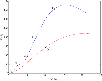
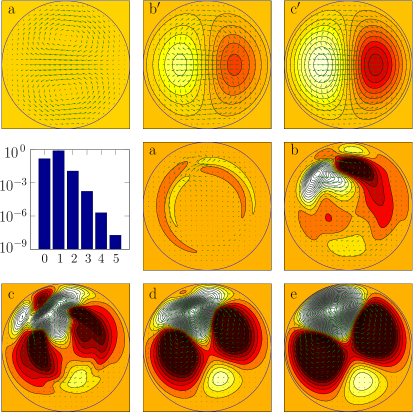
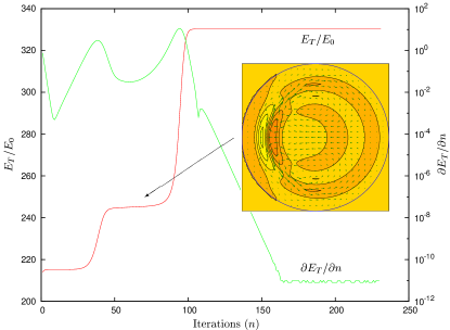
The linear transient growth optimal $\mathbf{u}_{lin}(\mathbf{x};Re)$ in pipe flow is well-known to be streamwise-independent (2D) rolls which evolve into much larger streamwise-independent streaks gustav : see figs 1 and 2. Maximum growth occurs at $T_{lin}\approx 12.2\times Re/1000\,(D/U)$ mes . Introducing nonlinearity (ie increasing $E_{0}$ from $0$), setting $T=12.2\times Re/1000\,(D/U)$ and allowing only 2D flows, leads smoothly to a modified 2D optimal $\mathbf{u}_{2D}(\mathbf{x};E_{0},Re)$ with monotonically decreasing growth consistent with previous simulations zikanov . Opening the optimisation up to fully 3D flows initially just recovers the 2D result but once $E_{0}$ crosses a small threshold $E_{3D}$ ($1.35\times 10^{-5}$ at $Re=1750$), a completely new optimal $\mathbf{u}_{3D}(\mathbf{x};E_{0},Re)$ appears. This 3D optimal emerges from the optimisation procedure after it initially appears to converge to the 2D optimal and then transiently visits an intermediate state: see fig 3. Identifying this ‘loss of stability’ of the 2D optimal provided an efficient way to compute $E_{3D}(Re)$. All optimisation results were robust over three very different choices of starting flow: a) $\mathbf{u}_{lin}$ with noise; b) the asymmetric travelling wave PK07 ; and c) a turbulent flow snapshot (all rescaled to the appropriate initial energy). This supported our supposition that the algorithm samples all possible flows of a given energy to select the global optimiser although no proof is available.

Given the intensity of the runs ($O(200)$ iterations and each iteration requires integrating forwards and backwards over the period $[0,T]$), one other Reynolds number, $Re=2250$, was selected to confirm our findings. Here, the new 3D state becomes the nonlinear optimal at $E_{3D}=4.8\times 10^{-6}$ and has essentially the same appearance as at $Re=1750$: see fig. 2. Unlike the linear optimal which is globally simple in form and undergoes an evolution that is well established (rolls advecting the mean shear to generate streaks), the 3D optimal is localised to one side of the pipe and initially has both rolls and streaks of comparable amplitude. Figures 1 and 2 show a new 2-stage evolution: a preliminary phase when the flow delocalises followed by a longer growth phase where the flow structure stabilises to essentially two 2D large-scale slow streaks sandwiching one fast streak near the boundary.

Figure 2: Three snapshots of the linear optimal (top) and five snapshots (middle & bottom) of the 3D optimal for $Re=1750$ and $E_{0}=2\times 10^{-5}$ during its evolution. Labels refer to figure 1, arrows indicate cross-sectional velocities and colours axial velocity beyond the laminar flow (white/light for positive and red/dark for negative: outside shade represents zero). The bar chart shows the ratio of energy in each streamwise Fourier mode of the initial nonlinear optimal (a).

Figure 3: $Re=1750,E_{0}=2\times 10^{-5}$. The iterations are seeded with a noisy version of the 2D optimal which converges to the 3D optimal by way of an intermediate ‘saddle’ state (shown).

Figure 4: Re=2500. The green (lowest at $t=50\,D/U$) line shows the evolution of the 3D optimal when given initial energy $\mathscr{E}_{c}$. Because it is on the laminar-turbulent boundary two nearly identical initial conditions diverge after, in this case, $220D/U$. The blue (middle at $t=50\,D/U$) line is the evolution of the 2D optimal for the exact initial energy $\mathscr{E}_{s}^{lin}$ for which the streaks become linearly unstable. The red (upper at $t=50\,D/U$) line shows the 2D optimal given initial energy $\mathscr{E}_{c}^{lin}$ and allowed to evolve until it reaches a maximum amplitude whereupon $0.1\%$ by amplitude unstable perturbation is added. Again the laminar-turbulent boundary can be identified.

For $E_{0}>2\times 10^{-5}$ at $1750$ and $6.25\times 10^{-6}$ at $2250$, the iterative procedure fails to converge. In either case, a direct numerical simulation starting with the 3D optimal at the highest energy value yielding convergence does not reveal a turbulent episode. This implies that the critical energy level, $\mathscr{E}_{c}(Re)$, for transition has not been reached . The reasons for this energy ‘gap’ are unclear and leaves open the possibility that a further new optimal may emerge. It is worth noting that the end state of the 3D nonlinear optimal decays more quickly that of the 2D optimal (which is in fact a close approximation of the least decaying eigenmode). Increasing the optimisation time, $T$, will therefore lead to the recovery of the 2D optimal at larger values of $E_{0}$. We then expect to able to converge onto the 3D optimal at correspondingly larger values of $E_{0}$, allowing the gap from $E_{3D}$ to $\mathscr{E}_{c}$ to be closed.

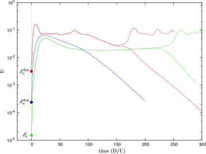
What can be tested, however, is whether the 3D optimal is more efficient at triggering turbulence than the linear optimal when rescaled. Taking the initial condition $A\mathbf{u}_{3D}(\mathbf{x};2\times 10^{-5},1750)$, we gradually increase the rescaling factor $A$ until $E_{0}=\mathscr{E}_{c}(Re)$ is reached. Calculating the corresponding quantity for the linear optimal turns out to be less clearly defined because some 3D noise is needed to trigger turbulence. As a result we make 2 different estimates, one strictly conservative and the other more realistic. The first $\mathscr{E}_{s}^{lin}$ is obtained by taking $A\mathbf{u}_{lin}(\mathbf{x};1750)$ and finding the initial energy for which the resultant streaks are just linearly unstable in this periodic domain zikanov ; reddy . In the second $\mathscr{E}_{c}^{lin}$, the same initial condition was used but $0.1\%$ of the most unstable perturbation (as found from the previous computation) is added to the streaks when they reach maximum amplitude. $\mathscr{E}_{s}^{lin}$ should be a (low) conservative estimate but even this is O(10) times larger than $\mathscr{E}_{c}$ at $Re=2500$ - see figure 4 - whereas the more realistic $\mathscr{E}_{c}^{lin}$ is O(100) times larger.

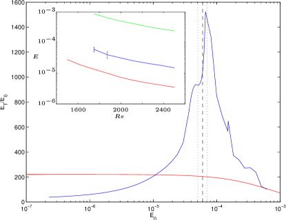
In figure 5(inset) we plot $E_{3D}$, $\mathscr{E}_{c}$ and $\mathscr{E}_{s}^{lin}$ as a function of $Re$ which emphasizes that the 2D optimal (for which the linear result is an excellent approximation) ceases to be a global maximum at an energy (at least) several orders of magnitude before it approaches the laminar-turbulent boundary. The 3D optimal, in contrast, crosses the laminar-turbulent boundary only shortly after it emerges at $E_{3D}$ (e.g. at $\approx 5\times 10^{-5}$ where $E_{3D}=1.35\times 10^{-5}$ at $Re=1750$). This means that the energy growth experienced by the 3D optimal must increase dramatically with $E_{0}$ which is illustrated in figure 5 at $Re=1750$: this growth is now a lower bound on the maximum possible for $E_{0}>2\times 10^{-5}$. Assuming that a 3D optimal will always appear at subcritical energies (reasonable as the 2D disturbance cannot trigger turbulence), the critical energy must be bounded from below by $E_{3D}$ and above by $\mathscr{E}_{c}$.

Figure 5: The effect of the initial energy on the growth of $A\mathbf{u}_{lin}$ (red) and $A\mathbf{u}_{3D}(\mathbf{x},2\times 10^{-5},1750)$ (blue) at $Re=1750$. For small $E_{0}$ the 2D result is the optimal but after $E_{3D}=1.35\times 10^{-5}$, the 3D optimal takes over. The vertical dashed line corresponds to $\mathscr{E}_{c}$, with the dotted lines being the relevant errorbars. Inset: The dependence of $E_{3D}$ (red), $\mathscr{E}_{c}$ (blue) and $\mathscr{E}_{s}^{lin}$ (green) on $Re$ ($\mathscr{E}_{c}^{lin}$ is even higher). For $Re<2000$, errorbars on $\mathscr{E}_{c}$ indicate the energy range over which short to to extended turbulent episodes are triggered.

In this letter we present the first demonstration that including nonlinearities in the problem of transient growth substantially changes the form of the optimal at energies below that needed to trigger turbulence. The significance of this result comes from the fact that transient growth analysis is currently the only constructive approach (albeit with assumptions) for identifying critical disturbances beyond exhaustive searches over initial conditions. As a result, the new 3D optimal found here supersedes the linear optimal as our current best theoretical prediction for the most dangerous disturbance in pipe flow.

There are two key directions for improving the result presented here: performing a further growth maximisation over $T$ and adopting larger, more realistic flow domains. Both represent formidable extensions even with today’s computing power. After all, the discovery of the first true nonlinear optimal has had to wait almost two decades after the linear result was established in pipe flow. In larger domains, we expect further localisation of the nonlinear optimal since energy is defined as a global quantity whereas nonlinearity is important wherever the velocity field is locally large. This strongly suggests that in a long pipe the optimal should localise fully (i.e. in the axial direction as well) which would make it an interesting focus for experiments.