Curvature Dependence of Surface Free Energy of Liquid Drops and Bubbles: A Simulation Study

Abstract

We study the excess free energy due to phase coexistence of fluids by Monte Carlo simulations using successive umbrella sampling in finite $L\times L\times L$ boxes with periodic boundary conditions. Both the vapor-liquid phase coexistence of a simple Lennard-Jones fluid and the coexistence between A-rich and B-rich phases of a symmetric binary (AB) Lennard-Jones mixture are studied, varying the density $\rho$ in the simple fluid or the relative concentration $x_{A}$ of $A$ in the binary mixture, respectively. The character of phase coexistence changes from a spherical droplet (or bubble) of the minority phase (near the coexistence curve) to a cylindrical droplet (or bubble) and finally (in the center of the miscibility gap) to a slab-like configuration of two parallel flat interfaces. Extending the analysis of M. Schrader, P. Virnau, and K. Binder [Phys. Rev. E79, 061104 (2009)], we extract the surface free energy $\gamma(R)$ of both spherical and cylindrical droplets and bubbles in the vapor-liquid case, and present evidence that for $R\rightarrow\infty$ the leading order (Tolman) correction for droplets has sign opposite to the case of bubbles, consistent with the Tolman length being independent on the sign of curvature. For the symmetric binary mixture the expected non-existence of the Tolman length is confirmed. In all cases and for a range of radii $R$ relevant for nucleation theory, $\gamma(R)$ deviates strongly from $\gamma(\infty)$ which can be accounted for by a term of order $\gamma(\infty)/\gamma(R)-1\propto R^{-2}$. Our results for the simple Lennard-Jones fluid are also compared to results from density functional theory and we find qualitative agreement in the behavior of $\gamma(R)$ as well as in the sign and magnitude of the Tolman length.

I Introduction

Curved interfaces between coexisting vapor and liquid phases (or between coexisting A-rich and B-rich phases of binary (A,B) liquid mixtures having a miscibility gap) are ubiquitous in nature. Nanoscopic spherical droplets or bubbles need to be considered in the context of nucleation phenomena 1 ; 2 ; 3 ; 4 . In nanoscopic slit pores or cylindrical pores, wetting or drying phenomena 5 ; 6 ; 7 ; 8 ; 9 typically can cause a curvature of interfaces that extend across the pore 10 ; 11 ; 12 ; 13 ; 14 . Note that phase coexistence in porous media is relevant for widespread applications 10 ; 15 ; 16 ; 17 , ranging from oil recovery out of porous rocks to devices in microfluidics.

Understanding the properties of such curved interfaces is a longstanding and difficult problem. Note that on the atomistic scale interfaces between coexisting phases are rather diffuse and the problem of understanding their structure is not fully solved. From the point of view of thermodynamics, the central quantity of interest is the interfacial tension $\gamma$ and its dependence on the radius of curvature $R$ of the droplet (or bubble). Although this problem was already mentioned by Gibbs 18 and discussed in classical papers by Tolman 19 , the subject is still controversial. Tolman introduced 19 a length $\delta(R)$, referred to as “Tolman’s length”, to describe the curvature dependence of $\gamma(R)$, but the understanding of this length is incomplete till now 20 ; 21 ; 22 ; 23 ; 24 ; 25 ; 26 ; 27 ; 28 ; 29 ; 30 ; 31 ; 32 ; Kog98 ; Nap01 ; 33 ; 34 ; 35 ; 36 ; 37 ; 38 ; 39 ; 40 .

When one considers a droplet coexisting with surrounding vapor, different definitions of the droplet radius are conceivable. One of them is the “equimolar radius” $R$, which assumes that the volumes of the two phases $V_{I}$, $V_{II}$ and their particle numbers $N_{I}$, $N_{II}$ are additive,

$$V=V_{I}+V_{II},\quad N=N_{I}+N_{II},$$ (1)

such that there is neither an excess volume nor an excess particle number associated with the interface. This definition implies that the “interfacial adsorption” is identically zero and in equilibrium both phases $I$ (liquid) and $II$ (vapor) have the same chemical potential $\mu_{I}=\mu_{II}=\mu$, since they can exchange particles. For a spherical droplet (or bubble) we have $V_{I}=4\pi R^{3}/3$, of course, and in the grand-canonical ensemble with $\mu$ and temperature $T$ as control variables, the densities of the coexisting phases $\rho_{I}(\mu,T)=N_{I}/V_{I}$, $\rho_{II}(\mu,T)=N_{II}/V_{II}$ are those of bulk liquid in equilibrium and surrounding metastable vapor. Here we disregard the conceptual problem that metastable states in the framework of statistical mechanics are not completely well-defined 3 ; 41 .

Another important concept to introduce a division between the two phases is the “surface of tension”, i.e., the surface where the surface tension acts 18 ; 19 ; 20 ; 21 . Consider, for fixed $R$ as defined above, the surface tension $\gamma(R_{p})$ 18 ; 19 ; 20 ; 21 ; 41 , i.e., the excess contribution to the thermodynamic potential, as a function of the radius $R_{p}$ where we put the dividing surface. One expects that $\gamma(R_{p})$ will exhibit a minimum for a choice of $R_{p}$ somewhere in the region of the atomistically diffuse interface, but in general there is no principle that requires that $R_{p}$ and $R$ exactly coincide. Considering the pressure difference $\Delta p$ between the coexisting phases, one can derive a generalized Laplace equation 20

$$\Delta p=2\gamma(R_{p})/R_{p}+\partial\gamma(R_{p})/\partial R_{p}.$$ (2)

Thus at the “surface of tension” where $\partial\gamma(R_{p})/\partial R_{p}=0$ the pressure difference takes its standard macroscopic form, $\Delta p=2\gamma/R_{p}$.

Now the proper definition of the Tolman length can be written as

$$\delta=\lim\limits_{R\rightarrow\infty}\delta(R)=\lim\limits_{R\rightarrow\infty}(R-R_{p}).$$ (3)

Recall that in this treatment $R_{p}$ and hence $\delta(R)$ in general can depend on $R$. Tolman 19 also suggested the approximation that $\delta$ (for a liquid droplet) is a positive constant. If this is assumed, one can show that the curvature-dependent surface tension becomes

$$\gamma(R)=\gamma(\infty)/(1+2\delta/R).$$ (4)

On the other hand, there is evidence from density functional calculations 29 ; 30 ; Kog98 ; Nap01 for liquid droplets surrounded by supersaturated vapor that actually $\delta(R)$ varies strongly with $R$, even changing its sign from a positive value at small $R$ to a small negative value at large $R$. Apart from very recent indications 39 ; 40 , most simulations, some of which are still inconclusive (see the discussion in 38 ), did not support this result. (Note that the positive values for $\delta$ in some previous simulations have not been obtained by using Eq. (4) but by a “virial route” through $1/R$–corrections to the pair correlation function of a planar interface 27 ; 38 .) There are also compelling arguments 22 ; 26 that for systems obeying a strict symmetry between the two coexisting phases, e.g., the Ising lattice gas model of a fluid that exhibits particle/hole symmetry, the Tolman length $\delta$ must be identically zero, since interchanging the identity of the coexisting phases turns a droplet into a bubble which simply means a change of sign of the radius of curvature of the interface separating them. This implies that $\gamma(R)$ for such symmetric systems can only be a function of $R^{2}$, invalidating Eq. (4) even for arbitrarily large $R$.

There appears to be consensus about the uniqueness of the $1/R$ form of the leading correction to the surface tension of bubbles and droplets (given by the Tolman length) when analyzed in different frameworks. This is not so for the next–to–leading correction and even for the leading correction to the surface tension of a cylindrical interface 26 ; Hen84 . Nevertheless, a phenomenological expansion of the surface tension of an arbitrarily curved surface in powers of its curvatures can be devised using the Helfrich form. For spherical (subscript $s$) and cylindrical interfaces (subscript $c$) the following expressions are obtained 31

$$\gamma_{s}(R) = \gamma(\infty)-2\gamma(\infty)\frac{\delta}{R}+(2k+\bar{k})\frac{1}{R^{2}}\;,$$ (5)

$$\gamma_{c}(R) = \gamma(\infty)-\gamma(\infty)\frac{\delta}{R}+\frac{k}{2}\frac{1}{R^{2}}\;.$$ (6)

Here, $k$ is the bending rigidity constant and $\bar{k}$ is the rigidity constants associated with Gaussian curvature. Such a form neglects possible nonanalytic terms in $R$, and its usefulness should be judged by comparison to actual results.

In the present work, we make an attempt to study the problem of the Tolman length and of higher order corrections, both by analyzing computer simulations of simple models for fluids and fluid mixtures, and by density functional theory. The distinctive features of our work are that we apply a recent “thermodynamic” method 39 based on exploiting Eq. (1) for various finite volumes $V=L^{3}$ with periodic boundary conditions throughout and calculate $\gamma(R)$ directly via application of successive umbrella sampling methods 42 to obtain accurate estimates for the appropriate thermodynamic potential of our model systems. In subsequent sections we use the symbols $\gamma_{AB}$ for surface tension along the $A-B$ interface in a binary mixture and $\gamma_{vl}$ for vapor-liquid interfacial tension in a single component system.

The paper is organized in the following sequence. To clarify the curvature dependence in symmetrical situations, in Sec. II we present results from the study of a symmetric binary (A,B) Lennard Jones mixture whose equilibrium properties have been extensively studied in earlier works 43 ; 44 . In Sec. III, we turn attention to the vapor-to-liquid transition of the Lennard-Jones fluid, considering both droplets and bubbles on an equal footing. Previous works, with other methods, have considered droplets almost exclusively. However, our simulation setup also allows us to consider cylindrical droplets or bubbles, stabilized by the periodic boundary conditions. Such cylindrical interfaces are not only of interest to provide further constraints on the possible value of $\delta$ as defined in Eq. (3), but are also important when one considers phase coexistence in slit pores. Sec. IV discusses the problems from the point of view of density functional theory, while Sec. V summarizes our conclusions.

II The Curvature-Dependent Surface Tension in a Symmetric Binary Lennard-Jones Mixture

We study a binary fluid of $N$ point particles (labeled by index $i$, at positions $\vec{r}_{i}$ in the cubical box of finite volume $V=L^{3}$ subject to periodic boundary conditions) interacting with pairwise potentials $u(r_{ij})$ with $r_{ij}=|\vec{r}_{i}-\vec{r}_{j}|$. Starting from a full Lennard-Jones potential

$$\phi_{LJ}(r_{ij})=4\varepsilon_{\alpha\beta}[(\sigma_{\alpha\beta}/r_{ij})^{12}-(\sigma_{\alpha\beta}/r_{ij})^{6}],\quad\alpha,\beta\in A,B,$$ (7)

we construct a truncated potential as follows 44 :

$$u(r_{ij})=\phi_{LJ}(r_{ij})-\phi_{LJ}(r_{c})-(r_{ij}-r_{c})\frac{d\phi_{LJ}}{dr_{ij}}\mid_{r_{ij}=r_{c}},\mbox{for}~{}r_{ij}\leq r_{c},$$ (8)

while $u(r_{ij}\geq r_{c})=0$. This form ensures that both the potential and the force are continuous at $r=r_{c}$ 45 . The potential parameters are chosen as

$$\sigma_{AA}=\sigma_{BB}=\sigma_{AB}=\sigma,\quad r_{c}=2.5\sigma;$$ (9)

$$\varepsilon_{AA}=\varepsilon_{BB}=2\varepsilon_{AB}=\varepsilon.$$ (10)

Choosing a reduced density $\rho^{*}=1$, where

$$\rho^{*}=\rho\sigma^{3}=N\sigma^{3}/V,$$ (11)

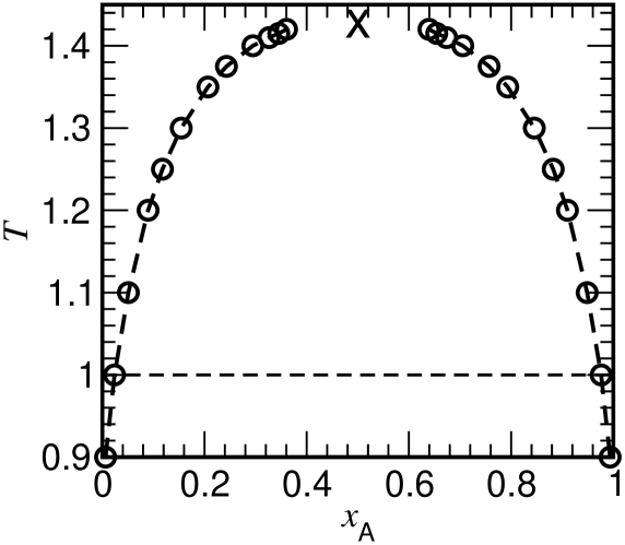
Figure 1: Phase diagram of the symmetric binary (A,B) Lennard-Jones mixture, cf. Eqs. (7)-(10), in the plane of variables $T$ and relative concentration of A particles ($x_{A}=N_{A}/N$; $N=N_{A}+N_{B}$) for fixed $N=6400$. The cross shows the critical point, as obtained previously 44 . The horizontal broken line means that phase coexistence is studied at $T=1.0$.

we work with a dense fluid and at the temperatures of interest neither the vapor-liquid transition nor crystallization is a problem. The unit of temperature $T$ is chosen such that $\varepsilon/k_{B}\equiv 1$, also throughout the paper we set the unit of length $\sigma$ to unity. The critical temperature $T_{c}$ of phase separation into an A-rich phase and a B-rich phase occurs at 44 $T=1.4230\pm 0.0005$. Using Monte Carlo methods in the semi-grandcanonical ensemble and applying a finite-size scaling analysis 46 ; 46p , the phase diagram in the plane of variables ($T,x_{A}=N_{A}/N)$ has been obtained rather accurately in the critical region 44 and we have extended it here to lower temperatures as depicted in Fig.1.

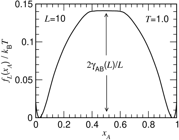
Figure 2: Effective free energy $f_{L}(x_{A},T)$ of finite-size boxes of linear dimension $L$ with $L=10$ plotted vs. $x_{A}$ at $T=1.0$, for the model of Fig. 1. The estimation of the size-dependent interfacial tension $\gamma_{AB}(L)$ is indicated.

The first task then is to obtain reliable estimates for $\gamma_{AB}=\gamma_{AB}(\infty)$, the interfacial tension between flat, infinitely extended coexisting A-rich and B-rich phases. Here we follow the standard method 47 ; 48 ; 49 ; 50 ; 51 ; 52 ; 53 ; 54 ; 55 to first sample the effective free energy $Vf_{L}(x_{A},T)=-k_{B}T\ln[P_{\Delta\mu NVT}(x_{A})/P_{\Delta\mu NVT}(x^{\rm coex}_{A})]$, presented in Fig.2, by successive umbrella sampling in the semi-grandcanonical ensemble where the chemical potential difference $\Delta\mu$ between A and B particles is independently chosen. Note that the flat region (hump) of $f_{L}(x_{A},T)$ in Fig. 2 can be interpreted as being caused by the excess free energy of two interfaces, of area $L^{2}$ each, oriented parallel to two axes of the cubic box, separating the A-rich domain from the B-rich domain, and hence

$$\gamma_{AB}(\infty)=\lim\limits_{L\rightarrow\infty}\gamma_{AB}(L),\,\,\gamma_{AB}(L)\equiv Lf_{L}(x_{A}\approx 0.5)/2.$$ (12)

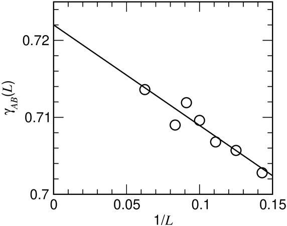
Figure 3: Extrapolation of $\gamma_{AB}(L)$ as function of $1/L$, cf. Eq. (12), in order to estimate $\gamma_{AB}(\infty)$.

Note that in finite boxes the capillary wave spectrum 5 ; 6 ; 7 ; 8 ; 20 of the interfaces is truncated, and there may be additional corrections due to the translational entropy of the interfaces, residual interactions between them, etc. Therefore, an extrapolation of $\gamma_{AB}(L)$ to $L\rightarrow\infty$ is indeed important to reach a meaningful accuracy. Such exercise is shown in Fig.3 where $\gamma_{AB}(\infty)=0.722$ is obtained from a linear extrapolation as a function of inverse linear dimension $L$ of systems.

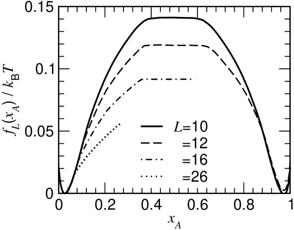
Figure 4: Effective free energy $f_{L}(x_{A},T)$ plotted vs. $x_{A}$ at $T=1.0$ for $L=10,12,16,26$, as indicated.

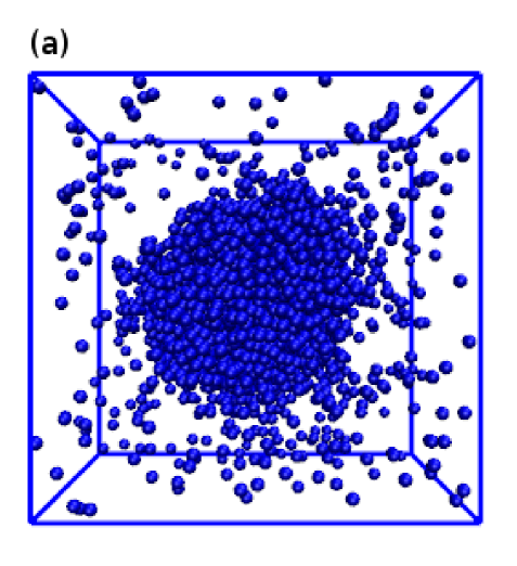
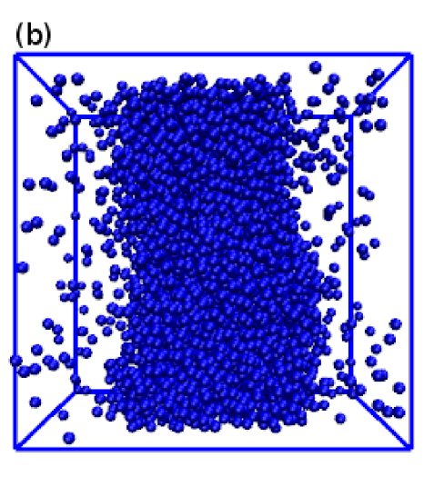
Figure 5: a) Snapshot of a spherical droplet configuration formed by A particles in the background of B-particles (not shown), for $T=1.0$, $L=24$, and $x_{A}=0.15$. b) Same as (a), but for a cylindrical droplet, choosing $x_{A}=0.27$. Note that our method does not at all suppress statistical fluctuations in the size and shape of these droplets, which therefore have spherical or cylindrical symmetry on the average only.

As described in the work of Schrader et al. 39 and Winter et al. 55 ; 56 , the curvature dependant surface tension $\gamma_{AB}(R)$ is extracted from $f_{L}(x_{A},T)$ using other parts of the same curve in Fig. 2, namely parts that reflect the coexistence of an A-rich droplet with B-rich background. Such states are found in the ascending, size-dependent part of $f_{L}(x_{A},)$, seen in Fig. 4, and correspond to spherical droplets for smaller $x_{A}$ and cylindrical droplets for larger $x_{A}$, representative snapshots of which are shown in Fig. 5. In order to be able to analyze $f_{L}(x_{A},T)$ and distinguish what fraction of this effective free energy is due to the surface free energy of the droplet and what is due to the background, a B-rich phase supersaturated in A-particles analogous to a vapor phase in the gas-liquid context, we also need to study the effective chemical potential difference $\Delta\mu_{L}(x_{A})$:

$$\frac{1}{k_{B}T}\Delta\mu_{L}(x_{A})=[\partial f_{L}(x_{A},T)/\partial x_{A}]_{T}\;,$$ (13)

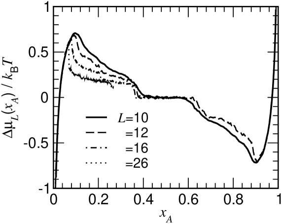
Figure 6: Plot of $\Delta\mu(X_{A})/k_{B}T$ vs. $X_{A}$ at $T=1.0$ for $L=10,12,16,26$. Data refer to a single run at each size, to illustrate the typical noise level ($200$ Monte Carlo steps per particles have been used for each window of the successive umbrella sampling). For the final analysis, $5$ such runs were averaged over.

which we present in Fig. 6. One can clearly identify the various transitions: the peak in the $\Delta\mu_{L}(x_{A})$ vs. $x_{A}$ curve for small $x_{A}$ is the transition from the homogeneous state of the box to droplet + “vapor” coexistence (the so-called droplet evaporation/condensation transition 39 ; 55 ; 56 ; 57 ; 58 ; 59 ; Tro05 ); the next step (near $x_{A}\approx 0.2)$ signifies the transition of the droplet from spherical to cylindrical shape; and finally, near $x_{A}\approx 0.35$, the transition from the cylinder to the slab configuration occurs for which we have $\Delta\mu_{L}(x_{A})=0$, of course. In order to extract information on droplet surface free energies only those parts of the $f_{L}(x_{A},T)$ vs. $x_{A}$ and $\Delta\mu_{L}(x_{A},T)$ vs. $x_{A}$ curves can be used that are not at all affected by fluctuations associated with these transitions 39 ; 55 ; 56 ; 57 ; 58 .

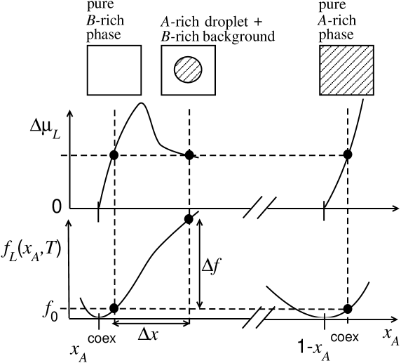
Figure 7: Schematic explanation of how the estimation of the functions $\Delta\mu_{L}(x_{A},T)$ and $f_{L}(x_{A},T)$ together allows the estimation of the concentration difference $\Delta x$ and free energy difference $\Delta f$ due to a droplet.

Fig. 7 now recalls the method by which the surface free energy $F_{s}(R)$ of the droplet and its radius $R$ are extracted 39 ; 55 ; 56 . An A-rich droplet coexists with a B-rich background having the same chemical potential as another state of pure B-rich phase. The chemical potential of the latter must be equal to those of the A-rich droplet. Use of Eq.(1) implies that one takes the bulk properties of the droplet, as a definition, equal to those of this B-rich phase, including its bulk free energy density $f_{0}$ as indicated in the lower part of the figure. The difference $\Delta f$ in Fig.7 simply is due to the surface free energy of the droplet

$$V\Delta f=4\pi R^{2}\gamma_{AB}(R).$$ (14)

On the other hand, from Eq. (1), or its analog for a binary mixture, we can readily obtain $R$ from the concentration difference $\Delta x$ between the respective states as

$$\Delta x=(1-2x_{A}^{\rm coex})(4\pi R^{3}/3L^{3}),$$ (15)

where $x^{\rm coex}_{A}$ is the concentration of the pure B-rich phase on the coexistence curve. Of course, for more precise estimation, $1-2x^{\rm coex}_{A}$ in Eq.(15) should be replaced by the difference between the compositions of the pure A-rich and B-rich phases at the considered value of $\Delta\mu$, but in practice Eq. (15) is an excellent approximation. Estimating hence $\Delta f$ and $\Delta x$ from the simulation, Eqs. (14), (15) yield the corresponding values $\gamma_{AB}(R)$ and $R$. One clearly sees that both $\Delta{\mu_{L}}(x_{A},T)$ and $f_{L}(x_{A},T)$ depend on the linear dimension $L$ of the system, which also appears explicitly in Eq. (15). However, the interpretation in terms of $\gamma_{AB}(R)$ makes only sense if this dependence on $L$ completely drops out - at least to a very good approximation.

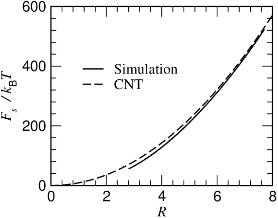
Figure 8: Plot of $F_{S}/k_{B}T$ of spherical A-rich droplet at $T=1$ for the binary symmetric LJ mixture of Fig. 1. The description in terms of the capillarity approximation of classical nucleation theory (CNT) is shown as a broken curve, using $\gamma_{AB}(\infty)=0.722$ as obtained in Fig. 3. The full curve is a superposition of independent simulation results for $L=12$, 16,18,20,22 and 24, where a running averaging was done using the combined data set.

Fig. 8 presents the resulting plot of $F_{S}(R)=4\pi R^{2}\gamma_{AB}(R)$ vs. $R$ and compares it with the capillarity approximation, $F_{S}(R)=4\pi R^{2}\gamma_{AB}(\infty)$. One sees that the latter is accurate when the resulting surface free energies are rather large, up to 600 $k_{B}T$! According to the classical nucleation theory (CNT) 1 ; 2 ; 3 ; 4 , the resulting barrier $F^{*}$ to be overcome in a homogeneous nucleation event would be $F^{*}=F_{S}(R^{*})/3$, $R^{*}$ being the radius of a critical nucleus. This implies that for $4\leq R^{*}\leq 8$ barriers $F^{*}/k_{B}T$ of about 30 to 200 result. On the other hand, one can already see from Fig. 8, however, that for very small nuclei the relative deviation from CNT increases.

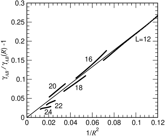
Figure 9: Plot of $\gamma_{AB}(\infty)/\gamma_{AB}(R)-1$ versus $1/R^{2}$. Here $\gamma_{AB}(\infty)$ is taken from Fig. 3, while $\gamma_{AB}(R)\equiv F_{S}(R)/4\pi R^{2}$ is estimated using Eq. (14). Ideally the estimates obtained from different values of $L$ should superimpose on a single curve. The scatter between the curves for different values of $L$ is due to residual statistical errors. The thin straight line is a fit function giving $\gamma_{AB}(\infty)/\gamma_{AB}(R)-1\simeq 2.2/R^{2}.$

We now turn to the question, whether this deviation can be accounted for in terms of Tolman’s hypothesis, Eg. (4). To test for the latter, one notes that a plot of $\gamma(\infty)/\gamma(R)$ should be equal to $1+2\delta/R$, i.e. a straight line when plotted against $1/R$. However, using the data from Fig. 8 no straight line vs. $1/R$ can be observed, while the data are compatible with a straight line when plotted against $1/R^{2}$, as seen in Fig. 9. This result agrees with the general expectation, discussed already in the introduction, that for systems that exhibit a precise symmetry between the coexisting phases the Tolman length as defined in Eq. (3) is exactly zero 22 ; 26 . Our results shown in Fig. 9, as well as a related study for the Ising model 56 , implies that instead of Eq. (4) the curvature-dependence of the surface tension $\gamma_{AB}(R)$ for symmetric mixtures can be described by

$${\gamma_{AB}(R)=\gamma_{AB}(\infty)/[1+2(\ell_{s}/R)^{2}]},$$ (16)

where the characteristic length $\ell_{s}$ at low temperatures is close to the LJ diameter $\sigma$. It remains a challenge for the future to clarify the temperature dependence of this length as $T\rightarrow T_{c}$, however. We speculate that in this limit $\ell_{s}$ simply becomes proportional to the correlation length $\xi$ of order parameter fluctuations. This is supported by explicit mean–field results for the rigidities $k$ and $\bar{k}$ Blo93 to which $\ell_{s}$ is related through $\ell_{s}^{2}=-(k+\bar{k}/2)/\gamma_{AB}(\infty)$ (see Eq. (5)) .

In Fig. 9 deliberately only the range $1/R^{2}\leq 0.12$ is shown. It should be noted that our method to construct $\gamma_{AB}(R)$ is well-defined in the limit $R\rightarrow\infty$, but as $R$ gets small, systematic errors arise: one reason is that there is a nonzero, albeit very small, probability that a state containing a droplet (or bubble), such as shown in Fig. 5a, undergoes a fluctuation to cylindrical shape (Fig. 5b) or to a homogeneous phase (Fig. 7, upper part, left most cartoon). These rare fluctuations are completely negligible for large $L$ used in Fig. 9 but should become important if linear dimensions of the order of a few $\sigma$ were used, and such linear dimensions would be needed if we were to continue the study of the behavior towards larger $1/R^{2}$. In addition, artefacts due to the periodic boundary condition are to be expected, when $L$ is only of the order of a few $\sigma$: fluctuations on the right side of the droplet would interact with fluctuations on the left side of its periodic image. Note that droplets with small $R$ require the use of small $L$, in order to ensure their stability. In this respect, our method that does not restrict statistical fluctuations beyond the use of periodic boundary conditions on the scale $L$, differs from the density functional theory (DFT) where one can consider the equilibrium of an arbitrarily small droplet (at the top $F^{*}$ of the nucleation barrier) in constrained equilibrium with surrounding metastable phase extending infinitely far away from the droplet. Due to the mean field character of DFT, this constrained equilibrium does not decay while a corresponding computer simulation clearly would result in an unstable decaying situation.

III Droplets vs. Bubbles in the Single-Component Lennard-Jones Fluid

In this section, we focus on the vapor-liquid transition of simple fluids using the LJ potential, following the work of Schrader et al. 39 . But here, in addition to spherical droplets, we also study spherical vapor bubbles as well as droplets and bubbles of cylindrical shape. While simulations of droplets surrounded by vapor are truly abundant (and such simulations have been attempted since decades 2 ), other geometries have found little attention, so far, despite their physical significance.

As in Ref. 39 we use a simple truncated LJ potential,

$$u(r_{ij}) = 4\varepsilon[(\sigma/r_{ij})^{12}-(\sigma/r_{ij})^{6}+C],\quad r\leq r_{c}=2.2^{1/6}\sigma,$$

$$u(r_{ij}) = 0,r\geq r_{c},\quad C=127/16384.$$ (17)

Thus, the potential is cut at twice the distance of the minimum, and the constant $C$ is chosen such that $u(r_{ij})$ is continuous for $r_{ij}=r_{c}$. Two temperatures $T=0.68T_{c}$ and $T=0.78T_{c}$ ($T_{c}=0.999$) were studied with the linear dimension of the simulation box varying from $L=11.3$ to $22.5$. The accuracy of the estimation of the excess free energy hump $f_{L}(\rho,T)$, $\rho$ ($=N/V$) now being the particle density, for large $L$ is enhanced by applying the Wang-Landau method 60 in addition to successive umbrella sampling. Simulation method and the data analysis 39 are rather similar to the description provided in the previous section.

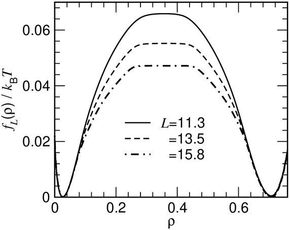
Figure 10: Effective free energy density $f_{L}(\rho)/k_{B}T$ of the single-component Lennard-Jones fluid at $T=0.78T_{c}$ plotted vs. density $\rho$ for 3 values of $L$, as indicated in the figure.

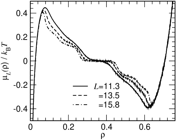
Figure 11: Plot of $\mu_{L}(\rho)/k_{B}T$ for the one-component Lennard-Jones fluid as a function of $\rho$, at $T=0.78T_{c}$, for 3 values of $L$, as indicated.

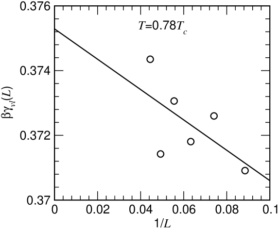
Figure 12: Extrapolation of $\beta\gamma_{vl}(L)$ as a function of $1/L$ for the simple LJ fluid at $T=0.78T_{c}$, giving $\beta\gamma_{vl}=\beta\gamma_{vl}(\infty)\simeq 0.375$. Similar exercise at $T=0.68T_{c}$ gives $\beta\gamma_{vl}\simeq 0.685$.

As an example, from the “raw data” obtained from these simulations, Figs. 10 and 11 show the free energy hump $\Delta f(\rho,T)/k_{B}T$ at the chemical potential $\mu=\mu_{\rm coex}$ yielding phase coexistence between uniform saturated vapor and liquid, as well as the derivative $\mu_{L}(\rho)/k_{B}T=(\partial(f_{L}(\rho,T)/k_{B}T)/\partial\rho)_{T}$, for $T=0.78T_{c}$. Similar to the binary LJ mixture, the flat parts of $f_{L}(\rho)$ for $\rho$ around 0.35, where $\Delta\mu_{L}(\rho)=0$, can be used to find the vapor-liquid interfacial free energies $\gamma_{vl}(\infty)$ by an extrapolation to $L\rightarrow\infty$ 47 ; 48 ; 49 ; 50 ; 51 ; 52 ; 53 , in full analogy with Eq. (12). Fig. 12 presents the counterpart of Fig. 3 in the present case, for $T=0.78T_{c}$.

The data shown in Figs. 10 and 11 are analyzed in an analogous manner as explained in the context of Fig. 7. The extension of this method to the case of bubbles is completely straightforward: one simply uses the part of the $\mu_{L}(\rho)$ and $f_{L}(\rho)$ curves near $\rho=0.6$ rather than near $\rho=0.1$ in Figs. 10, 11. While traditionally droplets have been identified as clusters of connected particles (e.g. 32 ), such methods are not at all straightforward to generalize in order to identify bubbles: the present thermodynamic method clearly has an advantage here. Also the extension to cylindrical surfaces is straightforward - we simply have to replace Eq. (14) by an expression involving the surface area $2\pi RL$ of a cylinder surface,

$$V\Delta f^{\rm cyl}=2\pi RL\gamma_{vl}^{\rm cyl}(R),$$ (18)

and Eq. (15) becomes modified by an expression containing the volume of the cylinder, $\pi R^{2}L$, rather than that of the sphere, $4\pi R^{3}/3$, so that

$$\Delta x=(\rho_{\ell}-\rho_{v})\pi R^{2}/L^{2}.$$ (19)

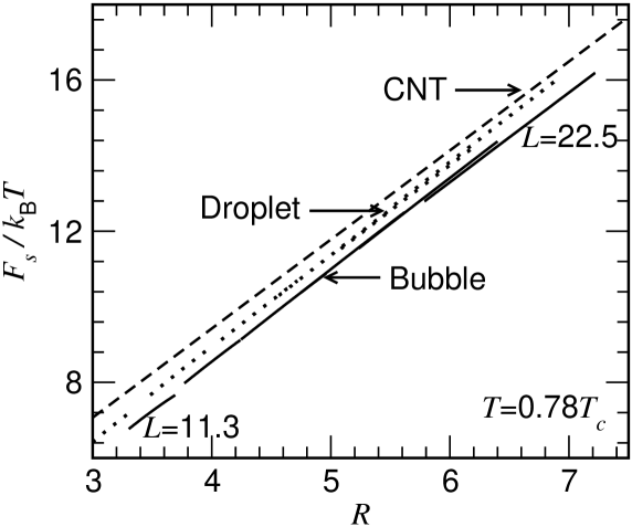
Figure 14: Same as Fig. 13, but for cylindrical droplets and bubbles. Note that, here the $y$-axis corresponds to the surface free energy per unit height of the cylinder.

Fig. 13 presents the counterpart of Fig. 8 for the single-component fluid, plotting $F_{S}/k_{B}T$ vs. the sphere radius, both for droplets and bubbles, and compares them to the capillarity approximation (CNT) where, of course, there is no difference between droplets and bubbles. Indeed, we see that CNT overestimates the correct surface free energies somewhat, and $F_{S}(R)$ for bubbles falls clearly below the result for droplets (such a difference cannot occur in symmetric models). Fig. 14 presents the results for cylindrical geometries.

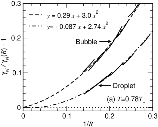
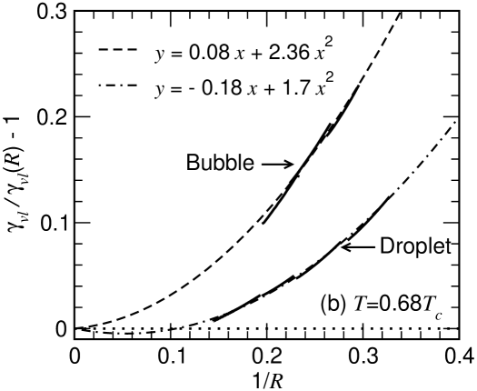
Figure 15: Plots of $\gamma_{vl}(R)/\gamma_{vl}(\infty)-1$ vs. $1/R$ for spherical droplets and bubbles for the LJ fluid at (a) $T=0.78T_{c}$ and (b) $T=0.68T_{c}$. Fits to the functional forms (III) are included.

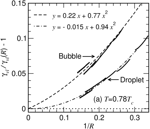
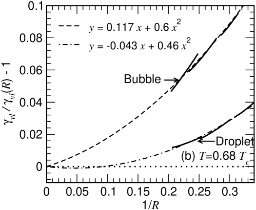
Figure 16: Same as Fig. 15, but for cylindrical droplets and bubbles.

Figs. 15 and 16 show our attempts to extract a Tolman length from the results of $\gamma_{vl}(R)$ for both droplets and bubbles with spherical as well as cylindrical shapes. Motivated by the result for symmetric systems, Eq. (16), where a quadratic term in $1/R$ is present while the linear term being absent for symmetry reasons, we now assume the presence of both linear and quadratic terms and attempt to fit data to the forms:

$$\gamma_{vl}(\infty)/\gamma_{vl}(R) = 1+2\delta/R+2(\ell_{s}/R)^{2},\;\textrm{spherical droplet},$$

$$\gamma_{vl}(\infty)/\gamma_{vl}(R) = 1-2\delta/R+2(\ell_{s}/R)^{2},\;\textrm{spherical bubble},$$

$$\gamma_{vl}(\infty)/\gamma_{vl}(R) = 1+\delta/R+2(\ell_{c}/R)^{2},\;\textrm{cylindrical droplet},$$

$$\gamma_{vl}(\infty)/\gamma_{vl}(R) = 1-\delta/R+2(\ell_{c}/R)^{2},\;\textrm{cylindrical bubble}.$$ (20)

Eqs. (III) assume that in the leading order, droplets and bubbles, where one goes from a convex to a concave interface, just differ by a change of sign. The lengths $\ell_{s}$ and $\ell_{c}$ are related to the rigidities $k$ and $\bar{k}$ introduced in Eqs. (5) and (6) by

$$\ell_{s}^{2} = 2\delta^{2}-\frac{2k+\bar{k}}{2\gamma_{vl}(\infty)}$$ (21)

$$\ell_{c}^{2} = \frac{\delta^{2}}{2}-\frac{k}{4\gamma_{vl}(\infty)}\;.$$ (22)

Upon comparing Eqs. (III) to the actual results obtained from unconstrained fits to the simulation data, quoted in Figs. 15 and 16, we observe a clear indication of linear correction, having a positive sign for bubble while being negative for droplet. This tentatively implies a negative Tolman length of order $\delta\approx-0.07\pm 0.04$ for $T=0.68T_{c}$ and $\delta\approx-0.11\pm 0.06$ for $T=0.78T_{c}$. Of course, the large error bars which we simply extract from the scatter of the four individual estimates (droplets and bubbles of spherical and cylindrical shapes) assuming that the symmetries postulated in Eqs. (III) holds, are somewhat disappointing. Of course, the possibility of systematic effects due to higher order terms $\propto$ $R^{-3},R^{-4}$ etc. cannot be ruled out. However, the success of Eq. (16) in the symmetric case for a similar range of $1/R$ (Fig. 9) strengthens our expectation that for the present case these higher order terms are still negligible. The coefficient of the term $1/R^{2}$ is of order unity, i.e., the lengths $\ell_{s}$ and $\ell_{c}$ are of the order of $\sigma$, as found in the symmetric case. From our fits we find negative bending rigidities $k$ with a magnitude of about half a $k_{B}T$ whereas the rigidity $\bar{k}$ is consistent with zero. We also note that the lengths $\delta$ and $\ell_{s},\ell_{c}$ increase in absolute magnitude, with increasing temperature. Thus, at least there is no qualitative contradiction with the prediction that actually $\delta$ should diverge as $T\rightarrow T_{c}$ 37 . However, the smallness of $\delta$ at $T=0.78T_{c}$ precludes any hope that this possible divergence might be probed by simulations.

We also note that ten Wolde and Frenkel 32 in the analysis of their simulation results for droplets (applying a rather different method than in the present paper) suggested that $\gamma_{vl}(\infty)/\gamma_{vl}(R)-1\propto 1/R^{2}$. This was motivated by theoretical results of McGraw and Laaksonen 63 , assuming hence that $\delta=0$ for a Lennard-Jones fluid. In view of our result, that $\delta$ clearly is an order of magnitude smaller than the length $\ell_{s}$ controlling the magnitude of the $R^{-2}$ term, it is understandable why ten Wolde and Frenkel missed the existence of the Tolman correction. The strong point of the present work is the proof of a clear difference between $\gamma_{vl}(R)$ for droplets and bubbles, which is inconsistent with 63 . Figs. 13,14,15,16 give very clear evidence for the existence of this difference, which according to Eq. (III) should be

$$\Delta\gamma \equiv [\gamma_{vl}(\infty)/\gamma_{vl}(R)]_{\textrm{bubbles}}-[\gamma_{vl}(\infty)/\gamma_{vl}(R)]_{\textrm{droplets}}=4\delta/R+O(R^{-3}),\;\textrm{spheres}$$

$$\Delta\gamma \equiv [\gamma_{vl}(\infty)/\gamma_{vl}(R)]_{\textrm{bubbles}}-[\gamma_{vl}(\infty)/\gamma_{vl}(R)]_{\textrm{droplets}}=2\delta/R+O(R^{-3}),\;\textrm{cylinders}$$ (23)

Our numerical data would yield, for $T=0.78T_{c}$,

$$\Delta\gamma = 0.3811(1/R)+0.266(1/R)^{2},\quad\textrm{spheres},$$

$$\Delta\gamma = 0.2386(1/R)-0.172(1/R)^{2},\quad\textrm{cylinders}.$$ (24)

The small value of the coefficient of $1/R^{2}$, compared to the individual contributions coming from droplets and bubbles, is consistent with the expected missing quadratic term in Eq. (III). The coefficient of the linear term for spheres, on the other hand, is a factor of 1.6 larger than that for cylinders and is again consistent with the expected theoretical factor 2, which is gratifying. Also, our estimates for $\delta$ certainly are compatible with the result of van Giessen and Blokhuis 38 $\delta=-0.10\pm 0.02$.

IV RESULTS FROM DENSITY FUNCTIONAL THEORY

For the one–component Lennard–Jones fluid, specified by the interaction potential in Eq. (III), we have performed density functional calculations for the metastable bubble and droplets in spherical geometry. Here, we will treat the attractive part of the potential in a mean–field fashion which is known to lack quantitative agreement with simulations for the phase diagram or the liquid–vapor surface tension. However, the density functional approach allows us to study also the limit of large droplet radii to check the validity of the asymptotic expressions (3) and (4), thus complementing our simulation results.

As usual, the free energy functional of the fluid is split into an ideal part and an excess part,

$${\cal F}[\rho] = {\cal F}^{\rm id}[\rho]+{\cal F}^{\rm ex}[\rho]$$ (25)

with the exact form of the ideal part given by

$${\cal F}^{\rm id}[\rho] = \int d^{3}r\,f^{\rm id}(\mathbf{r})=\int d^{3}r\,\rho(\mathbf{r})\left(\ln[\rho(\mathbf{r})\Lambda^{3}]-1\right)\;.$$ (26)

Here, $\Lambda$ is the de–Broglie wavelength. The excess part is split into a reference hard–sphere part and an attractive part:

$${\cal F^{\rm ex}}[\rho] = {\cal F^{\rm hs}}[\rho]+{\cal F^{\rm att}}[\rho]\;.$$ (27)

For the hard–sphere part we fix the reference hard–sphere diameter to $\sigma$, for simplicity, and employ fundamental measure functionals which are known to be very precise in various circumstances (for recent reviews see Refs. Tar08 ; Rot10 ).

$$\beta{\cal F}^{\rm hs} = \int d\mathbf{r}\,\Phi(\{\mathbf{n}[\rho(\mathbf{r})]\})\;,$$ (28)

$$\Phi(\{\mathbf{n}[\rho(\mathbf{r})]\}) = -n_{0}\,\ln(1-n_{3})+\frac{n_{1}n_{2}-\mathbf{n}_{1}\cdot\mathbf{n}_{2}}{1-n_{3}}+\varphi(n_{3})\;\frac{n_{2}^{3}-3n_{2}\,\mathbf{n}_{2}\cdot\mathbf{n}_{2}}{24\pi(1-n_{3})^{2}}\;.$$

Here, $\Phi$ is a free energy density which is a function of a set of weighted densities $\{\mathbf{n}(\mathbf{r})\}=\{n_{0},n_{1},n_{2},n_{3},\mathbf{n}_{1},\mathbf{n}_{2}\}$ with four scalar and two vector densities. These are related to the density profile $\rho(\mathbf{r})$ by $n_{\alpha}{(\mathbf{r})}=\int d\mathbf{r}^{\prime}\rho(\mathbf{r}^{\prime})\,w^{\alpha}(\mathbf{r}-\mathbf{r}^{\prime})$. The weight functions, $\{\mathbf{w}(\mathbf{r})\}=\{w^{0},w^{1},w^{2},w^{3},\mathbf{w}^{1},\mathbf{w}^{2}\}$, depend on the hard sphere radius $R=\sigma/2$ as follows:

$$w^{3}=\theta(R-|\mathbf{r}|)\;,\qquad w^{2}=\delta(R-|\mathbf{r}|)\;,\qquad w^{1}=\frac{w^{2}}{4\pi R}\;,\qquad w^{0}=\frac{w^{2}}{4\pi R^{2}}\;,$$

$$\mathbf{w}^{2}=\frac{\mathbf{r}}{|\mathbf{r}|}\delta(R-|\mathbf{r}|)\;,\qquad\mathbf{w}^{1}=\frac{\mathbf{w}^{2}}{4\pi R}\;.$$ (29)

The reference hard–sphere free energy functional in Eq. (28) is completed upon specification of the function $\varphi(n_{3})$. With the choice $\varphi=1$ we obtain the original Rosenfeld (RF) functional Ros89 , consistent with the Percus–Yevick equation of state. Upon setting

$$\varphi = 1-\frac{-2n_{3}+3n_{3}^{2}-2(1-n_{3})^{2}\ln(1-n_{3})}{3n_{3}^{2}}$$ (30)

we obtain the White Bear (WB) functional Rot02 ; Yu02 , consistent with the quasi–exact Carnahan–Starling equation of state. For the attractive part of the free energy functional we employ a mean–field (RPA) approximation motivated by the WCA potential separation WCA71 :

$${\cal F}^{\rm att}[\rho] = {\frac{1}{2}}\int d\mathbf{r}\int d\mathbf{r}^{\prime}\rho(\mathbf{r})\rho(\mathbf{r}^{\prime})\;w(|\mathbf{r}-\mathbf{r}^{\prime}|)\;,$$ (31)

$$w(|\mathbf{r}|) = \left\{\begin{matrix}u(r_{\rm min})&\qquad(r\leq r_{\rm min})\\ u(r)&\qquad(r>r_{\rm min})\end{matrix}\right.\;.$$ (32)

Here, $r_{\rm min}=2^{1/6}\sigma$ denotes the minimum location of the truncated Lennard–Jones potential $u$ defined in Eq. (III).

The phase diagram of the model can be calculated easily by evaluating the free energy functional for constant bulk densities and employing the Maxwell construction. The critical temperature, $T_{c}^{\rm mf}/\epsilon\approx 1.15$ is about 15% too large, a defect well–known in mean–field models. The discrepancies in the phase diagram between our mean–field model and simulation can be significantly reduced if the reference hard–sphere functional is used to generate a closure for the Ornstein–Zernike equation Oet05 ; Aya09 and the reference hard–sphere diameter is appropriately determined through a condition on minimal bulk free energy. However, this approach generates a lot more numerical work and the results regarding the surface tension of bubbles and droplets remain qualitatively unchanged (see below).

Planar and spherical surface tensions are obtained by extremizing the grand potential

$$\Omega[\rho] = {\cal F}[\rho]-\mu\int\rho(\mathbf{r})d\mathbf{r}$$ (33)

in the appropriate geometry, which leads to the following equation for the equilibrium density profile $\rho_{\rm eq}(\mathbf{r})$

$$\ln\frac{\rho_{\rm eq}(\mathbf{r})}{\rho_{0}}=-\beta\frac{\delta{\cal F}^{\rm ex}}{\delta\rho(\mathbf{r})}[\rho_{\rm eq}]+\beta\mu^{\rm ex}\;,$$ (34)

where the asymptotic bulk density is given by $\rho_{0}$ and $\mu\equiv\mu(\rho_{0})$ is the corresponding chemical potential ($\mu^{\rm ex}$ denotes its excess part). In planar geometry, the grand potential extremum is indeed a minimum if the boundary conditions for $\rho_{\rm eq}^{\rm planar}(z)$ are such that the coexisting vapor density $\rho_{\rm v}$ is enforced as $z\to-\infty$ and the corresponding coexisting liquid density $\rho_{\rm l}$ is enforced as $z\to\infty$. The planar surface tension thus becomes

$$\gamma_{vl} = \Omega^{\prime}[\rho_{\rm eq}^{\rm planar}(z)]-\Omega^{\prime}[\rho_{\rm v}]=\Omega^{\prime}[\rho_{\rm eq}^{\rm planar}(z)]+p(\rho_{\rm v})L\;,$$ (35)

where $\Omega^{\prime}=\Omega/A$ is the aerial grand potential density, and $L$ is the length of our numerical box in $z$–direction. In spherical geometry, the asymptotic bulk density $\rho_{0}=\lim_{r\to\infty}\rho_{\rm eq}^{\rm sph}$ has to be chosen either as an oversaturated liquid (for a vapor bubble) or an oversaturated vapor (for a liquid bubble). The corresponding extremal point of the grand potential is a saddle point which makes the extremization a bit more cumbersome. Simple iteration schemes will always diverge (“evaporating” the droplet) after some initial period of convergence. Therefore we have chosen to adopt a Picard iteration scheme along with suitable radial shifts of the whole density profile each time the Picard iteration starts to diverge. This procedure is repeated until the necessary radial shifts are below the resolution of our radial grid which is 0.001 $\sigma$. From the equilibrium profile $\rho_{\rm eq}^{\rm sph}(r)$ the equimolar droplet radius $R$ is determined by the condition of no net adsorption. For the associated surface tension it is necessary to introduce the asymptotic “inner” density of the drop $\rho_{1}\not=\rho_{0}$ which is given by the condition $\mu(\rho_{1})=\mu(\rho_{0})$. (For small drops, the actual density in the center is not necessarily equal to $\rho_{1}$.) The excess pressure within the drop is defined via our mean–field equation of state as $\Delta p=p(\rho_{1})-p(\rho_{0})$. Furthermore it is convenient to introduce the excess grand potential of the drop by

$$\Delta\Omega=\Omega[\rho_{\rm eq}^{\rm sph}(r)]+\frac{4\pi}{3}L_{\rm sph}^{3}\,p_{0}$$ (36)

where $L_{\rm sph}$ is the radius of our spherical numerical box. This excess grand potential constitutes the nucleation barrier at pressure $p_{0}$. The (equimolar) surface tension then becomes

$$\gamma_{vl}(R)=\frac{1}{4\pi R^{2}}\left(\Delta\Omega+\frac{4\pi}{3}R^{3}\,\Delta p\right)\;,$$ (37)

The radius $R_{p}$ of the “surface of tension” is defined by the Laplace condition $\Delta p=2\gamma_{vl}(R_{p})/R_{p}$. Little algebra leads to the relations:

$$R_{p} = \left(\frac{3\Delta\Omega}{2\pi\Delta p}\right)^{\frac{1}{3}}\;,$$ (38)

$$\gamma_{vl}(R_{p}) = \left(\frac{3\Delta\Omega\Delta p^{2}}{16\pi}\right)^{\frac{1}{3}}\;.$$ (39)

$T/T_{c}$	$\rho_{v}\sigma^{3}$	$\rho_{l}\sigma^{3}$	$\gamma_{vl}\sigma^{2}/\epsilon$	$\rho_{v}\sigma^{3}$	$\rho_{l}\sigma^{3}$	$\gamma_{vl}\sigma^{2}/\epsilon$
	(DFT)			(Simulation)
0.68	0.005	0.79	0.56	0.010	0.77	0.47
0.78	0.010	0.71	0.39	0.027	0.71	0.29

Table 1: Comparison between DFT and simulation results for the coexistence densities and liquid–vapor surface tension at the two investigated temperatures.

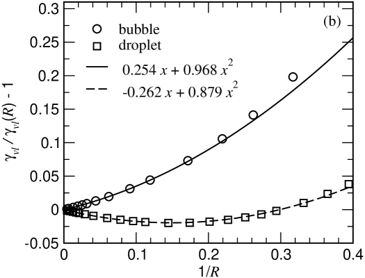
Figure 17: (a) Radius–dependent Tolman length $\delta(R)=R-R_{p}$ for bubbles and droplets with a corresponding linear fit in the range $1/R\in(0,0.1)$. (b) Surface tension ratio $\gamma_{vl}/\gamma_{vl}(R)-1$ as function of the equimolar radius $R$ for bubbles and droplets with a corresponding quadratic fit in the range $1/R\in(0,0.1)$. All results are for the temperature $T=0.78T_{c}$.

We report numerical results using the WB functional as the reference hard–sphere functional (see Eqs. (28) and (30)). Coexistence densities and planar surface tensions for the two investigated temperatures $T/T_{c}=0.68$ and 0.78 are given in Tab. 1. Since we are quite far from the critical point, the match in the coexistence densities between DFT and simulation is quite reasonable. There is, however, a mismatch in the planar surface tension of about 25%. Next we evaluated the surface tensions of bubbles and droplets for radii between 2 and approximately 200 $\sigma$. This allows us to test the asymptotic expressions for the Tolman length given in Eqs. (3) and (4). The results for $\delta(R)=R-R_{p}(R)$ and $\gamma_{vl}/\gamma_{vl}(R)-1$ are shown in Figs. 17 (for $T/T_{c}=0.78$) and 18 (for $T/T_{c}=0.68$). One can see that through a linear fit to $\delta$ as a function of $1/R$ one obtains the Tolman length to a good precision: $\delta=-0.127\pm 0.002$ for $T/T_{c}=0.78$ and $\delta=-0.122\pm 0.002$ for $T/T_{c}=0.68$. The linear terms in the quadratic fits to $\gamma_{vl}/\gamma_{vl}(R)-1$ (whose modulus should equal $2\delta$) are in agreement with these results although here the discrepancy between the bubble and droplet results are a bit larger: $\delta=-0.129\pm 0.002$ for $T/T_{c}=0.78$ and $\delta=-0.125\pm 0.008$ for $T/T_{c}=0.68$. Overall these results for the Tolman length are consistent with the simulation results of the previous section, as is the qualitative behavior of $\gamma_{vl}/\gamma_{vl}(R)-1$. The most notable discrepancy arises in the fit coefficient of the quadratic term which is about a factor 4 smaller in DFT, and thus the variation of $\gamma_{vl}(R)$ with $R$ is much less pronounced in DFT than it is in the simulation results. To understand this discrepancy partly, note that in the determination of $\gamma_{vl}(R)$ in DFT (Eq. (37) we use the mean–field bulk equation of state in the metastable domain in order to subtract the bulk grand potential of the droplet. This can be expected to lead to different results compared to the simulations where the free energy density $f_{L}(\rho,T)$ of a finite system (with box length $L$ and density $\rho$, exhibiting a stable droplet) is determined and used to subtract the bulk grand potential of the droplet. However, one can also expect that the correlations inside the droplet are not adequately captured by the mean–field treatment.

Finally we compare our DFT approach to existing DFT approaches in the literature. All DFT results have been obtained using a mean–field ansatz for the effect of attractions and differ mainly by the treatment of the hard repulsions 22 ; 28 ; 29 ; 30 ; Kog98 ; Nap01 ; 34 ; 38 . Differences in the latter manifest themselves in the absolute numbers for the surface tension whereas the results for the reduced quantity $\gamma_{vl}/\gamma_{vl}(R)$ are basically unaffected (see e.g. Refs. Kog98 ; Nap01 ). (Differences arise for smaller $R$ upon using different subtraction schemes for the bulk grand potential of the droplet). All DFT results for Lennard–Jones type liquids (with differing cut–offs, applied also at various temperatures) have so far predicted a negative Tolman length. Here we have confirmed this finding by considering also significantly larger droplets and by checking the consistency of the Tolman length extraction from both vapor bubbles and liquid droplets.

V Conclusions

In the present work a computer simulation approach to explore the surface free energy of curved interfaces is presented and applied to perform a comparative study of droplets of the minority phase in an unmixed symmetrical binary Lennard-Jones mixture and of both droplets and bubbles in the two-phase coexistence region of a simple Lennard Jones fluid. In the latter case, both droplets and bubbles of spherical and cylindrical shapes have been analyzed with the basic finding of a systematic difference between the curvature-dependent surface free energy of droplets and bubbles. Finally, also a density functional treatment of both droplets and bubbles in simple fluids is presented that supports the latter observation.

For the symmetric binary Lennard-Jones mixture, such a difference cannot occur, of course, since an interchange of A and B in the two-phase coexistence turns the minority phase into the majority phase, and a droplet becomes a bubble, or vice versa. As a consequence, Eq. (4), with a nonzero Tolmann length $\delta$, cannot apply, furthermore the dependence of the surface tension $\gamma_{AB}(R)$ on the droplet radius of curvature cannot contain any odd term in $1/R$, since $R$ changes sign when a droplet is turned into a bubble. We find that for temperatures far below criticality, the simple formula $\gamma_{AB}(R)=\gamma_{AB}(\infty)/[1+2(\ell_{s}/R)^{2}]$ {Eq. (16)} is a very good representation of our data, for radii $R$ down to about 3 Lennard-Jones diameters, and the characteristic length $\ell_{s}$ is a bit longer than a Lennard-Jones diameter (Fig. 9).

The main result for the droplets and bubbles in the simple Lennard-Jones fluid (which lacks the trivial particle-hole symmetry of the simplistic lattice gas model) is the finding that there is a significant difference between $\gamma(R)$ of droplets and bubbles (Fig. 13,14,15,16). This shows that the conventional “capillarity approximation” of the standard classical nucleation theory is not strictly valid, since the approximation does not allow for any such difference. Also theories such as those of McGraw and Laaksonen 63 , which imply that the Tolmann length $\delta$ is strictly zero and the difference $\gamma(\infty)-\gamma(R)$, to leading order, is $1/R^{2}$, are hence inconsistent with our results. We do find that this difference should be described both by a linear term $(\delta/R)$ and a quadratic term $(\ell_{s}/R)^{2}$ [Eq. (19)], while the length $\ell_{s}$ again is of the order of the Lennard-Jones diameter $\sigma$, as for the symmetric binary Lennard-Jones mixture, the Tolman length $\delta$ being an order of magnitude smaller, $\delta\approx-0.16$. This order of magnitude is compatible with the conclusion of some of the previous work 38 ; 40 . Qualitatively, these conclusions are fully confirmed by the density functional treatment (Sec. IV): note that because of the mean-field character of the latter, it does not precisely reproduce the equation of state of the model studied in the simulation and so it would be premature to ask for a quantitative “fit” of the simulation results (Fig. 15, 16) by the theory (Figs. 17, 18). However, the qualitative similarity is striking, and the order-of-magnitude agreement between the corresponding numbers is, of course, gratifying.

An important consequence of our results also is that deviations from classical nucleation theory for bubble nucleation of vapor should be distinctly larger than for droplet nucleation of liquid, at comparable radius $R$. Classical nucleation theory overestimates the nucleation barrier in the range of practical interest.

Of course, it would be interesting to study the temperature dependence of the lengths $\delta$ and $\ell_{s},\ell_{c}$, and to extend our study to other models of fluids. This will be left to future work.

Acknowledgements: This work was supported in part by the Deutsche Forschungsgemeinschaft (DFG) through the Collaborative Research Centre SFB-TR6 under grants No. TR6/A5 and TR6/N01 and through the Priority Program SPP 1296 under grants No. Bi 314/19 and Schi 853/2. S.K.D. is grateful to the Institut für Physik (Mainz) for the hospitality during his extended visits. We are also grateful to the Zentrum für Datenverarbeitung (ZDV) Mainz and the Jülich Supercomoputer Centre (JSC) for computer time. One of us (K.B.) is grateful to C. Dellago, D. Frenkel, G. Jackson and E.A. Müller for stimulating discussions.

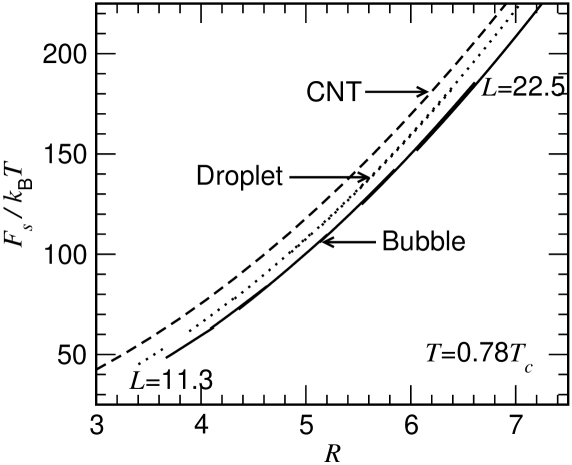
Figure 13: Plots of $F_{S}/k_{B}T$ of spherical droplets and bubbles for the one-component LJ fluid, at $T=0.78T_{c}$, as a function of sphere radius $R$. The capillarity approximation (CNT), $F_{S}/k_{B}T=4\pi R^{2}\gamma_{vl}(\infty)$ is included, using the estimate of $\gamma(\infty)$ from Fig. 12.

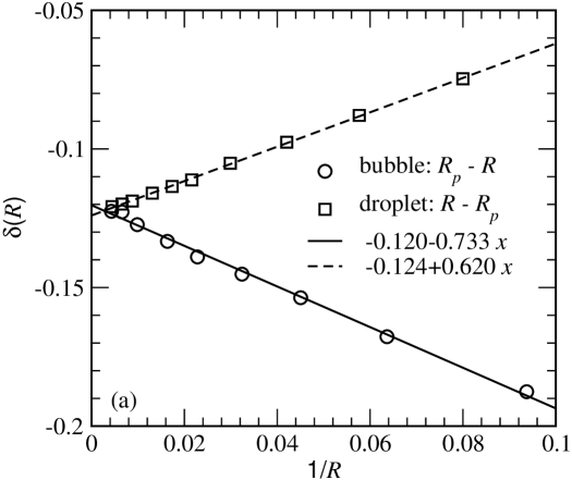
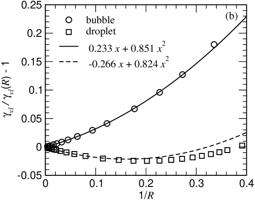
Figure 18: (a) Radius–dependent Tolman length $\delta(R)=R-R_{p}$ for bubbles and droplets with a corresponding linear fit in the range $1/R\in(0,0.1)$. (b) Surface tension ratio $\gamma_{vl}/\gamma_{vl}(R)-1$ as function of the equimolar radius $R$ for bubbles and droplets with a corresponding quadratic fit in the range $1/R\in(0,0.1)$. All results are for the temperature $T=0.68T_{c}$.

References

- (1) A.C. Zettlemoyer (ed.) Nucleation (M. Dekker, New York, 1969).
- (2) F.F. Abraham, Homogeneous Nucleation Theory (Academic, New York, 1974).
- (3) K. Binder and D. Stauffer, Adv. Phys. 25, 343 (1976); K. Binder, Rep. Progr. Phys. 50, 783 (1987).
- (4) D. Kashchiev, Nucleation: Basic Theory with Applications (Butterworth-Heinemann, Oxford, 2000).
- (5) P.G. de Gennes, Rev. Mod. Phys. 57, 825 (1985).
- (6) D.E. Sullivan and M.M. Telo da Gama, in Fluid Interfacial Phenomena (C.A. Croxton, ed.) p. 45 (Wiley, New York, 1986).
- (7) S. Dietrich, in Phase Transitions and Critical Phenomena Vol 12 (C. Domb and J.L. Lebowitz, eds.) p.1 (Academic, New York, 1988).
- (8) M. Schick, in Liquids at Interfaces (I. Charvolin, J.-F. Joanny, and J. Zinn-Justin, eds.) p. 415 (North-Holland, Amsterdam, 1990).
- (9) D. Bonn and D. Ross, Rep. Progr. Phys. 64, 1085 (2001).
- (10) L.D. Gelb, K.E. Gubbins, R. Radhakrishnan, and M. Sliwinska-Bartkowiak, Rep. Progr. Phys. 62, 1573 (1999).
- (11) A. Valencia, M. Brinkmann, and R. Lipowsky, Langmuir 17, 3390 (2001).
- (12) J. Yaneva, A. Milchev, and K. Binder, J. Chem. Phys. 121, 12632 (2004).
- (13) R. Lipowsky, M. Brinkmann, R. Dimova, T. Franke, J. Kierfeld, and X. Zhang, J. Phys.: Cond. Matter 17, S537 (2005).
- (14) K. Bucior, L. Yelash, and K. Binder, Phys. Rev. E79, 031604 (2009).
- (15) F. Schüth, K.S.W. Sing, and J. Weitkamp (eds.) Handbook of Porous Solids (Wiley-VCH, Weinheim, 2002).
- (16) A. Meller, J. Phys.: Condens. Matter 15, R581 (2003).
- (17) T.M. Squires and S.R. Quake, Rev. Mod. Phys. 77, 977 (2005).
- (18) J.W. Gibbs, The Collected Works of J. Willard Gibbs, Vol. 1, Thermodynamics (Longmans and Green, London, 1932).
- (19) R.C. Tolman, J. Chem. Phys. 16, 758 (1948); ibid 17, 118 (1949); ibid 17, 333 (1949).
- (20) J.S. Rowlinson and B. Widom, Molecular Theory of Capillarity (Clarendon, Oxford, 1982).
- (21) J.S. Henderson, in Fluid Interfacial Phenomena (C.A. Croxton, ed.) (J. Wiley & Sons, New York, 1986).
- (22) M.P.A. Fisher and M. Wortis, Phys. Rev. B29, 6252 (1984).
- (23) S.M. Thompson, K.E. Gubbins, J.P.R.B. Walton, R.A.R. Chantry and J.S. Rowlinson, J. Chem. Phys. 81, 530 (1984).
- (24) M.J.P. Nijmeijer, C. Bruin, A.B. van Woerkom, and A.F. Bakker, J. Chem. Phys. 96, 565 (1991).
- (25) E.M. Blokhuis and D. Bedeaux, Physica A184, 42 (1992); J. Chem. Phys. 97, 3576 (1992).
- (26) J.S. Rowlinson, J. Phys.: Condens. Matter 6, A1 (1994).
- (27) M.J. Haye and C. Bruin, J. Chem. Phys. 100, 556 (1994).
- (28) M. Iwanatsu, J. Phys.: Condens. Matter 6, L173 (1994).
- (29) V. Talanquer and D.W. Oxtoby, J. Phys. Chem. 99, 2865 (1995).
- (30) L. Granasy, J. Chem. Phys. 109, 9660 (1998).
- (31) A.E. van Giesen, E.M. Blokhuis, and D.J. Bukman, J. Chem. Phys. 108, 1148 (1998).
- (32) P.R. ten Walde and D. Frenkel, J. Chem. Phys. 109, 9901 (1998).
- (33) K. Koga, X. C. Zeng, and A. K. Shchekin, J. Chem. Phys. 109, 4063 (1998).
- (34) I. Napari and A. Laaksonen, J. Chem. Phys. 114, 5796 (2001).
- (35) M.P. Moody and P. Attard, Phys. Rev. Lett. 91, 056104 (2003).
- (36) J.C. Barrett, J. Chem. Phys. 124, 144705 (2006).
- (37) E.M. Blokhuis and J. Kuipers, J. Chem. Phys. 124, 074701 (2006).
- (38) J. Vrabec, G.K. Kedia, G. Fuchs, and H. Hasse, Mol. Phys. 104, 1509 (2006).
- (39) M.A. Anisimov, Phys. Rev. Lett. 98, 035702 (2007).
- (40) A.E. van Giessen and E.M. Blokhuis, J. Chem. Phys. 131, 164705 (2009).
- (41) M. Schrader, P. Virnau, and K. Binder, Phys. Rev. E79, 061104 (2009).
- (42) J.G. Sampayo, A. Malijevsky, E.A. Müller, E. de Miguel and G. Jackson, J. Chem. Phys.132, 141101 (2010).
- (43) L.D. Landau and E.M. Lifshitz, Statistical Physics (Pergamon Press, London 1958).
- (44) J. R. Henderson and J. S. Rowlinson, J. Phys. Chem. 88, 6484 (1984).
- (45) P. Virnau and M. Müller, J. Chem. Phys. 120, 10925 (2004).
- (46) S.K. Das, J. Horbach, and K. Binder, J. Chem. Phys. 119, 1547 (2003).
- (47) S.K. Das, J. Horbach, K. Binder, M.E. Fisher, and J. Sengers, J. Chem. Phys. 125, 024506 (2006); S.K. Das, M.E. Fisher, J.V. Sengers, J. Horbach and K. Binder, Phys. Rev. Lett. 97, 025702 (2006).
- (48) M.P. Allen and D.J. Tildesley, Computer Simulation of Liquids (Clarendon, Oxford, 1987).
- (49) D.P. Landau and K. Binder, A Guide to Monte Carlo Simulation in Statistical Physics, 3rd ed. (Cambridge Univ. Press, Cambridge, 2009).
- (50) M. E. Fisher, in Critical Phenomena, edited by M. S. Green (Academic, London, 1971), p. 1.
- (51) K. Binder, Phys. Rev. A25, 1699 (1982).
- (52) B.A. Berg, U. Hansmann, and T. Neuhaus, Z. Phys. B90, 229 (1993).
- (53) K. Binder, M. Müller, and W. Oed, J. Chem. Soc. Faraday Trans. 91, 2369 (1995).
- (54) J.E. Hunter and W.P. Reinhardt, J. Chem. Phys. 103, 8627 (1995).
- (55) J.J. Potoff and A.Z. Panagiotopoulos, J. Chem. Phys. 112, 6411 (2000).
- (56) J.R. Errington, Phys. Rev. E67, 012102 (2003).
- (57) P. Virnau, M. Müller, L.G. MacDowell, and K. Binder, J. Chem. Phys. 121, 2169 (2004).
- (58) R.L.C. Vink, J. Horbach, and K. Binder, Phys. Rev. E71, 011401 (2005).
- (59) M. Schrader, P. Virnau, D. Winter, T. Zykova-Timan, and K. Binder, Eur. Phys. J. ST 177, 103 (2009).
- (60) D. Winter, P. Virnau, and K. Binder, J. Phys.: Condens. Matter 21, 464118 (2009); Phys. Rev. Lett. 103, 225703 (2009).
- (61) K. Binder, Physica A319, 99 (2003).
- (62) L.G. MacDowell, P. Virnau, M. Müller, and K. Binder, J. Chem. Phys. 120, 5293 (2004).
- (63) L.G. MacDowell, V.K. Shen and J.R. Errington, J. Chem. Phys. 125, 034705 (2006).
- (64) A. Tröster, Phys. Rev. B 72, 094103 (2005).
- (65) E. M. Blokhuis and D. Bedeaux, Mol. Phys. 80, 705 (1993).
- (66) F. Wang and D.P. Landau, Phys. Rev. Lett. 86, 2050 (2001).
- (67) B.J. Block, Diploma Thesis: From Nucleation in Fluids to the Ising Model on GPU Clusters (Johannes Gutenberg-Universität Mainz, 2010, unpublished).
- (68) R. Mc Graw and A. Laaksonen, J. Chem. Phys. 106, 5284 (1997).
- (69) P.Tarazona, J. A. Cuesta, and Y. Martinez–Raton, in: A. Mulero (Ed.), Theory and Simulation of Hard-Sphere Fluids and Related Systems, Springer, Berlin (2008), pp. 247–342.
- (70) R. Roth, J. Phys.: Condens. Matter 22, 063102 (2010).
- (71) Y. Rosenfeld, Phys. Rev. Lett. 63, 980 (1989).
- (72) R. Roth, R. Evans, A. Lang, and G. Kahl, J. Phys.: Condens. Matter 14, 12063 (2002).
- (73) Y.-X. Yu and J. Wu, J. Chem. Phys. 117, 10156 (2002).
- (74) J. D. Weeks, D. Chandler, and H. C. Andersen, J. Chem. Phys. 54, 5237 (1971).
- (75) M. Oettel, J. Phys.: Condens. Matter 17, 429 (2005).
- (76) A. Ayadim, M. Oettel, and S. Amokrane, J. Phys.: Condens. Matter 21, 115103 (2009).