Local Anisotropy of Fluids using Minkowski Tensors

Abstract

Statistics of the free volume available to individual particles have previously been studied for simple and complex fluids, granular matter, amorphous solids, and structural glasses. Minkowski tensors provide a set of shape measures that are based on strong mathematical theorems and easily computed for polygonal and polyhedral bodies such as free volume cells (Voronoi cells). They characterize the local structure beyond the two-point correlation function and are suitable to define indices $0\leq\beta_{\nu}^{a,b}\leq 1$ of local anisotropy. Here, we analyze the statistics of Minkowski tensors for configurations of simple liquid models, including the ideal gas (Poisson point process), the hard disks and hard spheres ensemble, and the Lennard-Jones fluid. We show that Minkowski tensors provide a robust characterization of local anisotropy, which ranges from $\beta_{\nu}^{a,b}\approx 0.3$ for vapor phases to $\beta_{\nu}^{a,b}\rightarrow 1$ for ordered solids. We find that for fluids, local anisotropy decreases monotonously with increasing free volume and randomness of particle positions. Furthermore, the local anisotropy indices $\beta_{\nu}^{a,b}$ are sensitive to structural transitions in these simple fluids, as has been previously shown in granular systems for the transition from loose to jammed bead packs.

1 Introduction

As new experimental techniques become available, more detailed information on the nature of the fluid state can be accessed. New scattering experiments reveal the local ordering of fluids [1, 2], and confocal microscopy allows for individual particles to be tracked [3]. This richness of new data calls for new methods to characterize the morphology of equilibrium and nonequilibrium fluids and related systems.

While fluids of spherical particles usually are globally isotropic, the local environments of the particles may be anisotropic (fig. 1). Local anisotropy in jammed bead packs has recently been studied in the framework of Minkowski tensors [4]. Local anisotropy may, in fact, play a crucial role both for dynamical and equilibrium properties of particle systems. At the very least, measures of local anisotropy can be used as a local order parameter to discriminate between the various equilibrium and nonequilibrium states of an assembly of particles. This article extends the analysis given in [4] to important model fluids, namely the ideal gas (Poisson point process), the hard spheres and hard disks ensembles, and Lennard-Jones fluids. We demonstrate that the local anisotropy yields distinct evidence of the phase behavior of simple fluids; furthermore, we show that Minkowski tensors provide a robust means to its characterization.

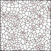
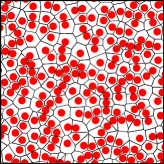
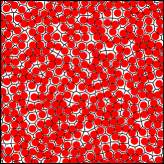
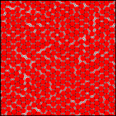
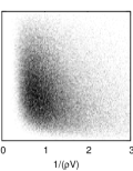
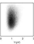
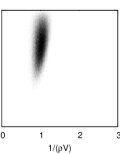
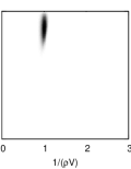
Figure 1: Histograms of local density ($x$ axis) and Voronoi cell anisotropy index ($y$ axis) in a Poisson point pattern, a dilute hard disks fluid ($\eta=32\%$), and hard disks configurations below and above the phase transition ($\eta=61\%$, $76\%$). The shape of the distribution changes characteristically with the packing density.

As a measure of local geometry in particulate matter, local anisotropy evidently competes with existing measures based on nearest-neighbor analysis, including the bond-orientational order parameters [5, 6, 7, 8], the isoperimetric ratio [9, 10] and related quantities [11], and tensorial measures such as Edwards’ configurational tensor [12], quadrons [13], and fabric / texture tensors [14]. These measures are, while undoubtedly widely and successfully applied, reliant on identifying suitable neighborhoods. Neighborhoods, by their very nature, change discontinuously, in contrast to the shape measures of Voronoi cells used in the present study. The volume distributions of Voronoi cells have been studied [15, 16, 17] and the shape of Voronoi cells is their next important property. Scalar measures of shape such as the isoperimetric ratio contain some signature of anisotropy; however, they do not discern between the generally distinct but often correlated concepts of asphericity (meaning deviation form a spherical shape) and anisotropy (meaning elongation or directedness). It is our hypothesis that explicit anisotropy measures such as the Minkowski tensors will turn out similarly useful for the identification of phase transitions in fluids and other particulate systems, while being more generic and robust in their definition than measures based on neighborhoods. Explicit anisotropy measures may also be more easily generalized to aspherical particles, relevant to liquid crystalline phases [18, 19, 20].

The article is organized as follows: In section 2.1, we restate briefly the definition of the Minkowski tensors. Section 2.2 discusses how Minkowski tensors may be used to characterize anisotropy. In section 2.3, we use Minkowski tensors of Voronoi tessellations to characterize the local anisotropy in a point pattern, such as the configuration of particles in a fluid. Sections 3 and 4 gives the results of the anisotropy analysis for an ideal gas, described by the Poisson point process, and equilibrium systems of hard spheres and disks. Section 5 applies the same analysis to point particles interacting with a Lennard-Jones potential. Section 6 shows that Minkowski tensors are both robust and sensitive measures of local geometry by applying them to the Einstein solid model.

2 Anisotropy Characterization by Minkowski Tensors

2.1 Minkowski Tensors

The description of shape requires the choice of adequate quantities that may be associated with the shape in question. Minkowski functionals, also known as Quermaßintegrale or intrinsic volumes, are scalar measures of shape defined in convex and integral geometry, based on support measures [21, 22]. Equivalently, they may be introduced as curvature-weighted integrals, as in this section.

Given a compact subset of $D$-dimensional Euclidean space $K\subset\mathbb{R}^{D}$, called a body, with a sufficiently smooth boundary, the Minkowski functionals in two and three dimensions are defined as

$$W_{0}(K) := \int_{K}{\rm d}^{D}r$$ (1)

$$W_{\nu}(K) := {\frac{1}{D}}\int_{\partial K}{\rm d}^{D-1}r\;G_{\nu}(\vec{r}),\quad 1\leq\nu\leq D,$$ (2)

where $G_{\nu}(\vec{r})$ is a symmetric combination of the principal curvatures $\kappa_{i}$ of the boundary $\partial K$. In two dimensions, $G_{1}=1,G_{2}=\kappa$, (there is only one curvature) and in three dimensions $G_{1}=1,G_{2}=\frac{1}{2}(\kappa_{1}+\kappa_{2}),G_{3}=\kappa_{1}\kappa_{2}$. The Minkowski functionals are, up to conventional prefactors, the area, the circumference, and the Euler number (in 2D) and the volume, the surface area, the integral mean curvature, and the Euler number (in 3D) of the body $K$. The set of Minkowski functionals has a number of properties which make them useful for shape analysis of physical systems [23]. In particular, by Hadwiger’s characterization theorem [21], the set of Minkowski functionals spans the space of additive, conditionally continuous and motion invariant functionals of $K$. For such functionals, the Minkowski functionals contain all the relevant morphological information about the shape of $K$.

A natural generalization of Minkowski functionals are Minkowski tensors, which arise by including tensor products of the position vector $\vec{r}$ and the outer boundary normal $\vec{n}$ in the integrals in eq. (2). In analogy to the scalar case, the Minkowski tensors span the space of additive, conditionally continuous and motion-covariant functionals [24]. Knowledge of all the Minkowski tensors provides a more complete morphological description of the body $K$ than the scalar properties alone, and allows for tensor-valued functionals of $K$ to be computed. The set of Minkowski tensors contains, analogous to the scalar case, complete morphological information about the shape of $K$. A basis of the space of tensor-valued functionals of rank two is given in table 1. In addition to the scalar Minkowski functionals, four Minkowski tensors (six in 3D) are required to span the space.

	Tensor	Matrix element $i,j$
$D=2$	$E\cdot W_{0}$	$\delta_{ij}\cdot\int_{K}{\rm d^{2}}r$
	$E\cdot W_{1}$	$\frac{1}{2}\delta_{ij}\cdot\int_{\partial K}{\rm d}r$
	$E\cdot W_{2}$	$\frac{1}{2}\delta_{ij}\cdot\int_{\partial K}{\rm d}r\;\kappa$
	$W_{0}^{2,0}$	$\int_{K}{\rm d^{2}}r\;r_{i}r_{j}$
	$W_{1}^{2,0}$	$\frac{1}{2}\int_{\partial K}{\rm d}r\;r_{i}r_{j}$
	$W_{2}^{2,0}$	$\frac{1}{2}\int_{\partial K}{\rm d}r\;\kappa\;r_{i}r_{j}$
	$W_{1}^{0,2}$	$\frac{1}{2}\int_{\partial K}{\rm d}r\;n_{i}n_{j}$

	Tensor	Matrix element $i,j$
$D=3$	$E\cdot W_{0}$	$\delta_{ij}\cdot\int_{K}{\rm d^{3}}r$
	$E\cdot W_{1}$	$\frac{1}{3}\delta_{ij}\cdot\int_{\partial K}{\rm d^{2}}r$
	$E\cdot W_{2}$	$\frac{1}{6}\delta_{ij}\cdot\int_{\partial K}{\rm d^{2}}r\;\bigl{(}\kappa_{1}+\kappa_{2}\bigr{)}$
	$E\cdot W_{3}$	$\frac{1}{3}\delta_{ij}\cdot\int_{\partial K}{\rm d^{2}}r\;\kappa_{1}\kappa_{2}$
	$W_{0}^{2,0}$	$\int_{K}{\rm d^{3}}r\;r_{i}r_{j}$
	$W_{1}^{2,0}$	$\frac{1}{3}\int_{\partial K}{\rm d^{2}}r\;r_{i}r_{j}$
	$W_{2}^{2,0}$	$\frac{1}{6}\int_{\partial K}{\rm d^{2}}r\;\bigl{(}\kappa_{1}+\kappa_{2}\bigr{)}\;r_{i}r_{j}$
	$W_{3}^{2,0}$	$\frac{1}{3}\int_{\partial K}{\rm d^{2}}r\;\kappa_{1}\kappa_{2}\;r_{i}r_{j}$
	$W_{1}^{0,2}$	$\frac{1}{3}\int_{\partial K}{\rm d^{2}}r\;n_{i}n_{j}$
	$W_{2}^{0,2}$	$\frac{1}{6}\int_{\partial K}{\rm d^{2}}r\;\bigl{(}\kappa_{1}+\kappa_{2}\bigr{)}\;n_{i}n_{j}$

Table 1: A basis for the space of rank-two additive, conditionally continuous, motion-covariant functionals in terms of Minkowski functionals $W_{\nu}$ and Minkowski tensors $W_{\nu}^{a,b}$. $E$ is the unit matrix, $\kappa=\kappa(\vec{r})$ the local curvature of the boundary contour $\partial K$ at point $\vec{r}$, $\kappa_{1}(\vec{r})$ and $\kappa_{2}(\vec{r})$ the principal curvatures of the boundary surface $\partial K$, $\vec{n}(\vec{r})$ the outer boundary normal at point $\vec{r}$.

For the mathematical details we refer the reader elsewhere [25, 26, 27], and instead only give a single example, namely the Minkowski tensor $W_{1}^{0,2}$ of a planar body $K$ which is given by

$$W_{1}^{0,2}(K)={\textstyle\frac{1}{2}}\int_{\partial K}{\rm d}r\left(\begin{array}[]{ccc}n_{1}n_{1}&n_{1}n_{2}\\ n_{2}n_{1}&n_{2}n_{2}\end{array}\right)$$ (3)

where $n_{i}$ are the components of the outer normal vector at the boundary $\partial K$ of $K$, and ${\rm d}r$ is the infinitesimal line element on the boundary $\partial K$. $W_{1}^{0,2}(K)$ can now be written in terms of three independent scalar boundary integrals

$$W_{1}^{0,2}(K)=\left(\begin{array}[]{ccc}I_{11}(K)&I_{12}(K)\\ I_{12}(K)&I_{22}(K)\end{array}\right).$$ (4)

Importantly for applications, the Minkowski tensors of a triangulated body (in the planar case, a polygon) can be written as a simple sum over all facets and thus calculated in $\mathcal{O}(N)$ time. For a polygon, the $I_{ij}(K)$ in eq. (4) are given by the three sums

$$I_{ij}(K)={\textstyle\frac{1}{2}}\sum_{f}L^{(f)}n^{(f)}_{i}n^{(f)}_{j}$$ (5)

where the index $f$ labels the edges of the polygon, and $L^{(f)}$, $\vec{n}^{(f)}$ are their lengths and outer normals respectively. An analogous formula holds in three dimensions, replacing edge lengths by facet areas. Explicit formulae for the fast and simple computation of the complete set of Minkowski tensors ($W_{0}^{2,0}$, $W_{1}^{2,0}$, $W_{2}^{2,0}$, $W_{1}^{0,2}$ in 2D and $W_{0}^{2,0}$, $W_{1}^{2,0}$, $W_{2}^{2,0}$, $W_{3}^{2,0}$, $W_{1}^{0,2}$, $W_{2}^{0,2}$ in 3D) can be found in refs. [25, 26].

Similar to the tensor of inertia, some of the Minkowski tensors, $W_{\nu}^{2,0}$, do not depend only on the shape of $K$ but also on its location. A suitable origin has to be chosen for computation of the Minkowski tensors for a given body. The tensors including only normal vectors, $W_{\nu}^{0,2}$, are translation invariant.

2.2 Anisotropy Characterization of Shapes

Having assigned a number of tensorial shape descriptors to each body $K$, we can now define an anisotropy index for each body $K$ and each Minkowski tensor $W_{\nu}^{a,b}(K)$ by the dimensionless ratio

$$\beta_{\nu}^{a,b}(K):=\frac{{\lambda}_{\rm min}(W_{\nu}^{a,b}(K))}{{\lambda}_{\rm max}(W_{\nu}^{a,b}(K))},$$ (6)

where ${\lambda}_{\rm min}(W)$, ${\lambda}_{\rm max}(W)$ are the smallest and largest eigenvalues of the $D\times D$ matrix $W$; $D$ the spatial dimension. An anisotropy index of $\beta=1$ indicates an isotropic body, and values ranging from 1 to 0 correspond to increasing degrees of anisotropy. The dimensionless anisotropy index is a pure shape measure; it is invariant under isotropic scaling of $K$, i. e. $\beta_{\nu}^{a,b}(sK)=\beta_{\nu}^{a,b}(K)$, for all $s>0$.

Note that, in the framework of this analysis, we consider any body isotropic that has Minkowski tensors proportional to the unit matrix. Bodies with $n$-fold rotation symmetries through the origin ($n\geq 3$) have degenerate eigenvalues due to the additivity of the Minkowski tensors; as a consequence, many well-known highly symmetric bodies have $\beta=1$. This includes, in two dimensions, the sphere and square, and any regular polygon; in three dimensions, sphere and cube, and the fcc unit cell (truncated octahedron) centered at the origin are examples of isotropic bodies.

2.3 Characterization of Point Patterns

We characterize local anisotropy of point configurations, representing for example the centroids of fluid particles, by computing the anisotropy indices $\beta$ of their Voronoi cells. Each point $g^{(i)}$ in the configuration, termed germ, is assigned a Voronoi cell $K^{(i)}{}$ that consists of all points in $\mathbb{R}^{D}$ closer to $g^{(i)}$ than to any other germ $g^{(j)}\not=g^{(i)}$. From any point configuration $\{g^{(i)}\}$, $i=1$, …, $N$ we thus obtain a set of $N$ bodies $\{K^{(i)}{}\}$, and consequently, $N$ Minkowski tensors $\{W_{\nu}^{a,b}(K^{(i)}{})\}$. For the translation invariant Minkowski tensors, the choice of origin is irrelevant; for the others, the germ point $g^{(i)}$ is chosen as the origin to compute the tensor $W_{\nu}^{a,b}(K^{(i)}{})$. Voronoi cells are frequently used to define the free volume available to an individual particle in a fluid configuration, and in glassy and supercooled states, for example [11]. The same concept has been used in granular matter for static packings [28]. The Voronoi tessellations of a set of points is computed using readily available software [29]. In contrast to the neighborhood topology, the shapes of the Voronoi cells are a continuous function of the point pattern.

For the remainder of the paper, the index $i$ labels the germ point in the point configuration. Since we study point configurations consisting of a large number of points, all results will be of statistical nature. Averages over the germs in one or more configurations are denoted by $\mu({}\cdot{}{})$; for example, $\mu(\beta_{\nu}^{a,b}(K^{(i)}{}))=\frac{1}{N}\cdot\sum_{i}\beta_{\nu}^{a,b}(K^{(i)}{})$ is the average anisotropy index of Voronoi cells, with the average taken over all the germs. In addition, $\sigma({}\cdot{}{})$ denotes the standard deviation; for the observable $X^{(i)}$, it is computed from $\sigma^{2}(X^{(i)})=(N-1)^{-1}\cdot\sum_{i}(X^{(i)}-\mu(X^{(i)}))^{2}$. For brevity, we identify $\mu(\beta_{\nu}^{a,b}):=\mu(\beta_{\nu}^{a,b}(K^{(i)}{}))$.

3 Poisson Point Process (Ideal Gas)

The simplest model of a fluid is the ideal gas; molecules in the gas do not interact, and as a consequence, their locations $g^{(i)}$ are uncorrelated. Mathematically, ideal gas configurations are modeled by a Poisson point process (PPP) [30]. The only free parameter in the Poisson point process is the intensity $\rho$, which is equal to the expectation value of the number of particles per unit volume. This parameter can be removed by a rescaling the coordinates in the system. Since the anisotropy indices $\beta_{\nu}^{a,b}$, as defined above, are invariant under scaling of the body, the measured degree of anisotropy is independent of the intensity $\rho$.

Voronoi tessellations are difficult to treat analytically. Thus, we estimate the parameters of the $\beta_{\nu}^{a,b}$ distributions numerically. For this purpose, ten realizations of Poisson process on a square $[0;\,1)^{2}$ and on a cube $[0;\,1)^{3}$ are generated by first drawing the number of germs from a Poisson distribution with mean 16384 and subsequently placing the germs in the square or cube; germ point coordinates are drawn independently from uniform distributions in on $[0;\,1)$. The Voronoi tessellation is computed for each configuration with periodic boundary conditions, and Minkowski tensors and functionals are computed for the individual Voronoi cells.

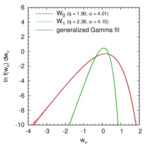
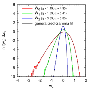
Figure 8: Distribution of scalar cell properties in a Poisson-Voronoi tessellation: The probability density is logarithmized, and its argument replaced by the reduced quantity $w_{\nu}:=\ln W_{\nu}-\mu(\ln W_{\nu})$. In this plot, a log-normal distribution would appear as a parabola with the apex on the $w=0$ line. The data is generated from $5\times 10^{7}$ (2D) and $10^{7}$ (3D) random Voronoi cells. Generalized Gamma distributions $\propto(W_{\nu})^{q(\alpha-1)}\exp(-(W_{\nu}/\theta)^{q})$ give good fits with the parameters specified in the plot key. ($\theta$ sets the length scale and is fixed by the normalization condition $\mu(w_{\nu})=0$.)

Table 2 shows results for the average scalar Minkowski functionals of Poisson-Voronoi cells. Analytical expressions are known for $W_{0}$ and $W_{1}$, and we find numerical values close to the exact results [15, 17]. The authors are not aware of an analytical expression for the average integral mean curvature $\mu(W_{2})$ of Poisson-Voronoi cells; the same is true for the standard deviations of the respective distributions. The scalar Minkowski functionals (area, perimeter in 2D and volume, surface area, integral mean curvature in 3D) are found to be compatible with generalized Gamma distributions in agreement with the literature (see fig. 8 in appendix and refs. [31, 17]).

	Fct.	$\mu(W_{\nu})$	exact $\mu(W_{\nu})$	$\sigma(W_{\nu})$
$D=2$	$W_{0}$	$1.00\rho^{-1}$	$\rho^{-1}$	$0.53\rho^{-1}$
	$W_{1}$	$2.00\rho^{-1/2}$	$2\rho^{-1/2}$	$0.49\rho^{-1/2}$
$D=3$	$W_{0}$	$1.00\rho^{-1}$	$\rho^{-1}$	$0.42\rho^{-1}$
	$W_{1}$	$1.94\rho^{-2/3}$	$\frac{4}{3}\smash{\left(\frac{4\pi}{3}\right)}^{1/3}\;\Gamma\!\left(\frac{5}{3}\right)\rho^{-2/3}$	$0.49\rho^{-2/3}$
	$W_{2}$	$3.05\rho^{-1/3}$	$-$	$0.78\rho^{-1/3}$

Table 2: Scalar Minkowski functionals of Voronoi cells induced by a Poisson point process. $\rho$ is the intensity of the point process, $\Gamma$ the Gamma function, and $D$ the spatial dimension. Exact results are taken from [17], numerical values estimated in the present study from 160,000 random Voronoi cells.

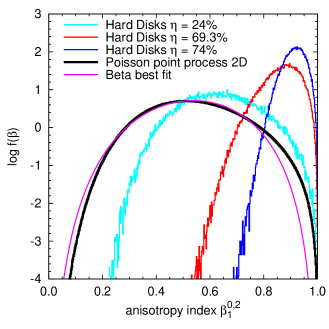
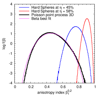
Figure 2: Distribution of the anisotropy index $\beta_{1}^{0,2}$ in configurations of hard disks (left) and spheres (right) of various packing fractions. The Poisson limit $\eta\rightarrow 0$ is indicated by the bold black line. Also shown is the best fit of a Beta distribution $\propto x^{m}(1-x)^{n}$ to the Poisson limit.

The mean and standard deviation of the distribution of the anisotropy indices $\beta_{\nu}^{a,b}$ of the Poisson-Voronoi cells are shown in table 3. Since the anisotropy indices are invariant under scaling, the length scale $\rho$ does not enter, and the tabulated values are fingerprints of a point pattern with uniformly and independently distributed germ points. The full distribution of $\beta_{1}^{0,2}$ values is shown in fig. 2 (bold lines). In the 3D case, it is approximately a Beta distribution, which is remarkable because the Beta distribution is closely related to the Gamma distribution. The agreement is less good in the 2D case.

	Tensor	$\mu(\beta_{\nu}^{a,b})$	$\sigma(\beta_{\nu}^{a,b})$
$D=2$	$W_{0}^{2,0}$	0.396	0.201
	$W_{1}^{2,0}$	0.463	0.197
	$W_{2}^{2,0}$	0.363	0.200
	$W_{1}^{0,2}$	0.540	0.180

	Tensor	$\mu(\beta_{\nu}^{a,b})$	$\sigma(\beta_{\nu}^{a,b})$
$D=3$	$W_{0}^{2,0}$	0.344	0.1330
	$W_{1}^{2,0}$	0.405	0.1330
	$W_{2}^{2,0}$	0.355	0.1301
	$W_{3}^{2,0}$	0.292	0.1261
	$W_{1}^{0,2}$	0.457	0.1251
	$W_{2}^{0,2}$	0.694	0.0871

Table 3: Mean and standard deviation of the anisotropy indices $\beta_{\nu}^{a,b}$ of the Voronoi cells induced by a Poisson point process. The intensity $\rho$ of the Poisson point process does not affect the dimensionless anisotropy indices.

4 Equilibrium Hard Spheres and Disks

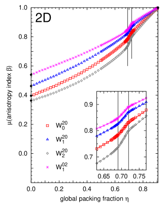
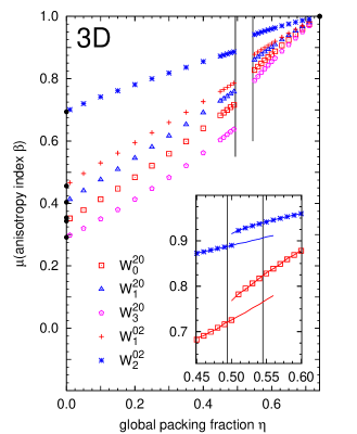
Figure 3: Average anisotropy indices $\beta$ for equilibrium ensembles of hard disks (left) and spheres (right) vs. packing fraction $\eta$. In the limit $\eta=0$, the hard spheres anisotropies are identical to those of the Poisson process (solid bullets). In 2D (left-hand side), changes of slope at the transition densities (magnified in inset) are observed. In 3D (right-hand side) the average $\beta$ displays a discontinuity at the first-order phase transition. The values of $\beta_{2}^{2,0}$ are very close to those of $\beta_{0}^{2,0}$ and have been omitted for the sake of clarity. The inset shows metastable states in or close to the coexistence region; symbols are Monte Carlo results, lines molecular dynamics simulations.

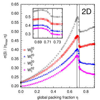
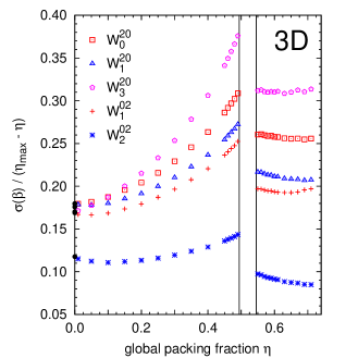
Figure 4: Standard deviations of the $\beta$ distribution for equilibrium hard disks (left) and spheres (right). A linear decrease as $\eta\rightarrow{\eta}_{\rm max}$ as been divided out. All data points calculated from Monte Carlo simulations. In the hard disks system, $\sigma(\beta)$ is continuous across the phase transition (magnified in inset). The hard spheres system show a discontinuity. The values of $\beta_{2}^{2,0}$ are very close to those of $\beta_{0}^{2,0}$ and have been omitted for the sake of clarity. Solid bullets on the plot frames represent the limit of the Poisson point process $\eta=0$.

The hard disks and hard spheres model is beyond doubt one of the most important generalizations of the ideal gas. This model, consisting in spherical particles without interaction other than elastic hard repulsion, possesses a fluid–solid phase transition [32, 33] and – in the 3D case – vitreous and jammed states [34]. In contrast to the ideal gas discussed above, the hard spheres model does have an intrinsic length scale by virtue of the particle radius and packing fraction $\eta$. This work focuses on monodisperse particles, even though the method is applicable to more general models when one replaces the Voronoi tessellation by a more general, for example the Apollonius tessellation [17].

Two different procedures have been employed to generate realizations of hard disks and hard spheres configurations: First, Monte Carlo (MC) simulations using alternating local Metropolis moves of single particles and collective cluster moves, specifically swaps of clusters between the configuration and its inversion at a randomly chosen point [35, 36]. Second, a 2D and a 3D event-driven molecular dynamics (MD) code solving Newton’s equations for a set of particles interacting via a hard spheres potential [37, 38]. All simulations are performed in the NV ensemble with periodic boundary conditions; particle numbers are 16,000 in the MC simulations (4,000 for the larger densities $\eta>0.6$ in 3D), and up to 256,000 in the MD 3D simulations. The starting configuration is an ordered triangular or fcc lattice.

The pair correlation functions of the resulting configurations are found to be in agreement with the Percus-Yevick approximation in the fluid phase [39]. The mean square displacement of the particles between two sampled configurations in the fluid phase is as large as the expectation for completely independent configurations, indicating a sufficiently equilibrated system. Away from the phase transition densities, both in 2D and 3D, the pair correlation functions from MC and MD are in agreement.

4.1 Averages of Anisotropy Indices

In similar fashion as with the Poisson data, a periodic Voronoi tessellation is computed for each configuration of particles, and Minkowski tensors and anisotropy indices are assigned to each particle. Fig. 3 shows the averages of $\beta_{\nu}^{a,b}$ for hard disks and hard spheres ensembles as a function of density. It is seen that increased order corresponds to more isotropic Voronoi cells in both hard disks and hard spheres.

We find MD and MC results to be in close agreement with each other except for in the vicinity of the hard spheres coexistence region. There, naturally, metastable states persist due to finite system sizes and simulation times, and the state of the system depends heavily on its history. The metastable fluid branch can be traced even beyond the fluid/solid coexistence region by choosing random initial conditions [40] instead of the usual fcc initial conditions (see fig. 3, inset in righthand side). Given enough simulation time, it would eventually form fcc nuclei and crystallize. The metastable fluid branch is distinctly more anisotropic on a local scale than the solid phase, again confirming the rule of thumb that more ordered systems are more locally isotropic.

In both MC and MD simulations, a discontinuity in the average anisotropy index $\mu(\beta_{\nu}^{a,b})$ is observed at the hard spheres phase transition, with the solid phase being more isotropic locally. At the same time, the standard deviation of the distribution of $\beta_{\nu}^{a,b}$ drops discontinuously across the transition; in the solid phase, it goes to zero almost linearly, $\sigma(\beta_{\nu}^{a,b})\propto(\eta-{\eta}_{\rm max})$, where ${\eta}_{\rm max}$ is the maximum global packing fraction.

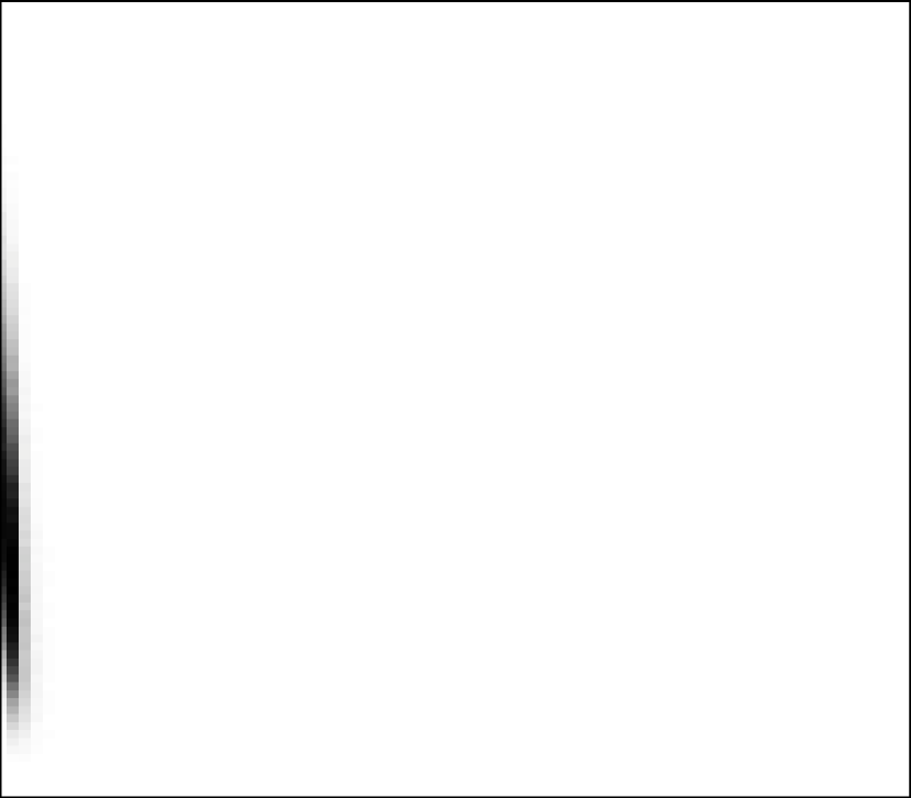
$\eta=0.01$

$\eta=0.05$

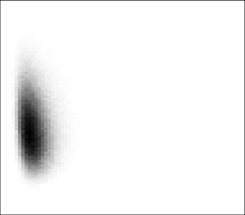
$\eta=0.10$

$\eta=0.15$

$\eta=0.20$

$\eta=0.25$

$\eta=0.30$

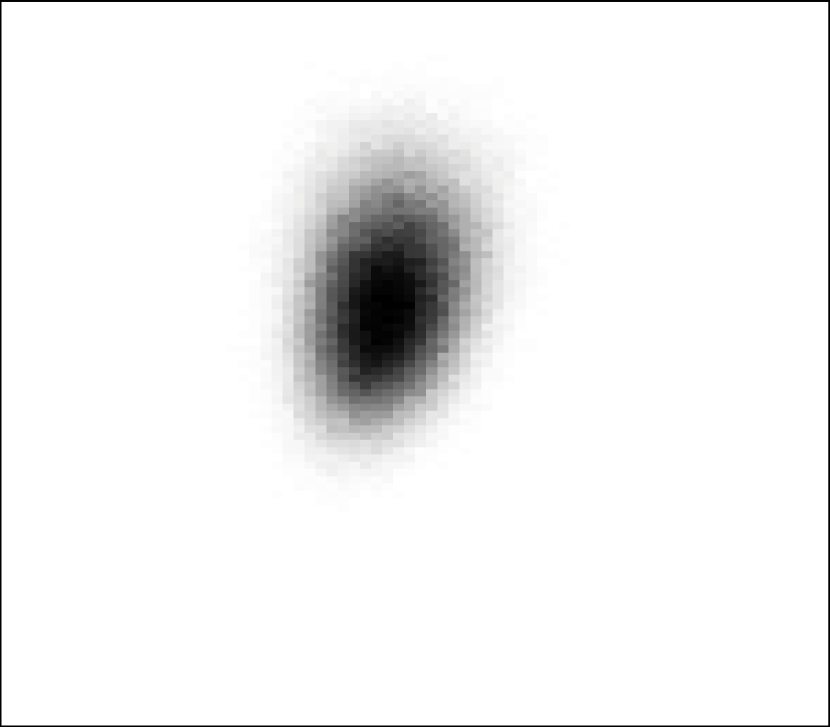
$\eta=0.35$

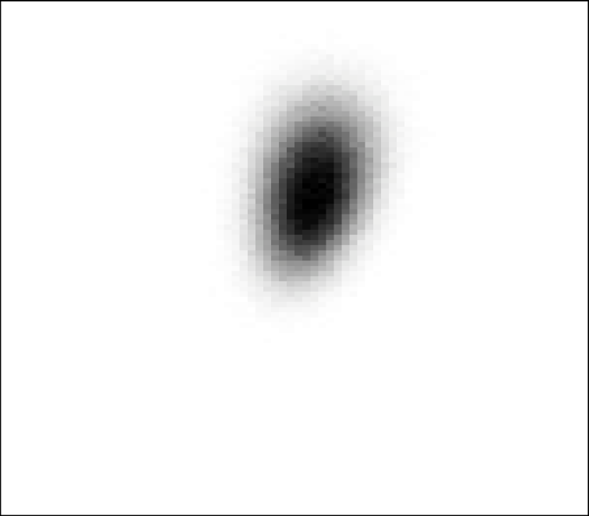
$\eta=0.40$

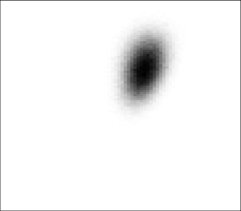
$\eta=0.45$

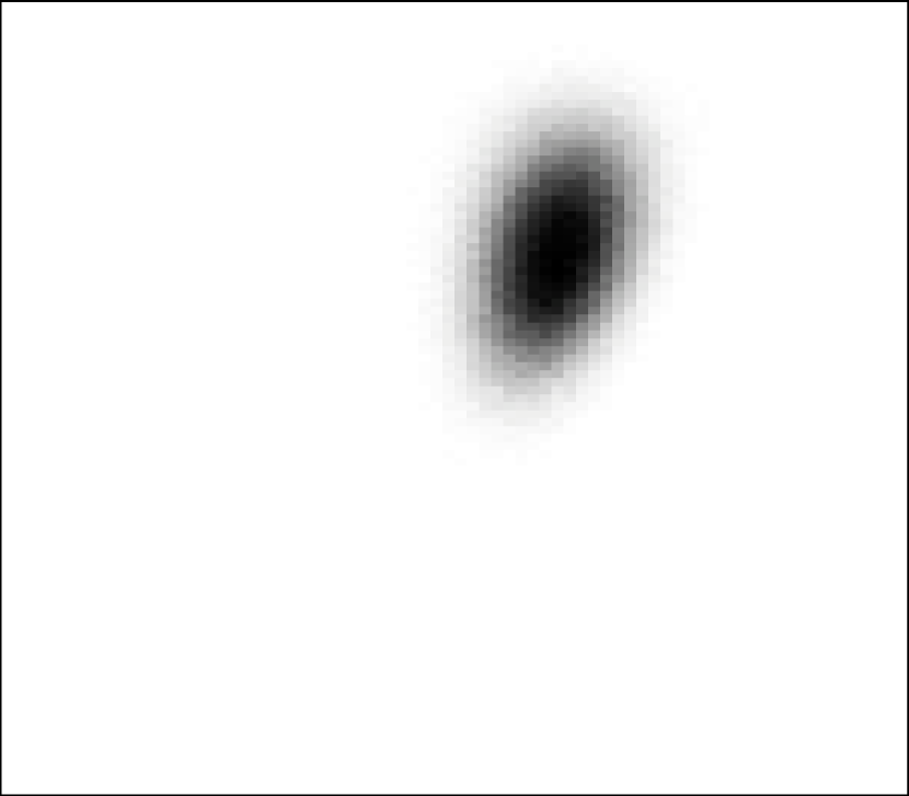
$\eta=0.46$

$\eta=0.47$

$\eta=0.48$

$\eta=0.49$

$\eta=0.50$

$\eta=0.51$

$\eta=0.52$

$\eta=0.53$

$\eta=0.54$

$\eta=0.55$

$\eta=0.56$

$\eta=0.57$

$\eta=0.58$

$\eta=0.59$

$\eta=0.60$

$\eta=0.61$

$\eta=0.63$

$\eta=0.65$

$\eta=0.67$

$\eta=0.71$

Figure 9: Histograms of anisotropy index $\beta_{0}^{2,0}$ and packing fraction $\eta$ of Voronoi cells in the hard spheres ensemble. The $x$ axis of each box shows the packing fraction $\eta^{(i)}\in[0;0.75]$ of individual cells, the $y$ axis shows the anisotropy parameter $\beta_{0}^{2,0}(K^{(i)})\in[0;1]$. Darker gray corresponds to larger probablity. The distribution changes characteristically from a triangular shape ($\eta<0.2$) to a ellipsoidal distribution for higher densities. In the limit $\eta\rightarrow\pi/\sqrt{18}\approx 0.74$, the distribution becomes a Dirac distribution $f(\eta,\beta)=\delta(\eta-\pi/\sqrt{18})\delta(1-\beta)$.

For large packing fractions, the system approaches the fcc state with isotropic cells only ($\mu=1$, $\sigma=0$). For small packing fractions, the Poisson limit is recovered, and $\mu$, $\sigma$ attain their respective values for the Poisson point process (bullets on the plot frame in figs. 3, 4). Remarkably, tensors $W_{2}^{2,0}$ and $W_{0}^{2,0}$ yield very similar anisotropy indices. No explanation for this data collapse has been identified. The shape of the distribution of $\beta$ values, seen in fig. 2, remains qualitatively similar and unimodal from the Poisson limit $\eta=0$ to the close-packed limit; its average value has a discontinuity at the phase transition. The development of the distribution function with varying packing fraction can be seen in fig. 9 in the appendix.

The situation in the hard disks system is less clear, and the nature of the phase transition has been the subject of continuous debate; current opinion favors a two-step transition according to the Kosterlitz-Thouless-Halperin-Nelson-Young scenario as opposed to a very weak transition of first order (see [41] and refs. therein).

Mean anisotropy indices show a change of slope at the transition densities (fig. 3, left-hand). In the transition region, we use systems of 64.000 disks in a hexagonal simulation cell with periodic boundary conditions. Wo find no significant differences between systems of 16.000 and 64.000 disks, given enough relaxation time. The $\mu(\beta)$ curves in fig. 3, left-hand side, and second moments $\mu(\beta^{2})$ behave linearly as prescribed by the lever rule, with coexistence densities of $\approx$0.70 and 0.72. Binder et al. [41] report closer values of 0.706 and 0.718. Full equilibration of the hard disks system in the transition region, however, remains difficult even with more advanced algorithms than the ones used in the present study [42].

4.2 Correlations among Anisotropy Indices

We find that the four (in 2D; six in 3D) different anisotropy indices display a qualitatively similar behavior. This shows that the anisotropy of the Voronoi cells is a generic feature and does not depend on the particular aspect of anisotropy being analyzed. Shapes can easily be constructed where the different Minkowski tensors yield widely different anisotropy indices. However, such shapes do not generally occur in a Voronoi tessellation.

This motivates the use of a single anisotropy index instead of the full set of Minkowski tensors. To justify this, we calculate the correlation coefficients ${\mathrm{corr}}(X,Y):={\mathrm{cov}}(X,Y)/(\sigma(X)\sigma(Y))$, ${\mathrm{cov}}(X,Y):=\mu((X-\mu(X))(Y-\mu(Y)))$, of the anisotropy indices; most pairings of $\beta_{\nu}^{a,b}$ are correlated with ${\mathrm{corr}}>0.8$ over the whole packing fraction range of the hard spheres ensemble. Only ${\mathrm{corr}}(\beta_{0}^{2,0},\beta_{2}^{0,2})$ gets as low as $0.7$ for the smallest packing fractions. The same is true for the hard disks ensemble, ${\mathrm{corr}}>0.8$ for most pairings; only ${\mathrm{corr}}(\beta_{0}^{2,0},\beta_{1}^{0,2})$ gets as low as 0.65 for the most dilute systems. It is thus justified, for the anisotropy analysis of the hard spheres ensemble, to focus on a single convenient anisotropy index, for example the translation invariant $\beta_{1}^{0,2}$. In the remainder of the article, we drop the indices $\nu,a,b$ off the $\beta$.

4.3 Comparison to Isoperimetric Ratio

Measures of asphericity have been previously used, e. g. the isoperimetric ratio (also called shape factor [9, 10]), defined by $\zeta:=(W_{1})^{2}(W_{0})^{-1}/\omega_{2}$ in two dimensions, and $\zeta:=(W_{1})^{3}(W_{0})^{-2}/\omega_{3}$ in three dimensions, with the volume $\omega_{D}$ of the $D$-dimensional unit sphere. Starr et al. use an asphericity index based on closest neighbors distance in the Voronoi tessellation [11].

The distinction between asphericity, meaning deviations of the shape from a sphere, and anisotropy, meaning that the object has different spatial extension or surface area in different spatial directions, is subtle. Clearly, a sphere’s isoperimetric ratio can be increased by applying an undulation to the bounding surface or by deforming it into a cube. Both leave the anisotropy unchanged. On the other hand, $\zeta$ also changes when the sphere is deformed into an ellipsoid, becoming anisotropic. The anisotropy indices $\beta$ clearly distinguish between asphericity and anisotropy. Also, the Minkowski tensors not only provide a convenient anisotropy index, but also identify explicitly, by means of the eigenvectors, the preferred directions for each cell. Accordingly, we find that $\zeta$ is less correlated with the $\beta$ indices than the set of $\beta$ among themselves; ${\mathrm{corr}}(\zeta,\beta_{\nu}^{a,b})$ ranges between $-0.6$ and $-0.2$ for all $\beta_{\nu}^{a,b}$ both in two and three dimensions, meaning that the Minkowski tensors probe a different aspect of the cell shapes than the isoperimetric ratio alone.

It is noteworthy that the isoperimetric ratio follows a double-peak distribution in the hard disks system [9]. The distribution of the $\beta$ indices, however, is unimodal, see fig. 2; it changes continuously across the solid/fluid phase transition.

5 Lennard-Jones fluid

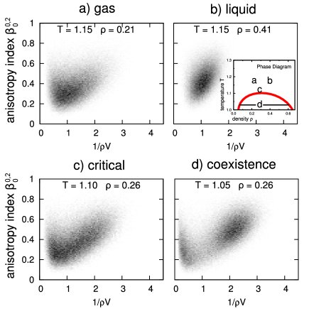
Figure 5: Histograms of the Voronoi cell anisotropy and density at four points in the Lennard-Jones phase diagram (sketched in inset): a) vapor state b) liquid state c) critical composition d) coexistence of liquid and vapor. The systems consist of 100.000 particles each. The $x$ axis shows a local normalized density given by the reciprocal cell volume $V$ in units of the global density $\rho$, while the $y$ axis shows the anisotropy index $\beta_{0}^{2,0}$. A more complete survey of the phase diagram is found in the appendix (fig. 10).

Configurations of Lennard-Jones (LJ) fluids with 100.000 particles in periodic boundary conditions are generated using a parallel molecular dynamics code [43, 44]. The LJ fluid is a true thermal system, the phase diagram is two-dimensional, and includes a critical point. The precise location of the critical point depends on the numerical treatment of the LJ potential, in particular the cutoff radius and cutoff corrections [45]. Here, a cutoff of $2.5r_{0}$ is chosen.

For the pointlike LJ particles, we consider, as previously in fig. 1, the local normalized (particle number) density $d^{(i)}=1/(\rho V^{(i)})$, where $\rho$ is the global particle number density, and the volume $V^{(i)}:=W_{0}(K^{(i)}{})$ is the volume of Voronoi cell $K^{(i)}{}$. Thus, $\mu\bigl{(}1/d^{(i)}\bigr{)}=1$. Fig. 5 shows two-parameter histograms of the densities $d^{(i)}$ and anisotropy indices $\beta_{0}^{2,0}(K^{(i)}{})$ of Voronoi cells in LJ configurations. Configurations from four points in the LJ phase diagram are shown, and the corresponding locations indicated in the phase diagram sketch (inset). In the high-temperature limit, above the critical point, we find a continuous change of the probablity distribution from a triangular shape (subfigure a) as is also found for the ideal gas (fig. 1) to a ellipsoidal shape (subfigure b) as is found in the hard spheres system (also seen in fig. 1). Below the critical point, coexisting liquid and vapor phases can be clearly distinguished as two components of the probability distribution (subfigure d). These components grow closer as the temperature is increased, and eventually merge at the critical point (subfigure c).

6 Robustness of the Minkowski Tensors

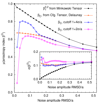
Figure 6: Left: Anisotropy index for $W_{1}^{0,2}(K^{(i)}{})$ and Edwards’ configurational tensor $C^{(i)}$, applied to a fcc Einstein solid. The noise amplitude is quantified by the root mean square displacement ${\mathrm{RMSD}}$ of the germs from their ideal lattice sites. The Minkowski tensor $W_{1}^{0,2}(K^{(i)}{})$ is computed from the Voronoi tessellation of the lattice, $C^{(i)}$ is computed with the Delaunay neighborhood and distance cutoff neighborhoods of the order of the noise amplitude. It is seen that, even for vanishingly small levels of noise, $C^{(i)}$ of a single lattice site is not an isotropic tensor, while $W_{1}^{0,2}(K^{(i)}{})$ is. Tensor isotropy is defined via the ratio of eigenvalues, as in eq. (6). The $x$ axis and cutoffs are in units of the fcc nearest neighbor distance $a$. Right: Illustration of point configuration with a degenerate Delaunay triangulation. A small perturbation (not drawn to scale) lifts the degeneracy and breaks the isotropic 4-simplices into anisotropic triangles.

A simple model of a thermal solid is defined by putting the germs on an ideal lattice, and allowing each germ to deviate by a small distance $\vec{\varepsilon}^{\;(i)}$ from its ideal site, as in the Einstein solid. We generated a point configuration by drawing, independently for each lattice site, the random displacement vector $\vec{\varepsilon}^{\;(i)}$ from a three-dimensional Gaussian distribution. The set of germs is then $\{\vec{g}^{\;(i)}=\vec{l}^{\;(i)}+\vec{\varepsilon}^{\;(i)}\}$, where $l^{(i)}$ are the fcc lattice sites. The noise amplitude is given by the root mean square displacement (RMSD) of the particles, ${\mathrm{RMSD}}=\sqrt{\mu(|\vec{\varepsilon}^{\;(i)}|^{2})}$; since the expectation value of $\vec{\varepsilon}^{\;(i)}$ vanishes, ${\mathrm{RMSD}}=\sigma(\vec{\varepsilon}^{\;(i)})$. Increasing the noise amplitude eventually destroys lattice order und yields a Poisson point pattern. This model neglects correlations between displacements of different particles that necessarily exist in a real solid, and does allow for overlap if the particles have finite radius.

In fig. 6, as the noise amplitude is increased, $\mu(\beta_{1}^{0,2})$ decreases continuously from unity, similarly as it does when decreasing packing fraction $\eta$ from the maximum density state in the hard spheres model (fig. 3). In the limit of strong noise, the anisotropy index of the Poisson point pattern is recovered ($\mu(\beta_{1}^{0,2})\rightarrow 0.457$).

6.1 Robustness against Noise

The Minkowski tensors of Voronoi cells vary continuously when germs as dislocated. The topology of the Voronoi tessellation may change; however, the shape of the Voronoi cells $K^{(i)}$ is a continuous function of the germ point locations. For example, it is possible that a small dislocation of a germ creates additional facets in the Voronoi tessellation; however, since these new faces are very small, and their contribution to the tensor of the cell is weighted with their area, only a small change in the tensor is effected.

This continuity property is not necessarily guaranteed for other, similarly defined shape measures. For example, Edwards et al. [12, 46] defined a configurational tensor

$${C^{(i)}}:=\sum_{j\in{\mathrm{NN}}(i)}(\vec{r}^{\,(i)}-\vec{r}^{\,(j)})\otimes(\vec{r}^{\,(i)}-\vec{r}^{\,(j)})$$ (7)

with some suitable definition for the set NN of nearest neighbors. NN may be defined using the Delaunay triangulation, or a fixed cutoff radius, or physical contacts. If, under a small dislocation of a germ, the neighborhood NN changes, a comparatively large change of the tensor results, because the bond vector $\vec{r}^{\;(i)}-\vec{r}^{\;(j)}$ to the lost or newly gained neighbor tends to be larger than the other bond vectors. Consequently, $C^{(i)}$ changes discontinuously.

The discontinuous behavior of $C^{(i)}$ is especially pronounced for near-degenerate configurations, for example the fcc lattice with vanishingly small noise amplitude. As fig. 6 shows, $C^{(i)}$ is not an isotropic tensor at zero noise, even though a fcc lattice site has 12 symmetrically arranged nearest neighbors. This is due to numerical roundoff errors. For simplicity, we discuss the two-dimensional case, which exhibits the same conceptual problem. Consider the perfect square lattice in fig. 6. The Delaunay simplices are not, as in a general point pattern, triangles, but degenerate to squares. $C^{(i)}$ computed from such simplices is an isotropic tensor. However, tiny amounts of numerical inaccuracy or noise lift the degeneracy for some of the squares and cause the squares to break up into triangles [29]. $C^{(i)}$ computed from the triangles is no longer an isotropic tensor. Due to the same effect in three dimensions, $C^{(i)}$ with the Delaunay neighborhood is not a good measure of anisotropy.

Note that the Minkowski tensor $W_{1}^{0,2}$ is similar to the Edwards tensor as the normal directions of Voronoi facets are precisely the directions of the bond vectors via the Voronoi–Delaunay duality. However, the weighting with the facet area in eq. (5) ensures that the tensor is a continuous function of the germ point locations.

6.2 Discrimination of Einstein Solid and Hard Spheres Equilibrium Solid

As shown above, the mean anisotropy index $\mu(\beta)$ of the Einstein solid decreases with increasing noise amplitude, similar to the hard spheres solid. However, the two point patterns are clearly structurally different, as the hard spheres system includes correlations between individual particles.

To see this, it is again useful to study the correlation between local normalized density $d$ and local anisotropy $\beta$. Figure 7 shows that $d^{(i)}$ is negatively correlated with $\beta(K^{(i)}{})$ for the Einstein solid (blue dashed line), while the two variables are positively correlated for the hard spheres solid (red solid line). Positive correlation is the rule for interacting systems such as hard spheres, and has also been found for jammed bead packs [4], while a negative correlation has been found for foam models.

This can be understood considering that, for the hard spheres solid, a higher density implies that the cell shape is closer to the shape of the particle since particles cannot overlap. On the other hand, for the Einstein solid, no minimum distance is enforced, and high densities are the result of one germ intruding into the domain of another, creating two oblate Voronoi cells.

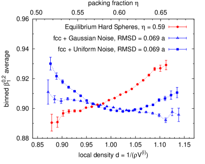
Figure 7: Comparison of average anisotropy index $\beta_{1}^{0,2}$ as a function of local normalized densities $d$. The Voronoi cells are binned in density bins, and an average of their anisotropy indices is computed separately for each bin. The error bars are estimated from standard deviations in each bin. The plot shows that the correlation of anisotropy index and cell volume distinguishes between the Einstein solid and the equilibrium hard spheres structure (in the solid phase), even though parameters were chose such that the global averages $\mu(\beta_{1}^{0,2})$ are equal.

Conclusions

This study shows how Minkowski tensors can be used to characterize point patterns, and in particular their local anisotropy. A simple, linear algorithm to compute the shape tensors of a polyhedron was given elsewhere [25, 26].

Particle configurations from a number of fluid models are analyzed using the Minkowski tensor framework, and reference values for these idealized systems are given. In each of the systems, the Minkowski tensor analysis is able to quantify the morphological properties of the system in a robust way. The continuity properties guarantee that small shifts in the germ positions do not influence the result in an undue manner, as is the case for a naïvely defined “bond tensor”. In particular, $W_{1}^{0,2}$ is found to include the correct weighting prefactors of the bond vectors to ensure continuity.

The anisotropy analysis is found to be sensitive to the phase behavior of the fluids, and the average anisotropy index may be used to distinguish collective states of the fluid. More research is needed in order to link order parameters based on Minkowski tensors with more established order parameters like the bond-angle [5] order parameter. For the hard spheres system, exact relations between the equations of state and the geometry of the available space, in particular its surface area and volume, are known to exist [47, 48, 49, 50]. Similar relations are not yet known for Minkowski tensors of available space. However, a density functional theory based on Minkowski tensors of convex particles has been developed, and provides accurate approximations for the equations of state [51, 52, 53]. Finally, the application of the Minkowski tensors to a comprehensive set of experimental data is desirable. For the latter purpose, the Minkowski tensor software may be freely downloaded from the institute homepage at

http://www.theorie1.physik.uni-erlangen.de/

References

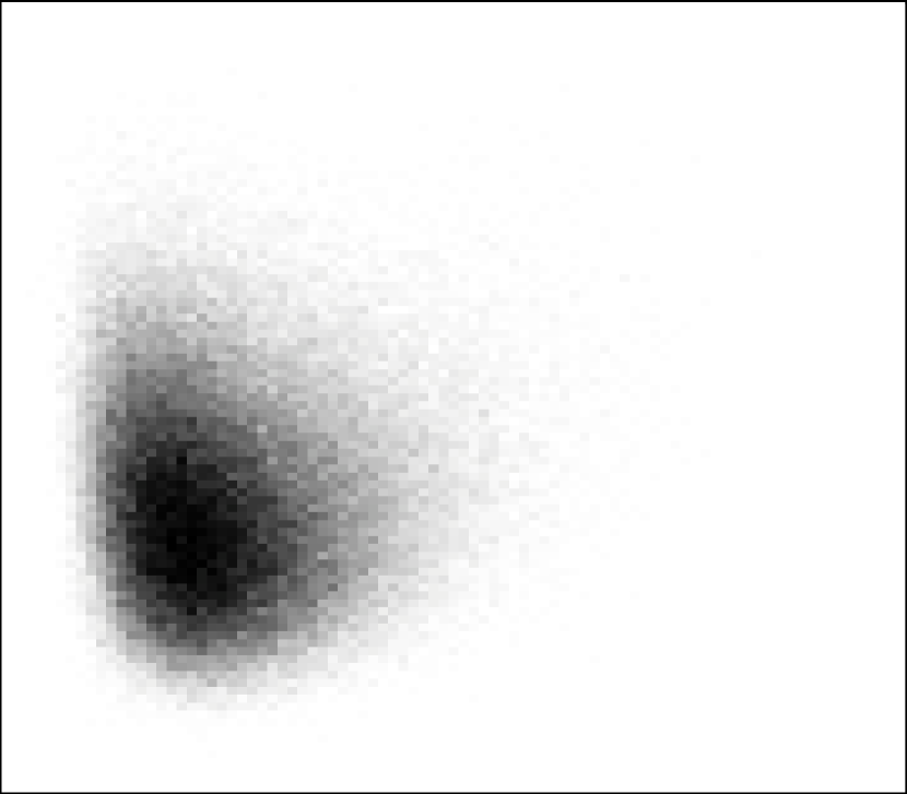
$T=1.50$

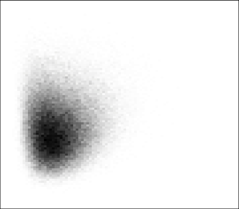
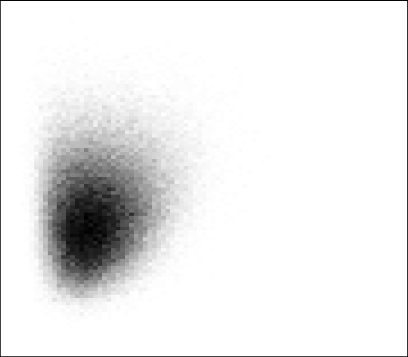
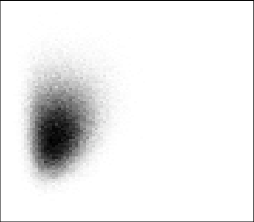
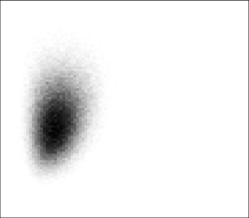
$T=1.15$

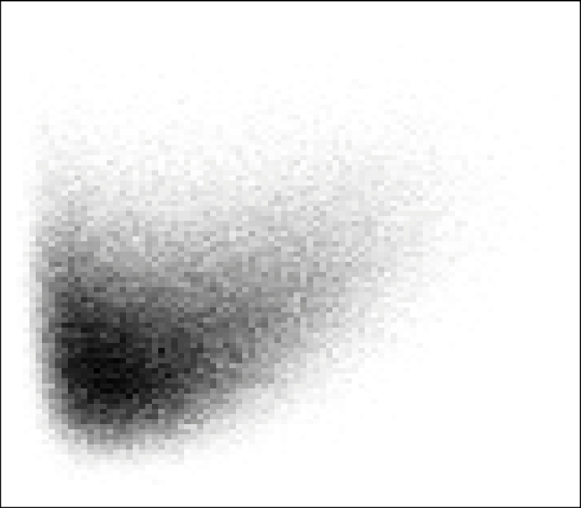
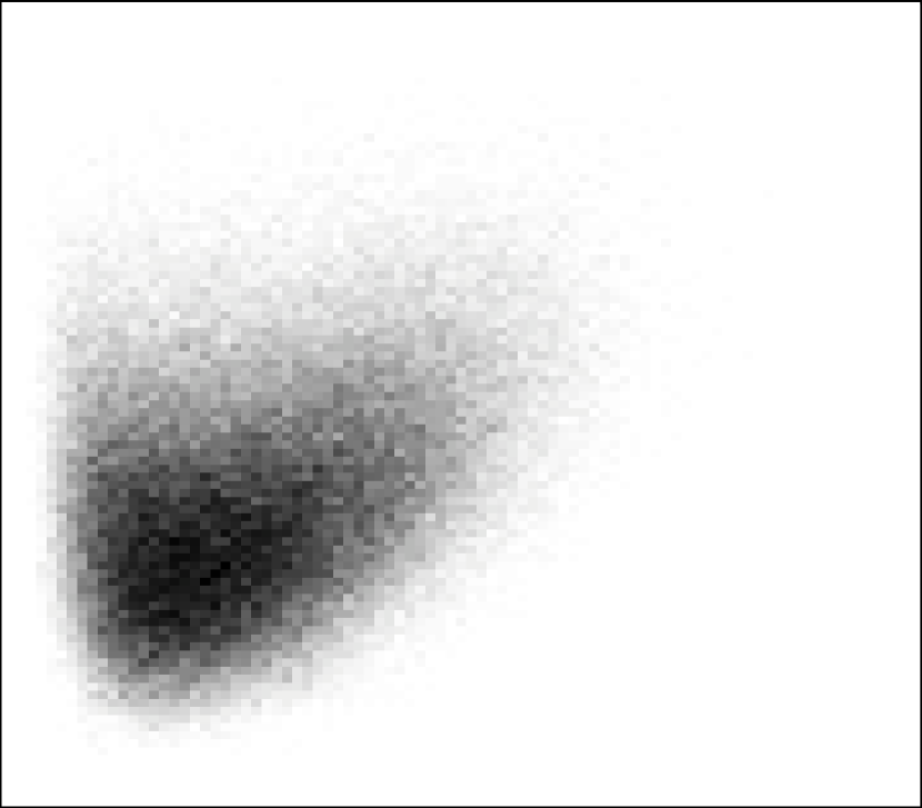
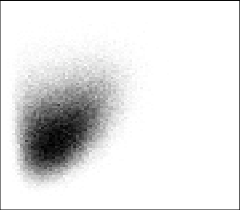
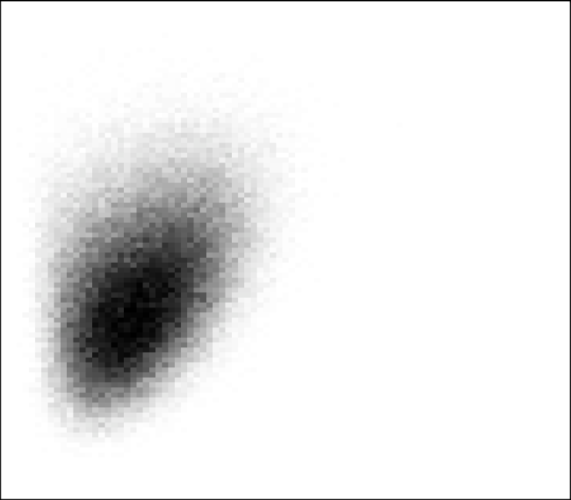
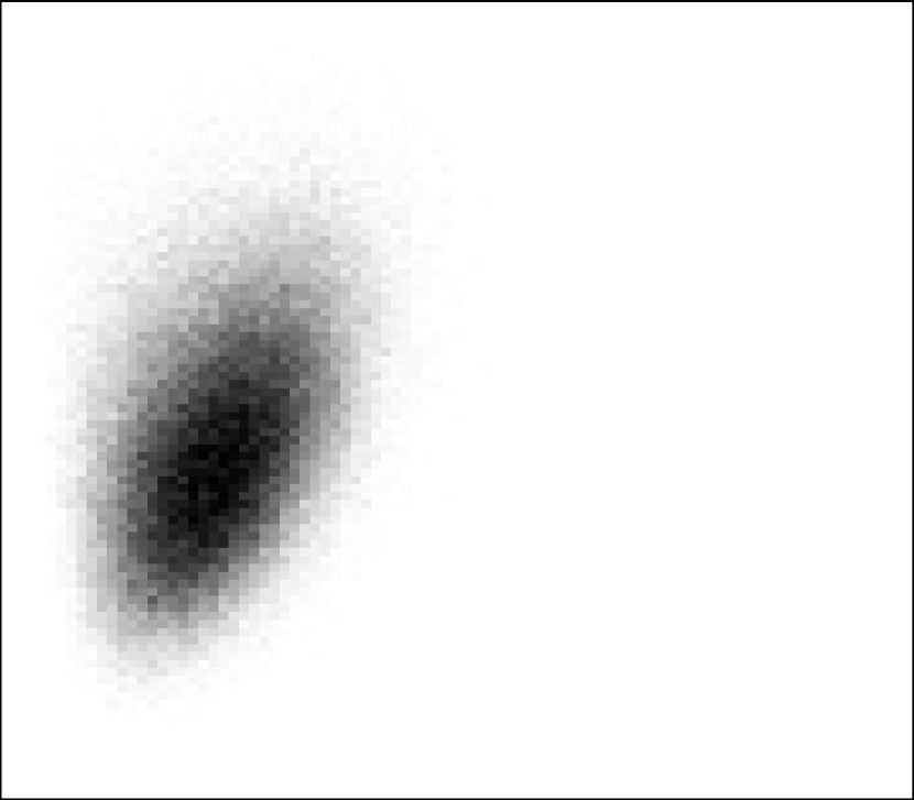
$T=1.10$

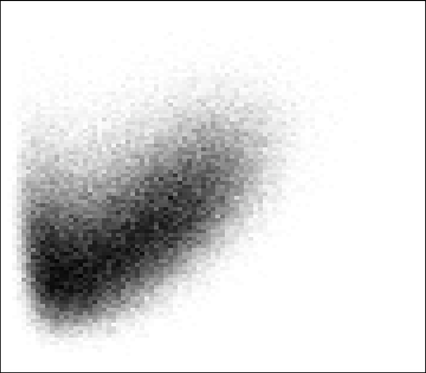
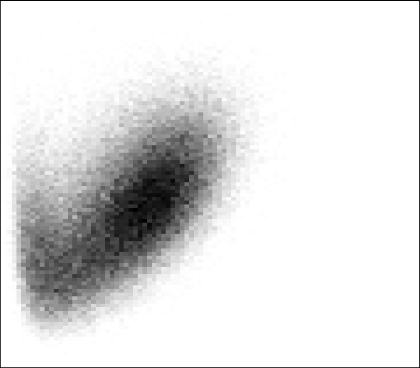
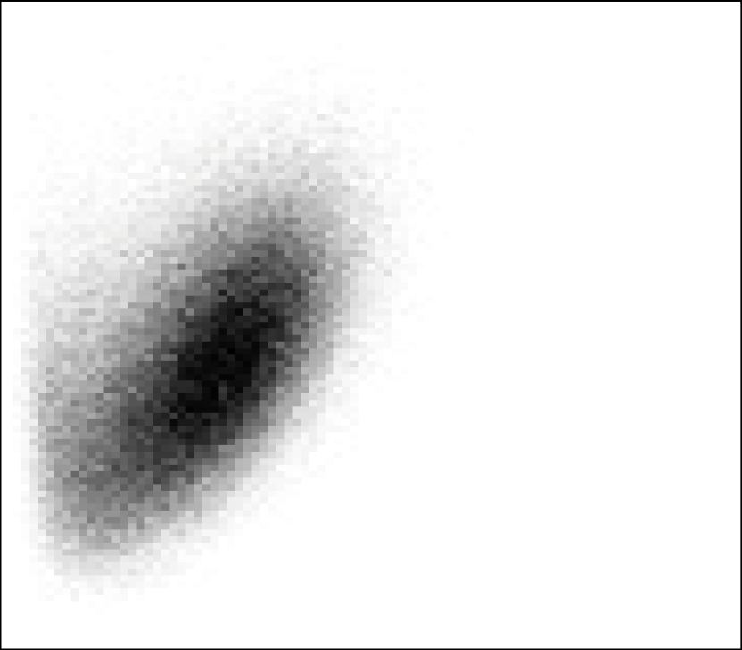
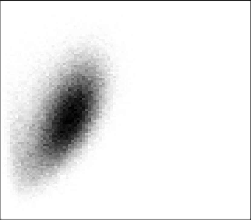
$T=1.05$

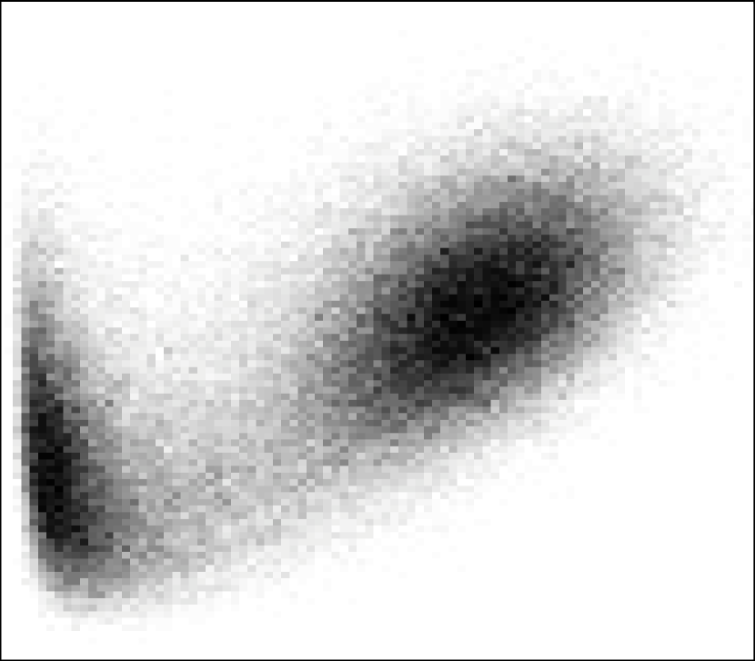
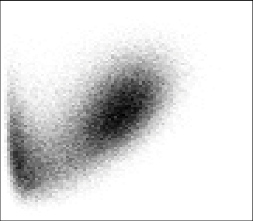
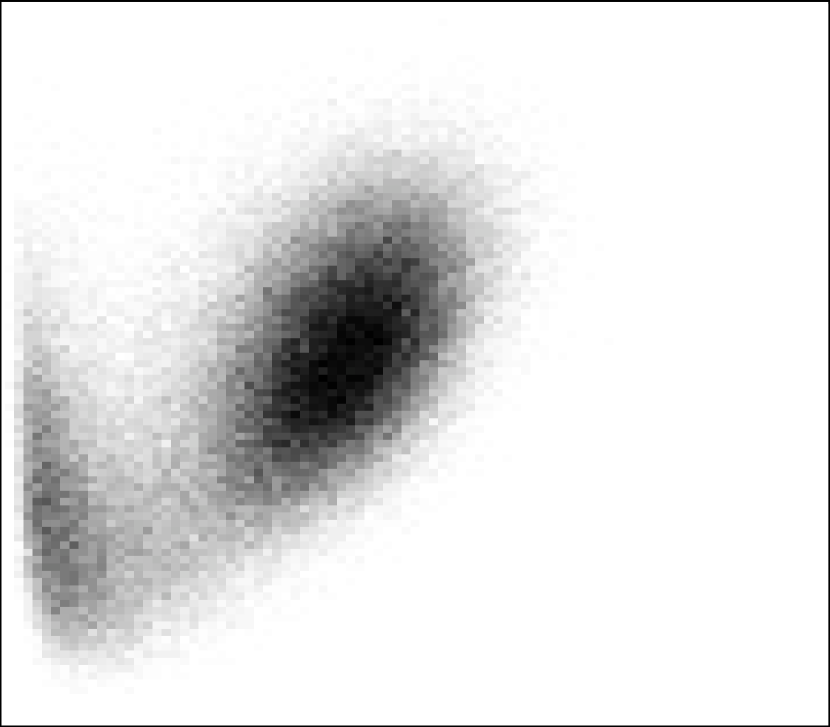
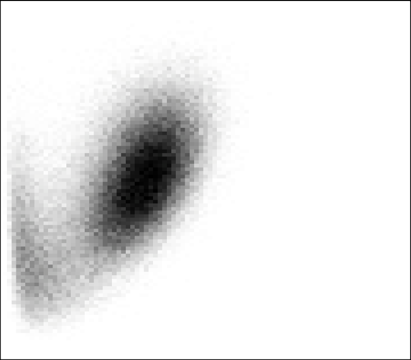
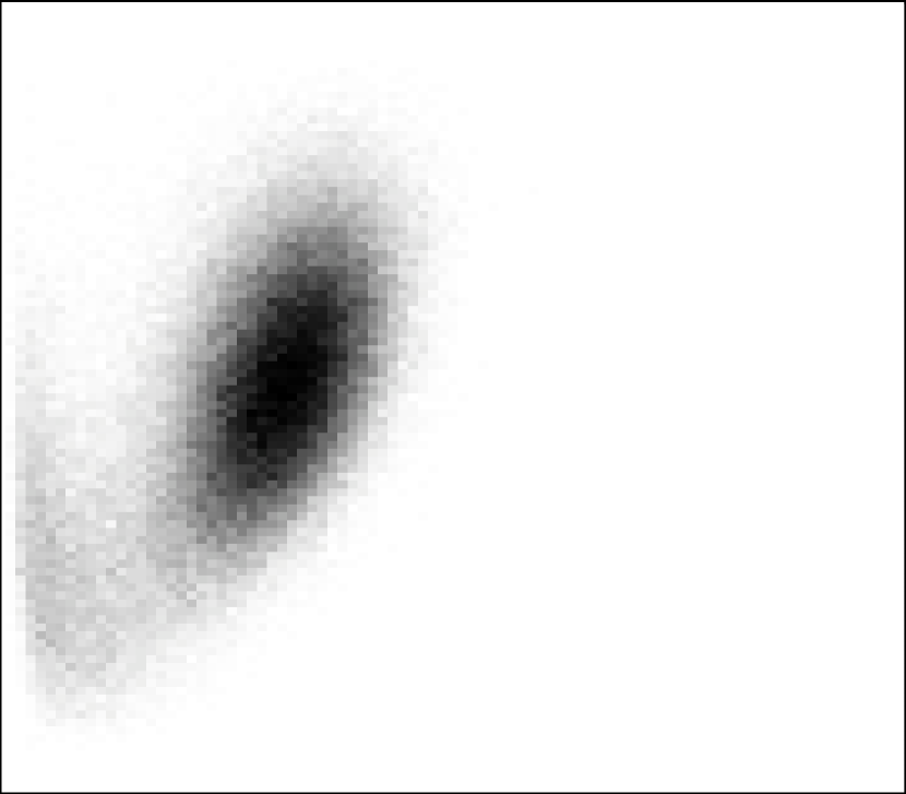
$\rho=0.21$

$\rho=0.26$

$\rho=0.31$

$\rho=0.36$

$\rho=0.41$

Figure 10: Histograms of $\beta_{0}^{2,0}$ and $d$ for Lennard-Jones configurations. The $x$ axis of each box shows local particle number density $d^{(i)}\in[0;4.5]$ of individual Voronoi cells, the $y$ axis shows the anisotropy parameter $\beta_{0}^{2,0}(K^{(i)})\in[0;1]$. The critical point would correspond to the configuration at $T=1.1$ and $\rho=0.26$; below, vapor/liquid coexistence is found; above, a single fluid phase exists and the probability distribution only has a single component.

References

- [1] Peter Wochner, Christian Gutt, Tina Autenrieth, Thomas Demmer, Volodymyr Bugaev, Alejandro Díaz Ortiz, Agnès Duri, Federico Zontone, Gerhard Grübel, and Helmut Dosch. X-ray cross correlation analysis uncovers hidden local symmetries in disordered matter. Proceedings of the National Academy of Sciences, 106(28):11511–11514, 2009.
- [2] H. Reichert, O. Klein, H. Dosch, M. Denk, V. Honkim ki, T. Lippmann, and G. Reiter. Observation of five-fold local symmetry in liquid lead. Nature, 408:839–841, 2000.
- [3] Eric R. Weeks, J. C. Crocker, Andrew C. Levitt, Andrew Schofield, and D. A. Weitz. Three-Dimensional Direct Imaging of Structural Relaxation Near the Colloidal Glass Transition. Science, 287(5453):627–631, 2000.
- [4] Gerd E. Schröder-Turk, Walter Mickel, Matthias Schröter, Gary W. Delaney, Mohammad Saadatfar, Tim J. Senden, Klaus Mecke, and Tomaso Aste. Disordered spherical bead packs are anisotropic. Europhysics Letters, 90:34001, 2010.
- [5] A. C. Mitus, H. Weber, and D. Marx. Local structure analysis of the hard-disk fluid near melting. Phys. Rev. E, 55(6):6855–6859, 1997.
- [6] Salvatore Torquato, Thomas M. Truskett, and Pablo G. Debenedetti. Is random close packing of spheres well defined? Phys. Rev. Lett., 84(10):2064–2067, Mar 2000.
- [7] Takeshi Kawasaki, Takeaki Araki, and Hajime Tanaka. Correlation between dynamic heterogeneity and medium-range order in two-dimensional glass-forming liquids. Phys. Rev. Lett., 99(21):215701, Nov 2007.
- [8] Wolfgang Lechner and Christoph Dellago. Accurate determination of crystal structures based on averaged local bond order parameters. Journal of Chemical Physics, 129:114707, 2008.
- [9] Filip Moučka and Ivo Nezbeda. Detection and characterization of structural changes in the hard-disk fluid under freezing and melting conditions. Phys. Rev. Lett., 94(4):040601, Feb 2005.
- [10] P. M. Reis, R. A. Ingale, and M. D. Shattuck. Crystallization of a quasi-two-dimensional granular fluid. Phys. Rev. Lett., 96(25):258001, Jun 2006.
- [11] Francis W. Starr, Srikanth Sastry, Jack F. Douglas, and Sharon C. Glotzer. What do we learn from the local geometry of glass-forming liquids? Phys. Rev. Lett., 89(12):125501, Aug 2002.
- [12] Sam F. Edwards and D. V. Grinev. Transmission of stress in granular materials as a problem of statistical mechanics. Physica A: Statistical Mechanics and its Applications, 302(1-4):162 – 186, 2001.
- [13] Raphael Blumenfeld and Sam F. Edwards. Granular entropy: Explicit calculations for planar assemblies. Phys. Rev. Lett., 90(11):114303, 2003.
- [14] G. Durand, F. Graner, and J. Weiss. Deformation of grain boundaries in polar ice. Europhys. Lett., 67:1038–1044, 2004.
- [15] J.L. Meijering. Interface area, edge length, and number of vertices in crystal aggregates with random nucleation. Research Report 8, Philips, 1953.
- [16] John D. Bernal. A geometrical approach to the structure of liquids. Nature, 183:141–147, 1959.
- [17] A. Okabe, B. Boots, K. Sugihara, and S. N. Chiu. Spatial tesselations: Concepts and applications of Voronoi diagrams. John Wiley, second edition, 2000.
- [18] D. Frenkel, B. M. Mulder, and J. P. McTague. Phase diagram of a system of hard ellipsoids. Phys. Rev. Lett., 52(4):287–290, Jan 1984.
- [19] J. A. C. Veerman and D. Frenkel. Phase diagram of a system of hard spherocylinders by computer simulation. Phys. Rev. A, 41(6):3237–3244, Mar 1990.
- [20] L. J. Ellison, D. J. Michel, F. Barmes, and D. J. Cleaver. Entropy-driven formation of the gyroid cubic phase. Phys. Rev. Lett., 97(23):237801, 2006.
- [21] Hugo Hadwiger. Vorlesungen über Inhalt, Oberfläche und Isoperimetrie. Springer, 1957.
- [22] Luís A. Santaló. Integral Geometry and Geometric Probability. Addison-Wesley, 1976.
- [23] Klaus Mecke. Additivity, convexity, and beyond: Applications of Minkowski functionals in statistical physics. In Klaus Mecke and Dietrich Stoyan, editors, Statistical Physics and Spatial Statistics – The Art of Analyzing and Modeling Spatial Structures and Patterns, volume 554 of Lecture Notes in Physics, pages 111–184. Springer Verlag, 2000.
- [24] S. Alesker. Description of continuous isometry covariant valuations on convex sets. Geom. Dedicata, 74:241–248, 1999.
- [25] Gerd E. Schröder-Turk, Sebastian C. Kapfer, Boris Breidenbach, Claus Beisbart, and Klaus Mecke. Tensorial Minkowski functionals and anisotropy measures for planar patterns. J. of Microscopy, 238:57–74, 2010.
- [26] Gerd E. Schröder-Turk, Walter Mickel, Sebastian C. Kapfer, Fabian M. Schaller, Daniel Hug, Boris Breidenbach, and Klaus Mecke. Minkowski Tensors of anisotropic spatial structure. in preparation, 2010.
- [27] D. Hug, R. Schneider, and R. Schuster. The space of isometry covariant tensor valuations. St. Petersburg Math. J., 19:137–158, 2008.
- [28] Tomaso Aste and Tiziana DiMatteo. Emergence of Gamma distributions in granular materials and packing models. Phys. Rev. E, 77:021309, 2008.
- [29] C.B. Barber, D.P. Dobkin, and H. Huhdanpaa. The Quickhull algorithm for convex hull. ACM Transactions on Mathematical Software, 22(4):469–483, 1996.
- [30] Rolf Schneider and Wolfgang Weil. Stochastic and Integral Geometry (Probability and Its Applications). Springer, 2008.
- [31] Howard G. Hanson. Voronoi cell properties from simulated and real random spheres and points. Journal of Statistical Physics, 30(3):591–605, 1983.
- [32] B. J. Alder and T. E. Wainwright. Phase transition for a hard sphere system. The Journal of Chemical Physics, 27(5):1208–1209, 1957.
- [33] W. W. Wood and J. D. Jacobson. Preliminary results from a recalculation of the monte carlo equation of state of hard spheres. The Journal of Chemical Physics, 27(5):1207–1208, 1957.
- [34] S. R. Williams, I. K. Snook, and W. van Megen. Molecular dynamics study of the stability of the hard sphere glass. Phys. Rev. E, 64(2):021506, Jul 2001.
- [35] Werner Krauth. Statistical Mechanics: Algorithms and Computations. Oxford University Press, 2006.
- [36] Christophe Dress and Werner Krauth. Cluster algorithm for hard spheres and related systems. Journal of Physics A: Mathematical and General, 28:L597–L601, 1995.
- [37] D.C. Rapaport. The Art of Molecular Dynamics Simulation. (Cambridge University Press, 2 edition, 2004.
- [38] Masaharu Isobe. Simple and efficient algorithm for large-scale molecular dynamics simulation in hard-disk system. International Journal of Modern Physics C, 10:1281–1293, 1999.
- [39] Vitaly I. Kalikmanov. Statistical Physics of Fluids. Springer, 2001.
- [40] Shigenori Matsumoto, Tomoaki Nogawa, Takashi Shimada, and Nobuyasu Ito. Heat transport in a random packing of hard spheres, 2010. arXiv:1005.4295v1 [cond-mat.stat-mech].
- [41] Kurt Binder, Surajit Sengupta, and Peter Nielaba. The liquid-solid transition of hard discs: first-order transition or Kosterlitz-Thouless-Halperin-Nelson-Young scenario? Journal of Physics: Condensed Matter, 14(9):2323, 2002.
- [42] Etienne P. Bernard, Werner Krauth, and David B. Wilson. Event-chain monte carlo algorithms for hard-sphere systems. Phys. Rev. E, 80(5):056704, Nov 2009.
- [43] Christian Goll. Algorithms for molecular dynamics simulations in fluids. PhD thesis, Friedrich-Alexander Universität Erlangen-Nürnberg, 2010.
- [44] Daan Frenkel and Berend Smit. Understanding Molecular Simulation. Academic Press, 2 edition.
- [45] Andrij Trokhymchuk and José Alejandre. Computer simulations of liquid/vapor interface in Lennard-Jones fluids: Some questions and answers. The Journal of Chemical Physics, 111(18):8510–8523, 1999.
- [46] Hernan A. Makse, Jasna Brujic, and Sam F. Edwards. Statistical mechanics of jammed matter. In Haye Hinrichsen and Dietrich E. Wolf, editors, The Physics of Granular Media, pages 45–86. Wiley-VCH, 2004.
- [47] Robin J. Speedy. Statistical geometry of hard-sphere systems. J. Chem. Soc. Faraday Trans. II, 76:693–703, 1980.
- [48] Robin J. Speedy and Howard Reiss. Cavities in the hard sphere fluid and crystal and the equation of state. Molecular Physics, 72:999–1014, 1991.
- [49] David S. Corti and Richard K. Bowles. Statistical geometry of hard sphere systems: exact relations for additive and non-additive mixtures. Molecular Physics, 96:1623–1635, 1999.
- [50] Srikanth Sastry, Thomas M. Truskett, Pablo G. Debenedetti, Salvatore Torquato, and Frank H. Stillinger. Free volume in the hard sphere liquid. Molecular Physics, 95:289–297, 1998.
- [51] Yaakov Rosenfeld. Free-energy model for the inhomogeneous hard-sphere fluid mixture and density-functional theory of freezing. Phys. Rev. Lett., 63:980, 1989.
- [52] Hendrik Hansen-Goos and Klaus Mecke. Fundamental measure theory for inhomogeneous fluids of non-spherical hard particles. Phys. Rev. Letters, 102:018302, 2009.
- [53] Hendrik Hansen-Goos and Klaus Mecke. Tensorial density functional theory for non-spherical hard-body fluids. J. Phys.: Condens. Matter, 22:364107, 2010.